Generalizing the Orbifold Model for Voice Leading

Abstract

We generalize orbifold models for chords and voice leading to incorporate loudness, allowing for the modeling of resting voices, which are used frequently by composers and arrangers across genres. In our generalized setting (strictly speaking, that of orbispaces rather than an orbifolds), passages with resting voices, passages with two or more voices in unison, and fully harmonized passages occupy distinct subspaces that interact in mathematically precise and musically interesting ways. In particular, our setting includes previous orbifold models by way of constant-loudness subspaces, and provides a way to model voice leading between chords of different cardinalities. We model voice leading in this general setting by morphisms in the orbispace path groupoid, a category for which we give a formal definition. We demonstrate how to visualize such morphisms as singular braids, and explore how our approach relates to (and is consistent with) selected previous work.

1. Introduction

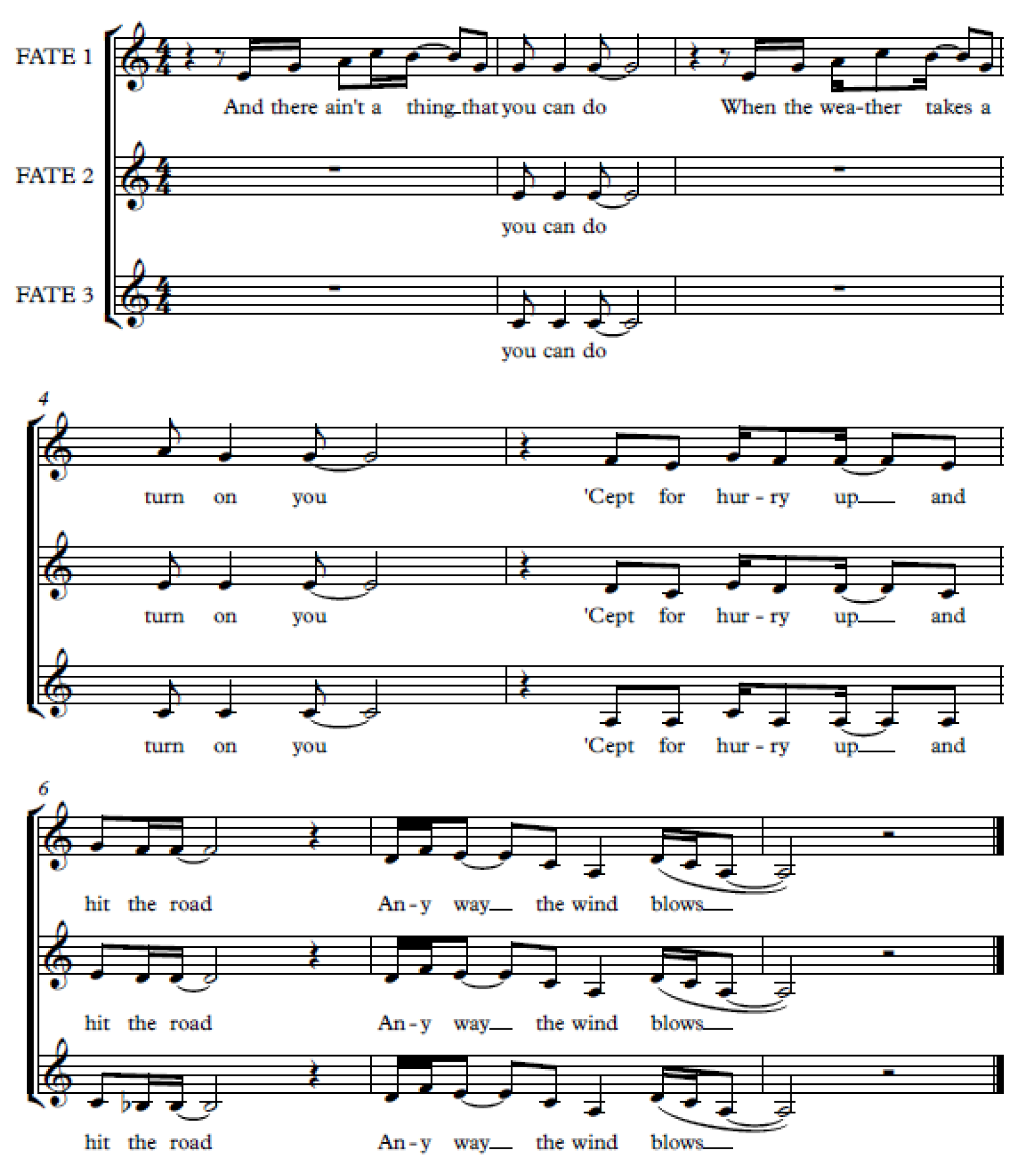
In the musical Hadestown [1], the Fates function as a single character with three voices. This vocal multiplicity expands the variety of musical expression available to the Fates, not only through harmony, but through a carefully crafted mixture of harmonized passages, solos with resting voices, and unison passages (see Figure 1; other examples abound throughout and beyond Hadestown). Prior approaches to the mathematical modeling of voice leading have focused only on harmonized passages, but the judicious use of resting and unison, hardly unique to the Fates in Hadestown, is widespread across many genres. The main goal of this paper is to generalize well-known orbifold models for voice leading to incorporate all three of the passage types listed above as paths in a larger space. A secondary goal is to clarify and elaborate on the idea of orbifold paths and how they relate to geometric and topological structures used to study voice leading.

Some mathematical approaches to voice leading use functions between pitch-class sets as models [2]; others use paths in chord spaces, as in [3,4,5]. The latter approach allows one to make finer, musically relevant distinctions, but to do so with precision requires careful attention to the question of what constitutes a “path” in a chord space. In [6], both “paths” in their usual topological sense and orbifold paths as defined in orbifold theory are considered; the latter are found to be more suitable because they account for the branching that is part of the orbifold structure. In this paper, we extend the idea of orbifold paths to the larger spaces that we introduce, and provide them with algebraic structure via the orbispace path groupoid. We leave the important topic of voice leading size, already explored for chords of differing cardinalities in [7], to later work. We note that the paths we consider are special cases of gestures as studied in [8,9,10]. Other connections via category theory and knot theory can be found in [11]. The general topic of spatialization of music was previously considered in [9,12].

Our task, then, is first of all to define a mathematical space that incorporates both loudness information and pitch-class information for each voice, while allowing for octave equivalence and voice permutation as in prior models. We then need to define a suitable analogue of “orbifold path” in our generalized space, along with concatenation and inverses of such paths that will give the collection of such paths the structure of a groupoid. (Although groups still play a central role, we generalize to groupoids in this work to avoid the musically unnatural requirement that passages begin and end on the same chord.) Next, we need to identify subspaces that correspond to the situations we wish to distinguish—solos with resting voices, passages with two or more voices in unison, and fully harmonized passages. Since in all non-trivial cases, the subspaces of interest will be of dimension at least 4, we need to provide a convenient way to visualize the paths without having to visualize the full extent of the spaces they inhabit. Finally, we need to how our generalized models relate to previously articulated models, focusing primarily on consistency and coherence of connections between them.

In Section 2, we provide the mathematical details, formally defining the spaces, the paths, and the groupoids of interest. In Section 3, we apply the mathematical formalism to musical situations. We first describe in detail how to model voice leadings as groupoid elements. We then explore how different configurations of rests and unisons correspond to interrelating structures of subspaces of our generalized space. We complete Section 3 by introducing singular braids as a means for visualization. In Section 4, we offer some remarks on consistency and connections with other recent work on voice leading. In Section 5, we offer some concluding remarks summarizing the symbiosis of the algebraic and geometric points of view.

2. Materials and Methods

We assume the reader is familiar with the terms group action, orbit, and isotropy, along with the language of basic category theory. For clarity and convenience, we distinguish the terms quotient space, orbit space, orbifold, and orbispace. Let X be a topological space. A quotient space of X is a topological space Q whose points are the equivalence classes of some equivalence relation on X, endowed with the quotient topology which makes the projection $X\to Q$ continuous. An orbit space of X is a quotient space of X for which the equivalence classes are the orbits of some group action on X. If X is a differentiable manifold and G is a group acting properly discontinuously on X, then the orbit space $X/G$ together with the projection $X\to X/G$ is a developable orbifold (sometimes called a good orbifold). The unqualified term orbifold includes spaces in which every point has a neighborhood that is a developable orbifold, but the spaces X and the groups G may vary among such neighborhoods, and the orbifold structures are required to be compatible where the neighborhoods intersect. A developable orbispace is an orbit space $X/G$ together with its corresponding projection $X\to X/G$ (note that X need not be a manifold and G need not act properly discontinuously), and an orbispace is a space in which every point has a neighborhood that is a developable orbispace, and the orbispace structures are compatible where the neighborhoods intersect. All of the orbifolds and orbispaces in this work (and other voice-leading literature) are developable, so for brevity we will usually dispense with the adjective. In most cases, X will be the simply connected universal orbispace cover of the quotient. In all cases, it is extremely important to note that orbifolds and orbispaces carry more information than their corresponding quotient spaces; the projection maps are part of the defining data.

2.1. The Spaces

Following a suggestion in [4], we model loudness as a real number r in the interval $[0,1]$, with 0 representing silence and 1 representing some practical maximum. We could also leave the right endpoint open, using $[0,1)$ or even $[0,\infty )$ for the model, but in all cases it is important to retain the the included left endpoint to achieve our purpose of modeling resting voices. We leave aside the matter of assigning physical units to r (decibels, watts, etc.) or interpreting r in musical terms (p, f, etc.) other than $r=0$ means silence, $r=1$ means as loud as practically possible, and $r_1>r_2$ means $r_1$ is louder than $r_2$.

As in most mathematical approaches to voice leading, we model pitch as a real number $\theta$ which can be interpreted as some affine linear function of the logarithm of frequency. The state of a single voice will thus consist of an ordered pair $(r,\theta )$ whose entries represent loudness and pitch, respectively. A pair $(r,\theta )$ lies a priori in $[0,1]\times \mathbf{R}$, but since all pitches sound alike if the voice is silent, we take the important mathematical step of collapsing the left boundary component $\{(0,\theta )|\theta \in \mathbf{R}\}$ to a single point O, forming the quotient space $C\mathbf{R}$, recognized by topologists as the cone on R. We note that $C\mathbf{R}$ is not a manifold, since no neighborhood of O is homeomorphic to an open subset of ${\mathbf{R}}^2$. Nor is $C\mathbf{R}$ a manifold with boundary, for similar reasons. Note that deleting the cone point O would yield a manifold, but doing so would also obviate our main motivation. We also note that $C\mathbf{R}$, like all cones, is contractible and thus lacking topological structure; a recurring theme in this work is that structure detailed enough to be useful comes not from topology per se but from the additional data with which an orbispace, by definition, comes equipped.

Again following standard approaches, we model octave equivalence via a translation action (music: transposition action) of the infinite cyclic group $\mathbf{Z}$ on $\mathbf{R}$: $k·\theta =\theta +2k\pi$. We choose $2\pi$ as the unit translation distance to suggest the geometric interpretation of $\theta$ as an angle measured in radians (and the interpretation of $(r,\theta )$ as polar coordinates); the equation for musical interpretation is thus $2\pi \mathrm{radians}=1\mathrm{octave}$. We extend this action to $C\mathbf{R}$ by $k·(r,\theta )=(r,k·\theta )$. Note that O is a fixed point for the action since all points of form $(0,\theta )$ are identified with O.

We now form the orbit space $C\mathbf{R}/\mathbf{Z}$ and the natural projection $p:C\mathbf{R}\to C\mathbf{R}/\mathbf{Z}$. Since, as noted above, $C\mathbf{R}$ is not a manifold (and O has infinite isotropy), $C\mathbf{R}/\mathbf{Z}$ cannot properly be called an orbifold. Nevertheless, as we shall see, as an orbispace it retains the path-lifting properties we need in order to proceed. Topologically, $C\mathbf{R}/\mathbf{Z}$ is homeomorphic to the 2-dimensional disk $D^2$ and therefore contractible (but keep in mind the additional structure of the orbispace, in particular the role of O as a singularity). The projection p can be viewed as the the reinterpretation of rectangular coordinates as polar coordinates, which explains our use of the generic symbols r and $\theta$.

The state of a single voice can thus be viewed as a point in the disk $D^2$ endowed with the orbispace structure described above. What we have done is to replace the pitch-class space of prior models, which is a circle $S^1$ having orbifold structure given by $\mathbf{R}\to \mathbf{R}/\mathbf{Z}=S^1$, with pitch-class-with-loudness space $D^2$ having orbispace structure given by $p:C\mathbf{R}\to C\mathbf{R}/\mathbf{Z}$. Note that $D^2$ can be viewed as the cone $C{S}^1$ on pitch-class space, and the natural inclusion $S^1\hookrightarrow C{S}^1$ is compatible with the orbispace structures on both spaces (i.e., natural inclusion commutes with orbispace projection). Again, $C{S}^1$ is contractible and therefore less informative topologically than $S^1$; nevertheless, important information is preserved via transfer to the orbispace structure.

To model n unordered voices, we form the n-fold symmetric product $S{P}^n(D^2)$, which by definition is the orbit space of the action of the symmetric group ${\Sigma }_n$ on ${(D^2)}^n$ given by permuting coordinates. The composite of natural projections

$${(C\mathbf{R})}^n\to {(D^2)}^n\to S{P}^n(D^2)$$

gives an orbispace structure on $S{P}^n(D^2)$ with acting group ${\mathbf{Z}}^n⋊{\Sigma }_n$. Note that n-voice chord space as defined in [5] is $S{P}^n(S^1)$ with orbifold structure given by

$${\mathbf{R}}^n\to {(S^1)}^n\to S{P}^n(S^1)$$

with the same acting group as above. However, $S{P}^n(S^1)$ has the homotopy type of $S^1$ [13], while $S{P}^n(D^2)$ is contractible.

2.2. The Paths

Recall that an ordinary path in a topological space X is a continuous mapping $f:I\to X$, where I is the unit interval $[0,1]$. Standard mathematical terminology calls $f(0)$ the initial point and $f(1)$ the terminal point of f; collectively, they are the endpoints. An ordinary homotopy from a path f to a path g in X is a continuous mapping $H:I\times I\to X$ such that $H(t,0)=f(t)$, $H(t,1)=g(t)$, $H(0,t)=f(0)$, and $H(1,t)=f(1)$ for all $t\in I$; if such an H exists, we say f and g are homotopic (rel endpoints), and we think of H as a continuous deformation from f to g. Note that homotopic paths must have the same initial and terminal points, and these endpoints must remain fixed throughout a homotopy. Homotopy is an equivalence relation on paths, and we denote the equivalence class of a path f by $[f]$. If $f_1$ and $f_2$ are two paths in X such that $f_1(1)=f_2(0)$, then the concatenation (or composition) of $f_1$ and $f_2$ is $f_1\ast f_2$ given by

$$(f_1\ast f_2)(t)=\left\{\begin{array}{cc}{f}_1(2t)\hfill & 0\le t\le 1/2\hfill \\ f_2(2t-1)\hfill & 1/2<t\le 1\hfill \end{array}\right..$$

Concatenation is well defined for homotopy classes of paths, with $[f_1]\ast [f_2]=[f_1\ast f_2]$.

Let $X/G$ be a developable orbispace with projection map $p:X\to X/G$. We will assume X is simply connected, so that all paths in X from a given initial point to a given terminal point are homotopic to one another. We will also assume the following conditions, taken from [14]:

• The projection $p:X\to X/G$ has the path lifting property: if $c:I\to X/G$ is a path, then there is a path $\tilde{c}:I\to X$ such that $p\circ \tilde{c}=c$.
• If $x\in X$, then x has an open neighborhood $U_x$ such that

  (a)

  If $g\in G$ does not belong to the isotropy group $G_x$ of x, then $U_x\cap (g·U_x)=\varphi$;

  (b)

  If a and b are paths in $U_x$ beginning at x and such that $p\circ a$ and $p\circ b$ are homotopic rel endpoints in $X/G$, then there is an element $g\in G_x$ such that $g·a$ and b are homotopic in X rel endpoints.

As noted already in [6], the additional structure of an orbispace invites an enhancement of the notion of a “path” to reflect that structure.

Definition 1.

For a developable orbispace $p:X\to X/G$, a G path is a pair $([\tilde{c}],\gamma )$, where $\tilde{c}$ is an ordinary path in X, and $\gamma \in G$. The initial point of $([\tilde{c}],\gamma )$ is $\tilde{c}(0)$ and the terminal point of $([\tilde{c}],\gamma )$ is $\gamma ·\tilde{c}(1)$.

We note that a pair $(\tilde{c},\gamma )$ is called an $\mathcal{H}$ path in [15]. Passing to path homotopy classes at this juncture is more natural and convenient for our purposes. We now define an equivalence relation on G paths to account for the variability of endpoints in X within fibers over endpoints in $X/G$.

Definition 2.

Let $p:X\to X/G$ be an orbispace, and let $x,y\in X/G$. An orbispace path class is an equivalence class of G paths $([\tilde{c}],\gamma )$ with equivalence relation ∼ given by $([\tilde{c}],\gamma )\sim ([{\tilde{c}}^{\prime }],{\gamma }^{\prime })$ if and only if $p(\tilde{c}(0))=p({\tilde{c}}^{\prime }(0))$, $p(\tilde{c}(1))=p({\tilde{c}}^{\prime }(1))$, and ${\gamma }^{\prime }=\gamma$. The initial point and terminal point of the class of $([\tilde{c}],\gamma )$ are $p(\tilde{c}(0))$ and $p(\gamma ·\tilde{c}(1))$, respectively.

The following theorem gives a useful way to enumerate the orbispace path classes for $p:X\to X/G$.

Theorem 1.

Let $p:X\to X/G$ be an orbispace, and let $x,y\in X/G$. Let $\tilde{x}$ and $\tilde{y}$ be specified points (basepoints) in $p^{-1}(x)$ and $p^{-1}(y)$, respectively. Then the set of orbispace path classes for $p:X\to X/G$ with initial point x and terminal point y is in one-to-one correspondence with the set of G paths for $p:X\to X/G$ with initial point $\tilde{x}$ and terminal point $\tilde{y}$.

Proof. 

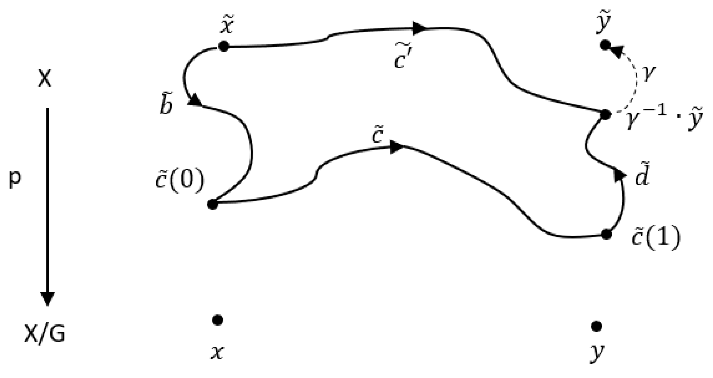
Let $p:X\to X/G$ be an orbispace, and let $([\tilde{c}],\gamma )$ be a representative of an arbitrary orbispace path class with initial and terminal points x and y, respectively. Let $\tilde{x}$ and $\tilde{y}$ be specified points in $p^{-1}(x)$ and $p^{-1}(y)$, respectively. Since (according to our assumptions) X is path connected, there is a path $\tilde{b}$ in X from $\tilde{x}$ to $\tilde{c}(0)$ and a path $\tilde{d}$ from $\tilde{c}(1)$ to ${\gamma }^{-1}·(\tilde{y})$ (see Figure 2). The G path $([\tilde{b}\ast \tilde{c}\ast \tilde{d}],\gamma )$ is equivalent to $([\tilde{c}],\gamma )$ and has initial point $\tilde{x}$ and terminal point $\tilde{y}$, so the orbispace path class represented by $([\tilde{c}],\gamma )$ has a representative with initial point $\tilde{x}$ and terminal point $\tilde{y}$. Now suppose $([{\tilde{c}}^{\prime }],\gamma )$ is another such representative. Then the paths $\tilde{b}\ast \tilde{c}\ast \tilde{d}$ and ${\tilde{c}}^{\prime }$ both have initial point $\tilde{x}$ and terminal point ${\gamma }^{-1}·(\tilde{y})$, so they must be homotopic (since we are assuming X is simply connected). Thus, $([{\tilde{c}}^{\prime }],\gamma )=([\tilde{b}\ast \tilde{c}\ast \tilde{d}],\gamma )$, so the representative $([\tilde{b}\ast \tilde{c}\ast \tilde{d}],\gamma )$ is unique. □

The preceding theorem may appear at first glance to be a mere technical sideshow, but in actuality it plays a profound role in connecting orbifold theory with voice leading. Dragomir, in [15] as well as private communications, has repeatedly stressed the importance of basepoint selection in making the study of orbifold paths precise and coherent. On the other hand, fundamental domains for quotient spaces are important tools for depicting and describing voice leading [16]. As will be noted later, a choice of basepoint in each fiber $p^{-1}(x)$ in X is exactly the same as a choice of fundamental domain in X for $p:X\to X/G$.

2.3. The Groupoids

Recall that a groupoid is a small category in which every morphism is an isomorphism. One can think of a groupoid as a generalization of a group wherein not every pair of elements can be combined using the operation. Two important examples for our purposes are tree groupoids and fundamental groupoids of topological spaces. If S is a set (in the mathematical sense), the tree groupoid $T(S)$ on S is the groupoid whose objects are the elements of S and for which there is exactly one morphism for each ordered pair of objects. If X is a topological space, the fundamental groupoid $\pi (X)$ of X is the groupoid whose objects are the points of X and whose morphisms from x to y are the (ordinary) path homotopy classes of paths from x to y.

Definition 3.

If Γ is a groupoid and G is a group acting on Γ (on the left), then the semidirect product $\mathsf{\Gamma }⋊G$ of Γ and G is the groupoid whose objects are the objects of Γ, whose morphisms from x to y consist of pairs $(\gamma ,g)$ where Γ is a morphism in Γ from x to $g^{-1}·y$ and $g\in G$, and for which concatenation of morphisms $(\gamma ,g)$ from x to y and $(\delta ,h)$ from y to z is given by $(\gamma ,g)\ast (\delta ,h)=(\gamma \ast g^{-1}·\delta ,hg)$.

Our definition of $\mathsf{\Gamma }⋊G$ is a slight variation of the one given in [14] (where g acts on the initial point rather than the terminal point of $\gamma$); the variation is for agreement with the formalism of $\mathcal{H}$ paths given in [15].

Let $([\tilde{c}],\gamma )$ and $([\tilde{d}],\delta )$ be G paths in $p:X\to X/G$ with $\tilde{d}(0)=\gamma ·\tilde{c}(1)$. We define the concatenation of $([\tilde{c}],\gamma )$ and $([\tilde{d}],\delta )$ to be $([\tilde{c}],\gamma )\ast ([\tilde{d}],\delta )=([\tilde{c}\ast {\gamma }^{-1}·\tilde{d}],\delta \gamma )$. The inverse of $([\tilde{c}],\gamma )$ is $([\gamma ·{\tilde{c}}^{-1}],{\gamma }^{-1})$, where ${\tilde{c}}^{-1}(t)=\tilde{c}(1-t)$. The concatenation of the orbispace path classes represented by $([\tilde{c}],\gamma )$ and $([\tilde{d}],\delta )$ is the orbispace path class of $([\tilde{c}],\gamma )\ast ([\tilde{d}],\delta )$, and the inverse of the orbispace path class represented by $([\tilde{c}],\gamma )$ is the orbispace path class of $([\gamma ·{\tilde{c}}^{\prime }],{\gamma }^{-1})$.

Theorem 2.

Concatenation and inverses are well defined for orbispace path classes.

Proof. 

Let $([\tilde{c}],\gamma )$ and $([\tilde{d}],\delta )$ be G paths in $p:X\to X/G$ with $\tilde{d}(0)=\gamma ·\tilde{c}(1)$. Let $([{\tilde{c}}^{\prime }],\gamma )$ and $([{\tilde{d}}^{\prime }],\delta )$ be two other G paths in $p:X\to X/G$ with $p({\tilde{c}}^{\prime }(0))=p(\tilde{c}(0))$, $p({\tilde{c}}^{\prime }(1))=p(\tilde{c}(1))$, $p({\tilde{d}}^{\prime }(1))=p(\tilde{d}(1))$, and ${\tilde{d}}^{\prime }(0)=\gamma ·{\tilde{c}}^{\prime }(1)$. We have

$$([\tilde{c}],\gamma )\ast ([\tilde{d}],\delta )=([\tilde{c}\ast {\gamma }^{-1}·\tilde{d}],\delta \gamma )$$

and

$$([{\tilde{c}}^{\prime }],\gamma )\ast ([{\tilde{d}}^{\prime }],\delta )=([{\tilde{c}}^{\prime }\ast {\gamma }^{-1}·{\tilde{d}}^{\prime }],\delta \gamma )$$

and since

$$p(\tilde{c}\ast {\gamma }^{-1}·\tilde{d}(0))=p(\tilde{c}(0))=p({\tilde{c}}^{\prime }(0))=p({\tilde{c}}^{\prime }\ast {\gamma }^{-1}·{\tilde{d}}^{\prime }(0))$$

and

$$p(\tilde{c}\ast {\gamma }^{-1}·\tilde{d}(1))=p({\gamma }^{-1}·\tilde{d}(1))=p({\gamma }^{-1}·({\tilde{d}}^{\prime }(1))=p({\tilde{c}}^{\prime }\ast {\gamma }^{-1}·{\tilde{d}}^{\prime }(1))$$

we obtain $([\tilde{c}],\gamma )\ast ([\tilde{d}],\delta )\sim ([{\tilde{c}}^{\prime }],\gamma )\ast ([{\tilde{d}}^{\prime }],\delta )$.

For inverses, we have

$${([\tilde{c}],\gamma )}^{-1}=([\gamma ·{\tilde{c}}^{-1}],{\gamma }^{-1})$$

and

$${([{\tilde{c}}^{\prime }],\gamma )}^{-1}=([\gamma ·{({\tilde{c}}^{\prime })}^{-1}],{\gamma }^{-1}),$$

and since

$$p(\gamma ·{\tilde{c}}^{-1}(0))=p(\tilde{c}(1))=p({\tilde{c}}^{\prime }(1))=p(\gamma ·{({\tilde{c}}^{\prime })}^{-1}(0))$$

and

$$p(\gamma ·{\tilde{c}}^{-1}(1))=p(\tilde{c}(0))=p({\tilde{c}}^{\prime }(0))=p(\gamma ·{({\tilde{c}}^{\prime })}^{-1}(1))$$

we have ${([\tilde{c}],\gamma )}^{-1}\sim {([{\tilde{c}}^{\prime }],\gamma )}^{-1}$. □

Definition 4.

The orbispace path groupoid ${\pi }^{orb}(X/G)$ of an orbispace $p:X\to X/G$ is the category whose objects are the points of $X/G$, and the morphisms of which are the orbispace path classes with concatenation as defined above. The category ${\pi }^{orb}(X/G)$ is a groupoid since every orbispace path class has an inverse.

The orbispace path groupoid can be regarded as a refinement of the fundamental groupoid of a space, analogous to how the orbifold fundamental group is a refinement of the ordinary fundamental group of a space. We use the term “orbispace path groupoid” instead of “orbifold fundamental groupoid” to help prevent inaccurate conflation of terms of the sort that occurs in [17] with “fundamental group" and “orbifold fundamental group”.

Note that G acts on $T(X/G)$, the tree groupoid on $X/G$. The orbispace path groupoid has the following useful characterization.

Theorem 3.

The orbispace path groupoid ${\pi }^{orb}(X/G)$ is isomorphic to $T(X/G)⋊G$.

Proof. 

First note that ${\pi }^{\mathrm{o}rb}(X/G)$ and $T(X/G)⋊G$ have the same objects, namely the points of $X/G$. Next note that the morphisms of $T(X/G)⋊G$ from x to y are in bijective correspondence with pairs $((x,g^{-1}·y),g)$ since there is only one morphism from x to $g^{-1}·y$. However, G acts trivially on $X/G$, so the morphisms from x to y are pairs $((x,y),g)$, in bijective correspondence with members of G.

On the other hand, morphisms of ${\pi }^{\mathrm{o}rb}(X/G)$ from x to y are equivalence classes of G paths $([\tilde{c}],g)$ where $\tilde{c}$ is a path in X whose initial and terminal points are in the fibers of x and y, respectively. Two such pairs are equivalent if the images of their endpoints in $X/G$ agree and their group elements agree, so again the equivalence classes are in bijective correspondence with pairs $((x,y),g)$ where $g\in G$.

Finally, we note that concatenation in both groupoids is given by

$$((x,y),g)\ast ((y,z),h)=((x,z),hg).$$

(Note that this shows that concatenation in the orbispace path groupoid is completely captured by the group operation in the acting group. Moreover, any element $((x,y),g)$ of ${\pi }^{\mathrm{o}rb}(X/G)$ can be factored as $((x,y),1)\ast ((y,y),g)$, so morphisms between specified objects correspond to group elements.) □

Remarkably, the mathematically motivated characterization of elements of ${\pi }^{\mathrm{o}rb}(X/G)$ as products of the form $((x,y),1)\ast ((y,y),g)$ in $T(X/G)⋊G$ is the mathematical formulation of the musically motivated method described on pages 122, 130, 135, and elsewhere in [17] (which in turn references earlier work of Roederer) for dealing with voice leadings between different chords. In that method, one chooses an arbitrary, fixed voice leading between the two chords, and factors any given voice leading between them as the chosen voice leading followed by a voice leading from the second chord to itself. This unforced confluence of the mathematical and musical points of view is an encouraging sign that the use of geometric topology in music theory is a promising and worthwhile endeavor.

The orbispace path groupoid is an orbispace invariant. Additionally—and importantly for our purposes—it is functorial in the sense that a morphism of orbispaces induces a morphism of the associated orbispace path groupoids. Functoriality is particularly important when considering the inclusion maps of the various musically relevant subspaces (and subspaces of subspaces) of our generalized chord spaces. A fortiori, functoriality can be used to mediate between any family of geometrical or topological topological spaces used to model any collection of musical parameters, and any corresponding families of algebraic objects used to model relationships (transformations, gestures, etc.) between sets of parameters.

3. Results

In this section, we apply the mathematical framework described above to musical situations.

3.1. Voice Leadings as Groupoid Elements

We now describe and demonstrate a procedure for associating groupoid elements with voice leadings in music. In light of Theorem 1, a crucial preliminary step in the procedure is a choice, for each point x in $X/G$, of a specific basepoint ${\tilde{x}}_0$ in the fiber $p^{-1}(x)$. In the musical situation of chord space (OP space) with loudness, $X={(C\mathbf{R})}^n$, $G={\mathbf{Z}}^n⋊{\Sigma }_n$, and $X/G=S{P}^n(D^2)$. We can think of an element x of $X/G$ as a chord, but it is important to keep in mind the following differences between “chords” in the usual sense and elements of $X/G$. First, an element of $X/G$ is an equivalence class of n-tuples of pairs $(r,\theta )$ where $r\in [0,1]$ represents loudness and $\theta \in \mathbf{R}$ represents pitch, so loudness is part of the data for each entry, and two entries with the same pitch (or pitch class) but different loudness are considered distinct. Second, it is possible for two entries to be equal (or equivalent), so we retain multiplicities (doublings) as part of the data (e.g., the 4-tuples (C, C, E, G) and (C, E, G, G) (with all entries having equal loudness) represent distinct “chords” in our context). Thus, a chord in the sense of an element of $X/G$ is an unordered multiset of n pairs, $\{(r_1,{\theta }_1),\dots ,(r_n,{\theta }_n)\}$.

A specific choice of basepoint ${\tilde{x}}_0\in X$ for a chord $x\in X/G$ is a choice of a specific voicing of the chord x—that is, a specific ordering (part assignment) of the pairs in x and, for each pair, a choice of octave (register). As noted above, it is an interesting and important fact that a collection of such choices for every element of $X/G$ is the same as a choice of a fundamental domain for the action of G on X. Insofar as fundamental domains are used in [16,17] to study quotient spaces, basepoint selection should appear as a natural and familiar step. It is also important to note that basepoint selection is to be done once and remain unchanged throughout a discussion.

There are infinitely many ways to make a selection of basepoints (or fundamental domain) in $X={(C\mathbf{R})}^n$. In the examples that follow, we will choose, for a given chord $\{(r_1,{\theta }_1),\dots ,(r_n,{\theta }_n)\}$, the representative with each ${\theta }_i$ in the octave ascending from middle C, with the pairs put in dictionary order (i.e., the relation given by $(r_i,{\theta }_i)<(r_j,{\theta }_j)$ if $r_i<r_j$, or if $0<r_i=r_j$ and ${\theta }_i<{\theta }_j$; recall $(0,{\theta }_i)=(0,{\theta }_j)$ for all ${\theta }_i,{\theta }_j$).

Here is the procedure for associating an element of the groupoid ${\pi }^{\mathrm{o}rb}(X/G)\cong T(X/G)⋊G$ to a given voice leading taken from actual music (see Figure 3 for a schematic illustration). A voice leading in actual music is specified by part assignments (voicings) $\tilde{x},\tilde{y}\in X$ for the initial and terminal chords $x,y\in X/G$; such a pair of voicings represents an equivalence class of paths under the uniform operation of G on paths in X.

• Choose an element ${\gamma }_0$ of G that moves the given initial voicing $\tilde{x}$ to the basepoint voicing ${\tilde{x}}_0$ of the initial chord x (i.e., ${\gamma }_0$ that moves $\tilde{x}$ into the chosen fundamental domain).
• Apply ${\gamma }_0$ to the given terminal voicing $\tilde{y}$ of the terminal chord y, effectively completing the uniform operation of ${\gamma }_0$ on the path from $\tilde{x}$ to $\tilde{y}$. Note that since the path may end in a fundamental domain other than the one where it originated, ${\gamma }_0·\tilde{y}$ will not necessarily be equal to the basepoint voicing ${\tilde{y}}_0$ of y (see Figure 3).
• Since $\tilde{y}$, ${\gamma }_0·\tilde{y}$, and ${\tilde{y}}_0$ all lie in the fiber over x and hence in the same orbit under the action of G (i.e., they are all voicings of the same chord), we can choose $\gamma \in G$ such that $\gamma ·({\gamma }_0·\tilde{y})={\tilde{y}}_0$ (i.e., $\gamma$ that moves ${\gamma }_0·\tilde{y}$ into the chosen fundamental domain).
• The associated element of the groupoid ${\pi }^{\mathrm{o}rb}(X/G)\cong T(X/G)⋊G$ is then $(x,y,\gamma )$.

Note that the element $\gamma$ of the acting group takes the terminal point ${\gamma }_0·\tilde{y}$ back to the preferred fundamental domain, so if we want to think in terms of the forward motion of a voice leading, i.e., taking an initial voicing forward to a terminal voicing, then the element to associate with the voice leading is ${\gamma }^{-1}$. Use of the forward action is more intuitive musically, but use of the backward action is consistent with previously established conventions in [14,15]. Simple awareness of the distinction should be sufficient to avoid confusion.

For an example, consider the fifth measure of the Hadestown example given above. The first three chords represent two concatenated voice leadings (see Figure 4). We will make the simplifying assumption that loudness is equal, constant, and non-zero for all voices, and thereby omit loudness from the notation. Likewise, since all multiplicities in this example are 1 (i.e., there is no doubling), we will simply designate the three underlying chords in $X/G$ by Dm, Am, and C. In X (where order matters), we will specify voicings using the ordering (Fate 3, Fate 2, Fate 1), so that the three given voicings are (A3, D4, F4), (A3, C4, E4), and (C4, E4, G4). Recall that that our (arbitrary but fixed) choice for basepoint voicing of each chord has every pitch in the octave ascending from middle C (C4). For clarity, we use two-row notation to specify permutations.

• The basepoint voicing of the first chord is (D4, F4, A4), so the element ${\gamma }_0\in G$ taking the first given voicing to the basepoint voicing is the cyclic permutation $\left(\begin{array}{ccc}1& 2& 3\\ 3& 1& 2\end{array}\right)$ followed by raising the third voice by an octave: ${\gamma }_0=(0,0,1)\circ \left(\begin{array}{ccc}1& 2& 3\\ 3& 1& 2\end{array}\right)$.
• We apply ${\gamma }_0$ to the second voicing to obtain (C4, E4, A4), which we note in this case happens to be the basepoint voicing.
• The corresponding element $\gamma \in G$ for this voice leading is thus the identity element $1=(0,0,0)\circ \left(\begin{array}{ccc}1& 2& 3\\ 1& 2& 3\end{array}\right)$.
• We therefore associate the groupoid element (Dm, Am, 1) to the first voice leading.

Now consider the second voice leading, represented by the voicing (A3, C4, E4) followed by the voicing (C4, E4, G4).

• To move (A3, C4, E4) to the basepoint voicing, we again need to apply ${\gamma }_0=(0,0,1)\circ \left(\begin{array}{ccc}1& 2& 3\\ 3& 1& 2\end{array}\right)$.
• We apply ${\gamma }_0$ to (C4, E4, G4) to obtain (E4, G4, C5), which we note is not the basepoint voicing.
• To move (E4, G4, C5) to the basepoint voicing (C4, E4, G4), we apply the group element $(-1,0,0)\circ \left(\begin{array}{ccc}1& 2& 3\\ 2& 3& 1\end{array}\right)$.
• Thus, we associate the groupoid element (Am, C, $(-1,0,0)\circ \left(\begin{array}{ccc}1& 2& 3\\ 2& 3& 1\end{array}\right)$) to the second voice leading. Note that the “forward” version would take the basepoint voicing of Am to the basepoint voicing of C and then apply the inverse of the associated group element, which is $\left(\begin{array}{ccc}1& 2& 3\\ 3& 1& 2\end{array}\right)\circ (1,0,0)$. This illustrates the remark made above on factoring a given voice leading between two different chords as a fixed, chosen (i.e., basepoint) voice leading from the first chord to the second, followed by a voice leading of the second chord to itself.

The concatenation of the two voice leadings is represented by the voicing (A3, D4, F4) followed by (C4, E4, G4) (just omit the middle voicing!), and the associated groupoid element is

$$(\mathrm{Am},\mathrm{C},(-1,0,0)\circ \left(\begin{array}{ccc}1& 2& 3\\ 2& 3& 1\end{array}\right))\circ (\mathrm{Dm},\mathrm{Am},1)=(\mathrm{Dm},\mathrm{C},(-1,0,0)\circ \left(\begin{array}{ccc}1& 2& 3\\ 2& 3& 1\end{array}\right)).$$

Note that the concatenation of the groupoid elements agrees with what we would get by running the procedure on the sequence directly.

In the procedure given above, we have noted that the existence of ${\gamma }_0$ and $\gamma$ in G taking $\tilde{x}$ to ${\tilde{x}}_0$ and ${\gamma }_0·\tilde{y}$ to ${\tilde{y}}_0$, respectively, is assured since the respective points are in the same respective orbits, but we have said nothing about whether ${\gamma }_0$ or $\gamma$ is unique. In fact, if both $\tilde{x}$ and $\tilde{y}$ have trivial isotropy groups (as in the examples above), then ${\gamma }_0$ and $\gamma$ are unique. On the other hand, if either endpoint has non-trivial isotropy, then ${\gamma }_0$ and $\gamma$ are not unique. The possibility of associating multiple, distinct members of the groupoid ${\pi }^{\mathrm{orb}}(X/G)$ to the same pair of voicings in X is one of the main differences between the orbispace path approach to voice leading and other approaches. As noted in [17], this possibility is occasionally counterintuitive, but it is a natural, musically relevant consequence of the idea of “continuous transformations” articulated in [4], and adopted in [5]. We demonstrate this with an example.

Consider the voice leading from the sixth to the seventh measure of the Hadestown example above, represented by the sequence of voicings (B♭3, D4, F4), (D4, D4, D4) (ignoring, for now, the rests between the two voicings, and assuming again that the loudness is equal and constant for all entries). The second chord consists of a single pitch class with multiplicity 3. The corresponding isotropy group is isomorphic to ${\Sigma }_3$, which has six elements. The element ${\gamma }_0=(0,0,1)\circ \left(\begin{array}{ccc}1& 2& 3\\ 3& 1& 2\end{array}\right)$ takes the initial point to the basepoint (D4,F4,B♭4), and takes the terminal point (D4, D4, D4) to (D4, D4, D5). Thus, we could choose $(0,0,-1)\circ 1$ as the element $\gamma$ to take (D4, D4, D5) to (D4, D4, D4), but there are five other choices: $(0,0,-1)\circ \left(\begin{array}{ccc}1& 2& 3\\ 2& 1& 3\end{array}\right)$, $(0,-1,0)\circ \left(\begin{array}{ccc}1& 2& 3\\ 1& 3& 2\end{array}\right)$, $(0,0,-1)\circ \left(\begin{array}{ccc}1& 2& 3\\ 3& 1& 2\end{array}\right)$, $(-1,0,0)\circ \left(\begin{array}{ccc}1& 2& 3\\ 3& 2& 1\end{array}\right)$, and $(-1,0,0)\circ \left(\begin{array}{ccc}1& 2& 3\\ 2& 3& 1\end{array}\right)$. The six possibilities for $\gamma$, corresponding to the six elements of ${\Sigma }_3$, account for the existence of paths in the homotopy class of paths from (B♭3, D4, F4) to (D4, D4, D4) during which each of the corresponding voice permutations can occur. For example, a path from (B♭3, D4, F4) to (D4, D4, D4) could visit the point (F4,D4,B♭3) en route. Parsing the path into a concatenation with (F4, D4, B♭3) as intermediate point allows factorization of the corresponding element of ${\pi }^{\mathrm{orb}}(X/G)$ as

$$(\mathrm{B}♭,\mathrm{B}♭,(0,-1,1)\circ \left(\begin{array}{ccc}1& 2& 3\\ 1& 3& 2\end{array}\right))\circ (\mathrm{B}♭,\left\{\mathrm{D}4,\mathrm{D}4,\mathrm{D}4\right\},(0,0,-1)\circ 1)$$

which reduces to $(\mathrm{B}♭,\left\{\mathrm{D}4,\mathrm{D}4,\mathrm{D}4\right\},(0,-1,0)\circ \left(\begin{array}{ccc}1& 2& 3\\ 1& 3& 2\end{array}\right))$, one of the possibilities listed above.

Recognizing that the intermediate point could have been literally any point in X (and indeed, the path presented has $(O,O,O)$ (all voices resting) as an intermediate point, with isotropy group all of G), the factorization could have had as its first factor any morphism of ${\pi }^{\mathrm{orb}}(X/G)$ emanating from a B♭ chord. The product morphism, however, must be one of the groupoid elements listed above. The salient fact here is that each of those elements is “musically observable” in the parlance of [17] via the presence of an appropriate intermediate point. The plethora of possible intermediate points is a defining feature of, and the main motivation for, “continuous transformations” as presented in [4], and a feature of homotopy classes of paths. It is possible to restrict the set of possible intermediate points for paths and homotopy classes, a topic we will address in subsequent sections, but to suppress completely the freedom homotopy affords between endpoints is to abandon the continuous model.

3.2. Chords with Rests or Doublings, and Their Associated Subspaces

There are several subspaces of our generalized chord space $X/G=S{P}^n(D^2)$ that are of musical interest. The first distinction we make is between regular points and singular points.

Definition 5.

A point x in the orbispace $X/G$ with projection map $p:X\to X/G$ is a singular point if there exists $\tilde{x}\in p^{-1}(x)$ and $g\ne 1$ in G such that $g·\tilde{x}=\tilde{x}$. A point in $X/G$ is a regular point if it is not a singular point.

In the language of group actions, the singular points are the images of points in X with non-trivial isotropy groups. For our generalized chord space $S{P}^n(D^2)$ with projection map $p:{(C\mathbf{R})}^n\to S{P}^n(D^2)$, there are two kinds of singular points: chords with rests and chords with multiplicities (music: doublings). If we denote a generic point in $S{P}^n(D^2)$ by $\{x_1,x_2,\dots ,x_n\}$ (an unordered collection of n points in $D^2$), then a chord with rests is a point with at least one $x_i=O$, and a chord with multiplicities is a point with $x_i=x_j$ for at least one pair of distinct indices i and j. Note that it is possible for a point in $S{P}^n(D^2)$ to be both a chord with rests and a chord with multiplicities (as in, for example, the first measure of the Hadestown excerpt above). Additionally note that unison chords with $n>1$, such as those in the last two measures of the Hadestown example, are a special case of chords with multiplicities. Finally, we note that although chords with multiplicities have been recognized and studied previously using the orbifold models $S{P}^n(S^1)$, the ability to model chords with rests in the continuous context is new with the $S{P}^n(D^2)$ models.

We now introduce some notation that will facilitate discussion of subspace structures. First, we will denote by $C^n$ our model for n-voice chord space with loudness ($=X/G=S{P}^n(D^2)$). Next, we will denote by $C_k^n$ the subspace of $C^n$ consisting of all n-voice chords with at most $k\le n$ distinct parts (i.e., elements of $D^2$, loudness together with pitch class). We will denote by $C_{k,l}^n$ the subspace of $C_k^n$ consisting of all n-voice chords with exactly l distinct parts, where $l\le k$. Finally, we will denote by $C_{k,l}^{n=m_1+\dots +m_l}$ the subspace of $C_{k,l}^n$ consisting of all n-voice chords with exactly l distinct parts and specific multiplicities $m_1\le \dots \le m_l$ for those parts (i.e., a specific l partition of n).

As an example, consider the passage shown in Figure 5, in which we assume all voices have equal loudness at all times. The first chord lies in $C_1^4$ (all voices in unison). In the second half of the first measure, the passage moves into $C_{2,2}^{4=2+2}$ (two distinct parts, with two voices on each). At the end of the second measure, it moves into $C_{3,3}^{4=1+1+2}$ (three distinct parts, with one doubled), and in the fourth measure, into $C_{4,4}^{4=1+1+1+1}$ (all voices on distinct parts and none resting: a regular point). In the last measure, it moves back into $C_{3,3}^{4=1+1+2}$.

The notation reflects the ability of the model to make subtle distinctions in voice leading. For example, if the tenor were instead to remain in unison with the alto except in the fourth measure, then second subspace visited would be $C_{2,2}^{4=1+3}$ rather than $C_{2,2}^{4=2+2}$.

Rather than introduce even more notation for subspaces of chords with rests, we will identify the subspace $\{\{x_1,\dots ,x_n\}\in C^n|\mathrm{at}\mathrm{most}r\mathrm{entries}\ne O\}$ with $C^r$, where $r<n$. Thus, for example, the first measure of the Hadestown example can be regarded as lying in $C^1\subset C^3$. With these identifications and the notation given above, we obtain the following double filtration of $C^n$ by singular subspaces:

$$\begin{array}{ccccccccc}{C}^1& \subset & C^2& \subset & C^3& \subset & \cdots & \subset & C^n\\ & & \cup & & \cup & & \cdots & & \cup \\ & & C_1^2& \subset & C_2^3& \subset & \cdots & \subset & C_{n-1}^n\\ & & & & \cup & & & & \cup \\ & & & & C_1^3& \subset & \cdots & \subset & C_{n-2}^n\\ & & & & & & & & \cup \\ & & & & & & & & ⋮\\ & & & & & & & & \cup \\ & & & & & & & & C_1^n\end{array}$$

It is interesting and important to note that while $C^r$ and $C_r^s$ (where $s>r$; focus on descending diagonals in the double filtration) are similar in the sense that they both have the same maximal number of parts, they are different subspaces of $C^n$. In particular, $C_r^s$ has a richer substructure due to a greater variety of multiplicities (or cardinalities, as in the OPTIC acronym of [5]) assignable to the parts.

To discuss the multiplicity-based substructure of $C_r^n$, we first give a clarifying reminder about use of term “partition” in two distinct, mathematically standard ways. A partition of n means an expression of n as a sum of positive integers, e.g., $n=m_1+\cdots +m_r$ (in our context the $m_i$ are multiplicities; mathematically, the $m_i$ are called parts which fits unusually well with the musical meaning of parts). A partition of $C_r^n$ means a decomposition of $C_r^n$ into a union of disjoint subsets, e.g., $C_r^n=C_{r,1}^n\cup \cdots \cup C_{r,r}^n$. The partitions of n serve to index the subsets comprising a musically relevant partition of $C^n$. Specifically, we refine the partition $C_r^n=C_{r,1}^n\cup \cdots \cup C_{r,r}^n$ by noting that each $C_{r,i}^n$ is itself partitioned into subsets $C_{r,i}^{n=m_1+\cdots +m_i}$, where $n=m_1+\cdots +m_i$ runs through all i partitions of n.

As an example, consider $C_3^4$, chords with four voices and three or fewer distinct entries. We have the partition

$$C_3^4=C_{3,3}^{4=1+1+2}\cup C_{3,2}^{4=1+3}\cup C_{3,2}^{4=2+2}\cup C_{3,1}^{4=4}.$$

We note that the two subsets with the $3,2$ subscript are not only disjoint, but separated in the topological sense, meaning that there is no path in $C_3^4$ from $C_{3,2}^{4=1+3}$ to $C_{3,2}^{4=2+2}$ that does not pass through either $C_3^4=C_{3,3}^{4=1+1+2}$ or $C_{3,1}^{4=4}$. Musically, this means that to get (via a continuous path in 4-voice space with no more than 3 parts) from a chord with three voices on one part and one voice on another part to a chord with 2 voices on each of two parts, there must either be a time when there is exactly 1 part or a time when there are exactly 3 parts. The situation can be visualized if we restrict to the subspace in which all voices have constant loudness of 1. The intersection of $C_3^4$ with this subspace is then the product of the surface of a tetrahedron with an interval, with ends identified after a cyclic permutation of the faces as pictured in [16]. The subspace $C_{3,2}^4$ is the product of an interval with the union of the interiors of the edges of the tetrahedron, with identifications of the ends forming a pair of open Möbius strips separated by a common boundary, which is $C_{3,1}^4$. A path from one of the strips to the other must either pass through the boundary, or through the product of an interval with the interiors of the faces of the tetrahedron (with end faces permuted and identified), which is $C_{3,3}^4$. Visualization without restricting to a constant-loudness subspace is problematic, since all of the dimensions are doubled. We address this problem in the next subsection.

The preceding example illustrates a more general fact.

Theorem 4.

Let n, k, and l be positive integers with $n\ge k\ge l$ and the number of l partitions of n at least 2. Then $C_{k,l}^n$ is not path connected.

Proof. 

Let n, k, and l be as described in the theorem statement. Let $n=m_1+\cdots +m_l$ and $n=m_1^{\prime }+\cdots +m_l^{\prime }$ be two distinct l partitions of n. Let $(x_1^0,\cdots ,x_n^0)$ and $(x_1^1,\cdots ,x_n^1)$ be representatives in ${(D^2)}^n$ of points in $C_{k,l}^{n=m_1+\cdots +m_l}$ and $C_{k,l}^{n=m_1^{\prime }+\cdots +m_l^{\prime }}$, respectively. Let $x:[0,1]\to {(D^2)}^n$ be a path from $(x_1^0,\cdots ,x_n^0)$ to $(x_1^1,\cdots ,x_n^1)$; with coordinate paths $x_1(t),\dots ,x_n(t)$ for $0\le t\le 1$.

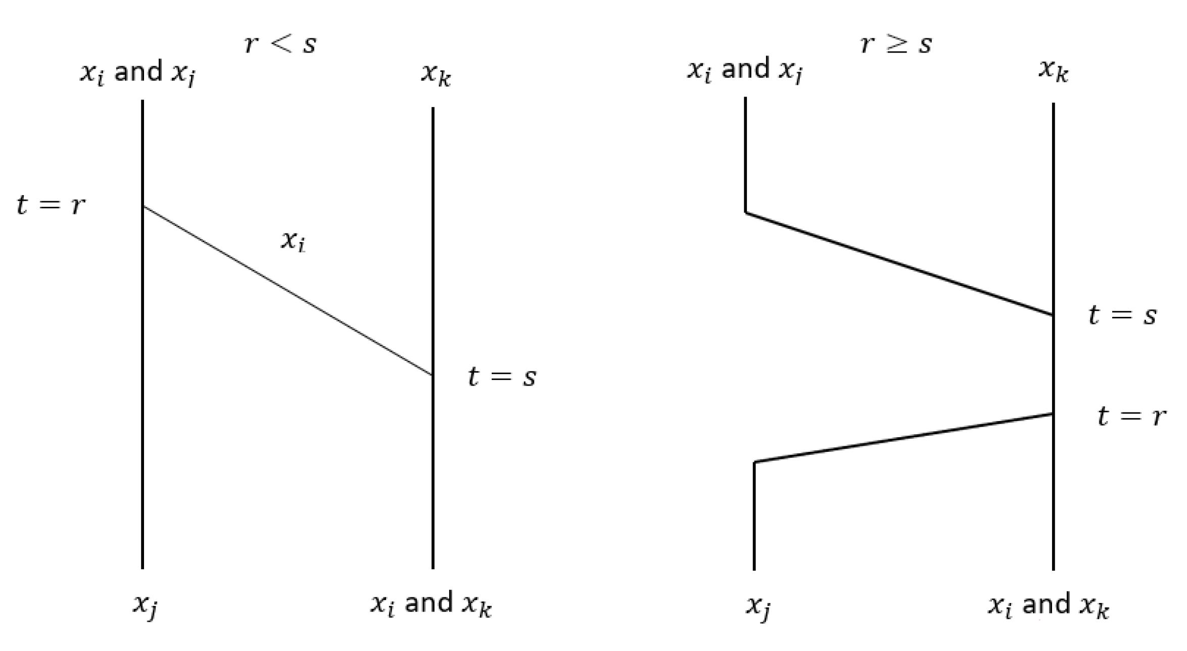
For the distribution of multiplicities to change, at least one coordinate path $x_i$ must depart from its starting part shared with some $x_j$, $j\ne i$, and join a different part shared with some $x_k$, $k\ne i$, $k\ne j$ (see Figure 6). Thus, there exist times r and s such that $x_i(t)=x_j(t)$ for $0\le t\le r$ and $x_i(t)\ne x_j(t)$ for $t>r$, and $x_i(t)\ne x_k(t)$ for $0\le t\le s$ and $x_i(t)=x_k(t)$ for $t>s$. If $r<s$, then for $r<t<s$$x(t)$ has $l+1$ parts. If $r\ge s$, then for $s\le t\le r$$x(t)$ has $l-1$ parts. Thus, the path x must pass through $C_{k,l+1}^n$ or $C_{k,l-1}^n$. If other departures and/or joinings occur simultaneously, the number of parts may be increased or decreased further, but in such cases it cannot remain at l for all t in $[0,1]$. □

The significance of the preceding discussion and theorem has less to do with particular musical passages—after all, the path constructed in the proof of the theorem above may have only momentary, “unobservable” contact with $C_{k,l+1}^n$ or $C_{k,l-1}^n$—and more to do with its suggestion that $C_k^n$ can be endowed with a structure similar to that of a cell complex, with $C_k^n$ as its $2k$-skeleton (k-skeleton if restricted to a constant-loudness subspace), and l partitions of n corresponding to the interiors of $2l$-dimensional cells (l-dimensional for constant loudness). These cell interiors are the subspaces $C_{k,l}^{n=m_1+\cdots +m_l}$, which correspond musically to n voices assigned to l parts with $m_i$ voices on the i-th part.

One might expect that restricting a path (and its homotopy class) to $C_k^n$, for $k<n$, would also restrict the ability to make“musically observable” distinctions between different choices of group elements taking the terminal point of the path to the basepoint. However, if $k>1$, the availability of points in $C_{k,1}^n$ (musically, all voices in unison) makes the distinctions possible. Consider, for example, the chord in $C_2^3$ represented by (G4, G4, B4), and a path in ${(C\mathbf{R})}^3$ that starts and ends on this representative. Assuming all loudness levels equal, non-zero, and constant, there are two group elements corresponding to the path, the identity and the permutation that interchanges the first two entries. If the path (and its homotopy class) is constrained such that its image in $C^3$ must remain in $C_2^3$, no regular point is available as an intermediate point, but visiting the sequence of points (G4, G4, G4), (G4, B4, G4), (G4, G4, G4) can be accomplished within $C_2^3$ and is sufficient to distinguish between the two choices.

On the other hand, if $k=1$, the strategy of having the path visit $C_1^n$ and then return to $C_{k,l}^n$ (where $l>1$) to swap voices does not work. Hence, for voice leadings constrained to remain in $C_1^n$ (such as the one represented by a path beginning and ending at (A4, A4)), distinctions between group elements in the isotropy subgroup are indeed unobservable. More generally, restricting to a subspace $C_{k,k}^n$ with exactly k distinct parts can also prevent voice swapping and render some distinctions unobservable.

We have already mentioned “constant-loudness” subspaces. At this point, we observe more explicitly that the subspace of $S{P}^n(D^2)$ consisting of chords for which the loudness for all voices is fixed at any constant $\lambda$ such that $0<\lambda \le 1$ can be identified with the chord space without loudness $S{P}^n(S^1)$ that has been studied extensively in [5,16,17]. We will revisit these subspaces in each of the next two subsections.

3.3. Visualization and Braids

Since the dimension of $S{P}^n(D^2)$ is $2n$, visualization of the full extent of the space is only feasible when $n=1$. There are various strategies for reducing the dimension to enable visualization, each one making trade-offs to favor particular analytical motivations. One such strategy is restriction to a constant-loudness subspace, enabling visualization for $n=2$ and $n=3$, at the cost of visualization (and modeling) of resting voices. Another strategy is to project high-dimensional subspaces to readily visualized 1- or 2-dimensional spaces, as with the annular and polygonal diagrams in [17]. These models usefully focus attention on the distinction between regular interior regions and singular boundary regions, while suppressing the structural details of those regions.

Here, we offer another strategy for visualization—not to replace other visualization strategies, but to complement them. The idea is to recognize that $S{P}^n(D^2)$ is a configuration space, and that paths in such a space can be visualized as (singular) braids. Braids have been studied extensively for decades in many areas of mathematics, notably knot theory, homotopy theory, and gauge theory, and in mathematical music theory, in [9] and elsewhere. In the present context, visualization through braids allows for focus on individual voices, including resting and unison passages, but hides or obscures some symmetrical aspects of chord spaces. As with Tymoczko’s annular and polygonal diagrams, the number of dimensions in the visual model for braids does not increase with the number of voices.

3.3.1. Basic Definitions and Terms; the Classical Case

Kallel defines in [18] the n-th braid space $B(M,n)$ of a space M to be the space of finite subsets of M of cardinality n. Although Kallel uses the terms “braid space” and “configuration space” interchangeably, other sources such as [17] use “configuration space” for the symmetric product $S{P}^n(M)$. Since symmetric products allow multisets but braid spaces (in Kallel’s sense) do not, we will identify the braid space $B(M,n)$ with the subspace of regular points in $S{P}^n(M)$.

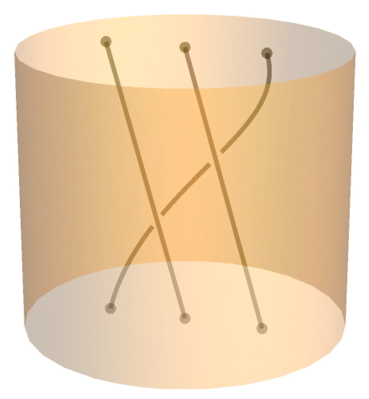
The (ordinary) fundamental group of $B(M,n)$ is the n-strand braid group of M. For the special (and much-studied Artin, or “classical“) case of $M=D^2$, we visualize elements of the n-strand braid group as collections of n monotonically descending, non-intersecting paths in $D^2\times I$ whose initial points and terminal points form the sets $\{(x_1,0),\dots ,(x_n,0)\}$ and $\{(x_1,1),\dots ,(x_n,n)\}$, respectively, where $\{x_1,\dots ,x_n\}$ is the basepoint for $B(D^2,n)$ (see Figure 7). Each path is a “strand”, which in our musical situation we may think of as a voice. It is important to keep in mind that although braid group elements are homotopy classes of paths in $B(M,n)$, due to the non-intersecting requirement, the appropriate equivalence relation for collections of paths in $D^2\times I$ representing classical braids is ambient isotopy, which closely models our physical experience with real-life braids.

It is also important to keep in mind that the space shown in pictures of braids is $D^2\times I$, not the configuration space $S{P}^n(D^2)$ itself (this is why the dimension of the visual model is the same regardless of the number of voices). A (classical) braid depicts the trace of a path of a set of n distinct points in $D^2$, with $t\in I$ corresponding to progress along the path. The group operation (concatenation) is accomplished by stacking, inverses are reflections through a horizontal plane, and the strands of identity braids are vertical line segments.

3.3.2. Singular Braids, Symmetric Products, and Orbispace Path Classes

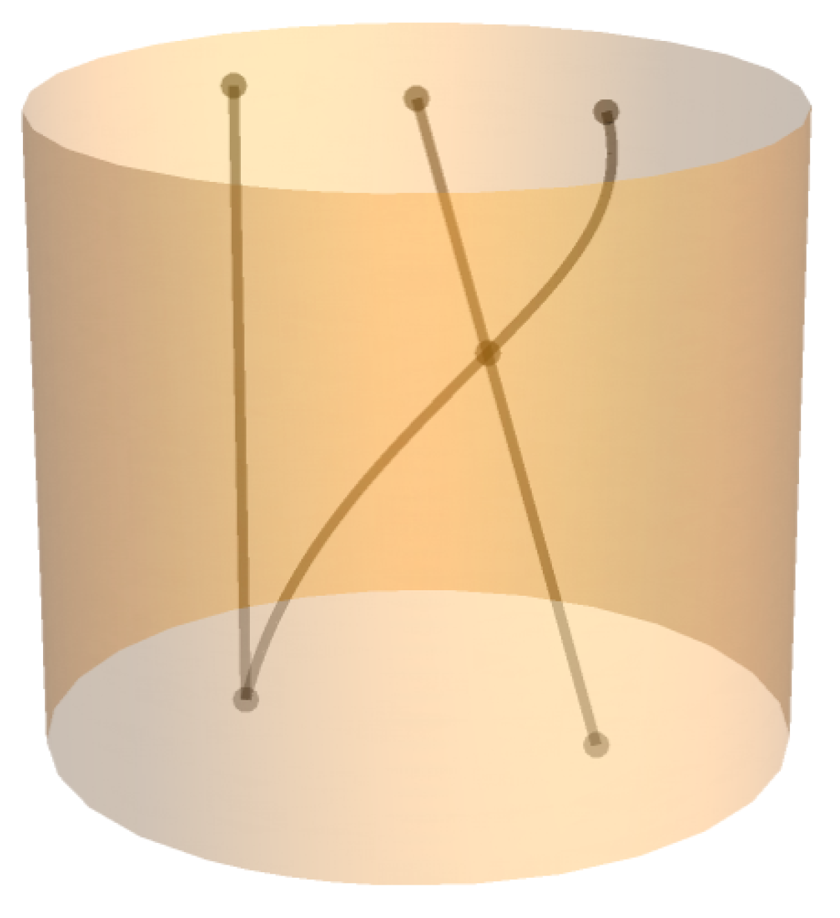
More generally, we visualize elements of the orbispace path groupoid of $S{P}^n(D^2)$ as singular braids—collections of n monotonically descending paths in $D^2\times I$ that can intersect, and whose initial and terminal point sets need not be the same subset of $D^2$ (see Figure 8).

There are two senses in which our braids are “singular”, corresponding to the two types of singularities in $S{P}^n(D^2)$. First, the paths comprising our braids can intersect with one another, and such intersections correspond to encounters of a path in $S{P}^n(D^2)$ with the singular subspace of chords with multiplicities. Second, the center point O of $D^2$ is a singularity in our context, and one or more paths in a braid passing through (or remaining on) O corresponds to an encounter of a path in $S{P}^n(D^2)$ with the singular subspace of chords with rests.

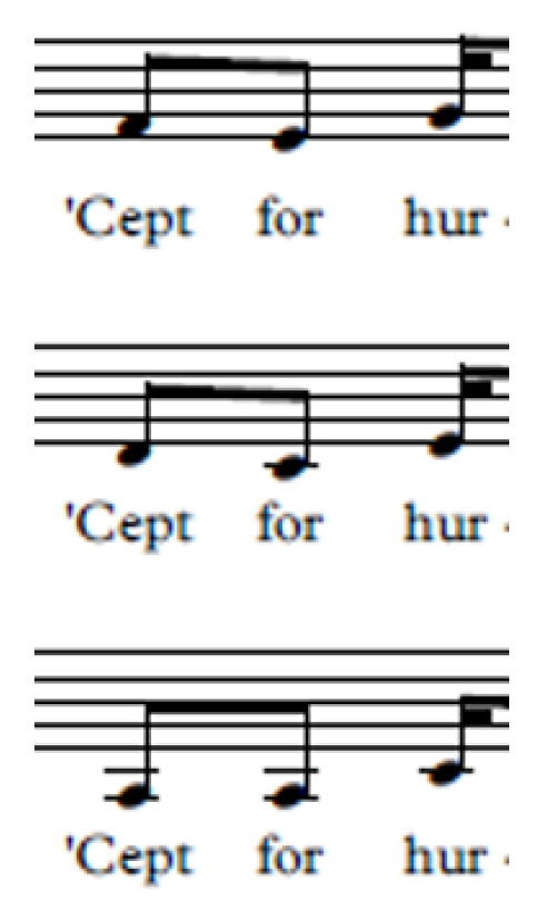
The possibility of path intersections creates a subtle but crucial way in which singular braids representing orbispace path classes differ from classical braids representing ordinary path homotopy classes. In the classical case, where strands do not intersect, a set of n non-intersecting paths is the same as a path of n-element sets. In the singular case, however, where strands can intersect, a multiset of paths is not the same as a path of multisets, because the latter does not differentiate between strands. Thus, for example, the two singular braids in Figure 9, in which the paths are distinguished by colour, represent two distinct orbispace path classes, but only one ordinary path homotopy class in $S{P}^2(D^2)$.

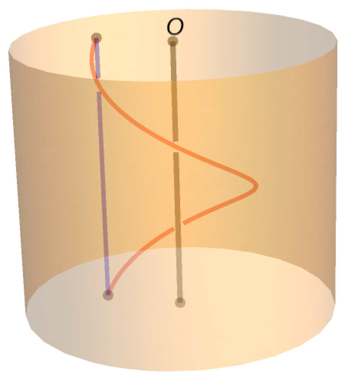
The singular role of O creates another important difference between our singular braids and classical braids. Specifically, in our orbispaces, paths that are homotopic through a homotopy that passes through O may represent distinct orbispace path classes. For example, the red and blue strands in Figure 10 are homotopic, but they represent distinct orbispace path classes. Musically, the blue strand represents a voice that remains on the same pitch (because its angular coordinate is constant), while the red strand represents a voice that ascends by an octave (because, in wrapping around the central axis of $O\times I$, its angular coordinate ascends by $2\pi$ radians). Any homotopy between the two paths must pass through $O\times I$ at least once, corresponding musically to loudness of the voice going to 0 (resting)—perhaps momentarily, but resting nonetheless.

We can think of $O\times I$ (resting) as a magic portal through which octave leaps can be accomplished without explicit annular wrapping (continuous change of pitch). Octave leaps that occur through O in this way are recorded by the element of the acting group associated with the orbispace path class. Insofar as every orbispace path class comes equipped with such an element, astute readers will note that either path in Figure 10 could “represent” either orbispace path class in the discussion; in fact, via homotopy and contact with $O\times I$, either path could represent ascent or descent by any number of octaves. As a practical matter, pictures of singular braids will be assumed not to involve such “magical” annular wrapping, but it is important to keep in mind that the possibility exists. Indeed, the definition of an orbispace path class as a path homotopy class together with a group element is what allows for the recovery of topological information lost when the circle $S^1$ is replaced by the cone on the circle $D^2$.

3.3.3. Musical Interpretations and Examples

We have already noted that each strand of a braid is musically interpretable as a voice, and that path intersections are musically interpretable as doublings. Hence, classical braids correspond to strongly crossing-free voice leadings. A strand encountering O is musically interpretable as a resting voice. We note further that voice leadings restricted to the constant-loudness subspace $r=1$ can be visualized as braids confined to the curved surface $S^1\times I$ of the cylinder $D^2\times I$. The n-strand braid group of $S^1$ is infinite cyclic (i.e., isomorphic to the additive group of integers), corresponding to the fact noted in [17] that the strongly crossing-free voice leadings of an n-note (non-singular, constant loudness) chord to itself form an infinite cyclic group. The classical (Artin) braid groups of $D^2$, corresponding to crossing-free voice leadings of chords with loudness, are considerably more complicated.

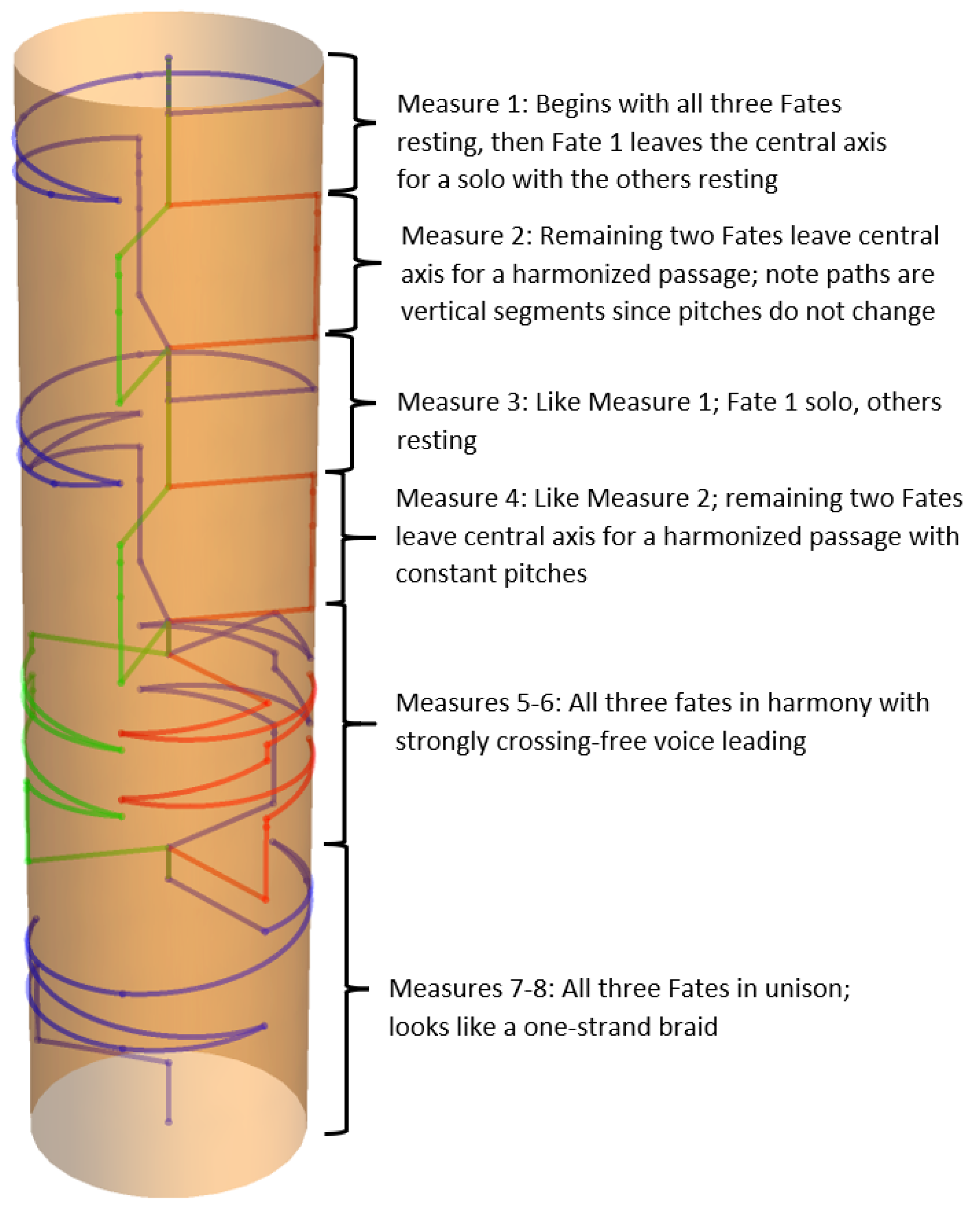
Figure 11 shows a braid rendering of the Hadestown example.

4. Discussion

There is remarkable consistency between the general model presented in this paper and modeling approaches articulated in previous work, most notably that of [5,6,16,17,19]. We have already noted how the use of orbifold paths in [6] can be extended to our model for chord space with loudness, $S{P}^n(D^2)$, which includes as a constant-loudness subspace the model for chord space $S{P}^n(S^1)$ described in [5]. In this section, we elaborate on how our model for voice leading relates to the richly detailed approach in [17].

4.1. The Paths: Basic Definitions

In [17], a path in $S^1$ (= pitch-class space) is defined to be an ordered pair $(p,r)$, where p is a point in $S^1$ (the initial point of the path) and r is a real number (the signed path length). Although the terminal point $p+r$ of the path in $S^1$ is determined by the pair $(p,r)$, Tymoczko rightly points out that the terminal point does not determine r, even if p is specified. The multitude of possible values of r for a given initial point and a given terminal point in $S^1$ corresponds to the fact that the fundamental groupoid $\pi (S^1)$ of the circle is not a tree groupoid; that is, there are multiple distinct homotopy classes of paths between any two endpoints. More specifically, what Tymoczko calls a “path in pitch-class space" actually corresponds to a homotopy class of paths in $S^1$; i.e., an element of the fundamental groupoid $\pi (S^1)$.

Tymoczko goes on to define a voice leading to be a multiset (i.e., unordered collection with multiplicities) of paths in pitch-class space, i.e., a multiset of homotopy classes of paths in $S^1$. Although he characterizes voice leadings so defined as “isomorphic to homotopy classes of paths” in the spaces $S{P}^n(S^1)$, they are actually more refined than homotopy classes of paths in $S{P}^n(S^1)$ defined in the standard way for topological spaces (since a multiset of paths conveys more information than a path of multisets). In fact, for the cases where both the initial and terminal points in $S{P}^n(S^1)$ are regular points, multisets of homotopy classes of paths in $S^1$ are in bijective correspondence with orbifold path classes in $S{P}^n(S^1)$, as we now demonstrate.

Let $\{(c_1,r_1),\dots ,(c_n,r_n)\}$ be a multiset of homotopy classes of paths in $S^1$. The multisets of initial points $\{c_1,\dots ,c_n\}$ and terminal points $\{c_1+r_1,\dots ,c_n+r_n\}$ are points in $S{P}^n(S^1)$. If we choose a particular lifting $({\tilde{x}}_1,\dots {\tilde{x}}_n)$ of $\{c_1,\dots ,c_n\}$ in the universal orbifold cover ${\mathbf{R}}^n$ (i.e., a particular basepoint in the fiber of $\{c_1,\dots ,c_n\}$ in ${\mathbf{R}}^n$; musically this is a choice of a particular assignment of the elements of $\{c_1,\dots ,c_n\}$ to voices and registers), then by the homotopy lifting properties assumed in Brown’s conditions (Section 2.2) there exists a corresponding lifting of the set of paths, and hence a lifting $({\tilde{y}}_1,\dots ,{\tilde{y}}_n)$ in the fiber (in ${\mathbf{R}}^n$) of the terminal point $\{c_1+r_1,\dots ,c_n+r_n\}$. (We can think of each ${\tilde{y}}_i$ as ${\tilde{x}}_i+r_i$, but keep mind some reordering of the $r_i$ may be needed.) If the initial and terminal points in $S{P}^n(S^1)$ are regular points, then the lifting $({\tilde{y}}_1,\dots ,{\tilde{y}}_n)$ is unique, so the mapping from voice leading to lifting of the terminal point is one to one. Conversely, given any point $({\tilde{y}}_1^{\prime },\dots ,{\tilde{y}}_n^{\prime })$ in the fiber of $\{c_1+r_1,\dots ,c_n+r_n\}$, there exists an ordered set of homotopy classes of paths in $\mathbf{R}$ with initial points ${\tilde{x}}_1,\dots {\tilde{x}}_n$ and respective terminal points ${\tilde{y}}_1^{\prime },\dots ,{\tilde{y}}_n^{\prime }$. Projecting these path classes to $S^1$ yields a multiset of path homotopy classes in $S^1$—i.e., a voice leading—whose terminal point lifts to ${\tilde{y}}_1^{\prime },\dots ,{\tilde{y}}_n^{\prime }$ when the initial point is lifted to $({\tilde{x}}_1,\dots {\tilde{x}}_n)$. Thus, the set of voice leadings between two regular points (chords) in $S{P}^n(S^1)$ is in bijective correspondence with the set of points in the fiber of the terminal point (chord) in ${\mathbf{R}}^n$. Finally, we have already observed that for given regular initial and terminal points in $S{P}^n(S^1)$, points of the fiber of the terminal point are in bijective correspondence with orbispace path classes with the given initial and terminal points, since points in the fiber of a regular point are in one-to-one correspondence with elements of the acting group.

As an example of how orbispace path classes are more refined than ordinary path homotopy classes, we note that the voice leadings $\{(C,7),(G,-7)\}$ and $\{(C,0),(G,0)\}$ are distinct according to Tymoczko’s definition (i.e., as multisets of path homotopy classes in $S^1$, and therefore as orbispace path classes), but the corresponding ordinary paths in in the topological space $S{P}^2(S^1)$ are homotopic and therefore not distinct. The topological space does not know about, and does not care about, the orbifold projection $S^1\times S^1\to S{P}^2(S^1)$, and therefore has no difficulty “homotoping the path off the boundary”. The ability of orbispace path classes to make distinctions not made by ordinary path homotopy classes is one of the main lessons of [6].

The preceding example made use of the voice leading $\{(C,7),(G,-7)\}$ which is not “strongly crossing free” in Tymoczko’s terminology. This means that there is no representative in $S^1\times S^1$ of the corresponding orbispace path class that does not have at least one point where the two voices occupy the same pitch class (a consequence of continuity and the Intermediate Value Theorem). Thus, in the chord space $S{P}^2(S^1)$, any representative of that class must encounter the boundary of the space. If we restrict paths (and homotopies thereof) to the interior of chord space (i.e., regular points), paths that encounter the boundary are disallowed, and only paths representing strongly crossing free voice leadings remain. Path classes that begin and end at the same point and do not encounter the boundary lie in a subgroup of the orbifold fundamental group that is isomorphic to the ordinary fundamental group of the space, according to a theorem of Armstrong [6]. Hence, if we restrict to the interior of $S{P}^n(S^1)$ (a manifold, and thus a space for which the ordinary fundamental group and orbifold fundamental group coincide), Tymoczko’s statement that voice leadings are isomorphic to (ordinary) homotopy classes of paths is accurate. This illustrates how musically relevant distinctions between types of voice leadings relate to distinctions between subspaces of $S{P}^n(D^2)$, and thus the importance of paying careful attention to the subspace in which we are working, since the relevant groups and groupoids can change depending on the subspace. In particular, in the case of the interior of $S{P}^n(S^1)$, the inclusion mapping into $S{P}^n(S^1)$ (or $S{P}^n(D^2)$) induces a homomorphism of the fundamental group of the interior of $S{P}^n(S^1)$ (which is isomorphic to the the additive group of integers) into the orbispace fundamental group of $S{P}^n(D^2)$, by functoriality.

If one or both of the endpoints of a voice leading (defined as a multiset of homotopy classes of paths in $S^1$) are singular points, then there will be multiple corresponding orbispace path classes, depending on the isotropy groups of the endpoints. Specifically, we have the following explanation in terms of the groupoid element assignment algorithm given in Section 2. If $\{(c_1,r_1),\dots ,(c_n,r_n)\}$ is a multiset of homotopy classes of paths in $S^1$, and the initial point $\{c_1,\dots ,c_n\}$ is singular, then it will have non-trivial isotropy group; hence there will be multiple choices for a group element ${\gamma }_0$ taking a given lifting $({\tilde{x}}_1,\dots ,{\tilde{x}}_n)$ of $\{c_1,\dots ,c_n\}$ into a preferred fundamental domain, and therefore multiple choices for $\gamma$ taking the lifting ${\gamma }_0·({\tilde{x}}_1+r_1,\dots ,{\tilde{x}}_n+r_n)$ of the terminal point into a preferred fundamental domain. Likewise, if the terminal point $\{c_1+r_1,\dots ,c_n+r_n\}$ is singular, then it will have non-trivial isotropy group, so there will be multiple choices for $\gamma$ in that case as well.

Tymoczko notes in the appendix of [17] that the distinctions among multiple orbispace path classes corresponding to a single multiset of homotopy classes of paths in $S^1$ are potentially “unobservable” if one looks only at the endpoints. As noted in Section 2, the distinctions become observable in the presence of intervening points; i.e., by parsing a voice leading into a concatenation of voice leadings. For example, the distinction between the two orbispace path classes $(\{A,A\},\{A,A\},\left(\begin{array}{cc}1& 2\\ 1& 2\end{array}\right))$ and $(\{A,A\},\{A,A\},\left(\begin{array}{cc}1& 2\\ 2& 1\end{array}\right))$ corresponding to the voice leading $\{(A,0),(A,0)\}$ becomes observable if the voice leading is parsed as $\{(A,2),(A,-2)\}$ followed by $\{(B,-2),(G,2)\}$. Again, it is important to note that paths corresponding to such a parsing exist even in the homotopy class of the constant path from $(A,A)$ to itself, unless the ambient space is restricted to the subspace $C_1^2$ of two-voice unisons. (Tymoczko implicitly imposes such a restriction in his discussion; this again illustrates the importance of specifying the ambient subspace.)

The preceding discussion presupposes a concatenation operation on voice leadings. Tymoczko does not give a formal definition of voice leading concatenation in the main body of [17], but the following definition appears in the appendix: “A concatenation of two voice leadings $v_1$ and $v_2$ is a bijection between their paths such that each path in $v_1$ is connected to its partner in $v_2$”. We render this definition in mathematical terms as follows. Two voice leadings $v_1=\{(c_1,r_1),\dots ,(c_n,r_n)\}$ and $v_2=\{(d_1,s_1),\dots ,(d_n,s_n)\}$ can be concatenated (in the given order) if and only if $\{d_1,\dots ,d_n\}=\{c_1+r_1,\dots ,c_n+r_n\}$, and if that is the case and we reorder the elements so that $c_i+r_i=d_i$ for $i=1,\dots ,n$, then the concatenation of the two voice leadings is $\{(c_1,r_1+s_1),\dots ,(c_n,r_n+s_n)\}$. We note that the required reordering of elements is the “bijection” to which Tymoczko refers, and the equations $c_i+r_i=d_i$ refer to the phrase “connected to its partner”. Tymoczko also makes use of inverse (“retrograde”) voice leadings, implicitly defining the inverse of $\{(c_1,r_1),\dots ,(c_n,r_n)\}$ to be $\{(c_1+r_1,-r_1),\dots ,(c_n+r_n,-r_n)\}$.

We now show that for voice leadings between regular points, Tymoczko’s definitions of concatenation and inverses agree with the corresponding definitions given above for orbispace path classes. Let $\{(c_1,r_1),\dots ,(c_n,r_n)\}$ and $\{(d_1,s_1),\dots ,(d_n,s_n)\}$ be two voice leadings for which concatenation in the given order is possible. Let a preferred fundamental domain in ${\mathbf{R}}^n$ be specified, and let $({\tilde{c}}_1,\dots ,{\tilde{c}}_n)$ be the unique representative of $\{c_1,\dots ,c_n\}$ in that fundamental domain. Note that this representative is an ordered set, and ${\tilde{c}}_i$ may not correspond to $c_i$ (i.e., some reordering may be needed). Nevertheless, since $\{c_1,\dots ,c_n\}$ is a regular point, we can apply the same reordering to the $r_i$ without ambiguity, so without loss of generality we can assume $({\tilde{c}}_1+r_1,\dots ,{\tilde{c}}_n+r_n)$ is the terminal point of a path in ${\mathbf{R}}^n$ corresponding to the first voice leading. Since $\{d_1,\dots ,d_n\}$ is a regular point, there is a unique element $\gamma$ of ${\mathbf{Z}}^n⋊{\Sigma }_n$ that takes $({\tilde{c}}_1+r_1,\dots ,{\tilde{c}}_n+r_n)$ into the preferred fundamental domain. Thus, the first voice leading corresponds to the element $(\{c_1,\dots ,c_n\},\{c_1+r_1,\dots ,c_n+r_n\},\gamma )$ of the orbifold path groupoid. Similarly, the second voice leading corresponds to the element $(\{d_1,\dots ,d_n\},\{d_1+s_1,\dots ,d_n+s_n\},\delta )$, where $\delta$ is the unique element of of ${\mathbf{Z}}^n⋊{\Sigma }_n$ that takes $({\tilde{d}}_1+s_1,\dots ,{\tilde{d}}_n+s_n)$ into the preferred fundamental domain, and $({\tilde{d}}_1,\dots ,{\tilde{d}}_n)$ is the unique representative of $\{d_1,\dots ,d_n\}$ in the preferred fundamental domain. Note that since $\{c_1+r_1,\dots ,c_n+r_n\}=\{d_1,\dots ,d_n\}$, $\gamma ·({\tilde{c}}_1+r_1,\dots ,{\tilde{c}}_n+r_n)$ must coincide with $({\tilde{d}}_1,\dots ,{\tilde{d}}_n)$. Now, the concatenation of the two voice leadings is given above as $\{(c_1,r_1+s_1),\dots ,(c_n,r_n+s_n)$, but the notation includes an assumption that the $s_i$ have been reordered according to the stipulation that each $c_i+r_i=d_i$. Hence, a path in ${\mathbf{R}}^n$ from $({\tilde{c}}_1,\dots ,{\tilde{c}}_n)$ to $({\tilde{c}}_1+r_1+s_1,\dots ,{\tilde{c}}_n+r_n+s_n)$ is homotopic to the concatenation of paths from $({\tilde{c}}_1,\dots ,{\tilde{c}}_n)$ to $({\tilde{c}}_1+r_1,\dots ,{\tilde{c}}_n+r_n)$ and from ${\gamma }^{-1}·({\tilde{d}}_1,\dots ,{\tilde{d}}_n)$ to ${\gamma }^{-1}·({\tilde{d}}_1+s_1,\cdots ,{\tilde{d}}_n+s_n)$. The terminal points must coincide, so the unique member of ${\mathbf{Z}}^n⋊{\Sigma }_n$ taking $({\tilde{c}}_1+r_1+s_1,\dots ,{\tilde{c}}_n+r_n+s_n)$ into the preferred fundamental domain must be $\delta \gamma$, which means the voice leading $\{(c_1,r_1+s_1),\dots ,(c_n,r_n+s_n)\}$ corresponds to the element $(\{c_1,\dots ,c_n\},\{d_1+s_1,\dots ,d_n+s_n\},\delta \gamma )$ of the orbispace path groupoid, i.e., the concatenation of the groupoid elements $(\{c_1,\dots ,c_n\},\{c_1+r_1,\dots ,c_n+r_n\},\gamma )$ and $(\{d_1,\dots ,d_n\},\{d_1+s_1,\dots ,d_n+s_n\},\delta )$. The argument for inverses is similar, and we omit it for brevity.

If any of the endpoints of voice leadings to be concatenated (specified as multisets of homotopy classes of paths in $S^1$) are singular, then there is ambiguity in the orbispace path classes involved, as explained above. Hence, we expect ambiguity in both the process and the result of concatenation. However, Tymoczko’s definition astutely provides a way to resolve ambiguity at the intermediate point of concatenation by requiring specification of a particular bijection between the multisets of paths, so that the ambiguity of the result is no different than the ambiguity that would arise from singularity of the endpoints of the concatenation. We illustrate with two examples.

First, consider the two voice leadings $\{(G,2),(B,-2)\}$ and $\{(A,-2),(A,2)\}$. Concatenation in the given order is possible, and the endpoints of the concatenation once performed will both be regular. On the other hand, the intermediate point $\{A,A\}$ is singular. Hence, there are two elements of the orbispace path groupoid corresponding to the first voice leading, namely $(\{G,B\},\{A,A\},\left(\begin{array}{cc}1& 2\\ 1& 2\end{array}\right))$ and $(\{G,B\},\{A,A\},\left(\begin{array}{cc}1& 2\\ 2& 1\end{array}\right))$. Likewise there are two elements corresponding to the second voice leading, $(\{A,A\},\{G,B\},\left(\begin{array}{cc}1& 2\\ 1& 2\end{array}\right))$ and $(\{A,A\},\{G,B\},\left(\begin{array}{cc}1& 2\\ 2& 1\end{array}\right))$. Thus, the concatenation of the two voice leadings can be either $(\{G,B\},\{G,B\},\left(\begin{array}{cc}1& 2\\ 1& 2\end{array}\right))$ or $(\{G,B\},\{G,B\},\left(\begin{array}{cc}1& 2\\ 2& 1\end{array}\right))$. If the voice leadings are specified as groupoid elements at the outset, then their concatenation is determined unambiguously by the concatenation operation in the groupoid. If, on the other hand, the voice leadings are specified as multisets of paths, then to concatenate them requires specification of a bijection from $\{(G,2),(B,-2)\}$ to $\{(A,2),(A,-2)\}$; once it is specified the concatenation is determined to be either $\{(G,0),(B,0)\}$ or $\{(G,4),(B,-4)\}$. Thus, in either setting, we obtain an unambiguous result; the difference lies in whether the ambiguity is resolved at the level of individual voice leadings, or at the level of concatenations of voice leadings.

For our second example, consider the voice leadings $\{(A,2),(A,-2)\}$ and $\{(G,2),$$(B,-2)\}$. In this case, the intermediate point is regular, but the endpoints are singular. For each voice leading, there are two possible corresponding groupoid elements, but there is only one choice for a bijection between the paths fulfills the “connected” condition. Hence, some ambiguity of groupoid element remains after concatenation according to Tymoczko’s definition, but it is the same ambiguity that would be present for the concatenated voice leading $\{(A,0),(A,0)\}$ in any case.

Tymoczko uses the term “contrapuntal design” for a sequence of concatenations. Specifically, for an n-voice, m-chord passage, he defines a contrapuntal design to be “a multiset of m-tuples whose elements form a sequence of paths in pitch-class space, each connected to its successor, with each m-tuple representing a distinct melodic line”. Let

$$\{((c_{1,1},r_{1,1}),\dots ,(c_{1,m},r_{1,m})),\dots ,((c_{n,1},r_{n,1}),\dots ,(c_{n,m},r_{n,m}))\}$$

be such a multiset of n sequences of m paths. Then

$$(\{(c_{1,1},r_{1,1}),\dots ,(c_{n,1},r_{n,1})\},\dots ,\{(c_{1,m},r_{1,m}),\dots ,(c_{n,m},r_{n,m})\})$$

is a sequence of voice leadings, with specific bijections for concatenating adjacent voice leadings encoded in the first subscript (i.e., for $1\le i\le n$ and $1\le j\le m-1$, the path $(c_{i,j}$ is to be “partnered with” $c_{i,j+1}$). Thus, a contrapuntal design uniquely determines a sequence of concatenations of voices leadings. Likewise a sequence of concatenations uniquely determines a contrapuntal design, so the two terms are essentially synonymous. If all the chords involved are regular points, a contrapuntal design is the same as a sequence of concatenated elements of the orbispace path groupoid (i.e., a factorization or word in the elements of the groupoid). If singular points are involved, then multiple factorizations in the groupoid will correspond to a single contrapuntal design, for reasons discussed above.

4.2. The Subspaces: Relevant Restrictions

We have already noted that the chord spaces considered in [17] are constant-loudness subspaces of our generalized chord spaces $C^n=S{P}^n(D^2)$, and within these subspaces, chords without doublings are subspaces consisting of regular points. Here, we discuss some other musically relevant restrictions and inclusions.

A common phenomenon in music is persistent, specified voice doublings throughout a passage. Such passages can be regarded as restrictions to a subspace $C_{k,k}^n$ of $C^n$ consisting of n voices on exactly k parts. The orbispace path groupoid of such a subspace is isomorphic to that of k-voice space. In particular, for the special case $k=1$ (all voices in unison), as long as the restriction persists (i.e., no voice is allowed to stray from the unison), the orbispace path groupoid is isomorphic to $T(S^1)⋊\mathbf{Z}$. The absence of a symmetric group factor in this situation removes the redundancy of multiple groupoid elements associated with “unobservable” voice exchanges discussed in the appendix of [17].

A generalization of persistent, specified voice doublings is a persistent, specified interval between specified voices. This phenomenon is discussed at length in [19]. Chords and voice leadings subject to such constraints are restricted to appropriately defined subspaces of $C^n$, analogous to $C_{k,k}^n$.

Another common phenomenon is specified resting voices throughout a passage. An n-voice passage with $n-k$ resting voices resides in the subspace of $C^n$ identified with $C^k$ as described in Section 3. If we further specify that the k non-resting voices have equal and constant loudness, then we can regard the subspace as $S{P}^k(S^1)$; its inclusion into $C^n$ induces a morphism of orbispace path groupoids, by functoriality. Such inclusions of subspaces with resting voices provide a way to combine chords of different cardinalities, an endeavor deemed problematic in Section 2 of [17] and in [7].

4.3. Moves of Musical Interest

Tymoczko identifies several types of voice leading moves that are of musical interest, not only because they occur frequently in actual music, but also because they comprise a relatively small collection of moves (math: generators) in terms of which much larger collections can be described. These types of moves are stepwise transpositions along the chord (denoted by $t_i$ in [17]), transpositions along the scale (denoted by $T_j$), basic voice leadings, and diagonal actions. In this subsection, we provide interpretations of these moves in terms of the orbispace path groupoid.

Given an n-note (non-singular) chord, the stepwise transposition along the chord $t_i$ applies a cyclic permutation to the pitch classes of the chord. Defining and interpreting $t_i$ as a voice leading, however, require more precision, since a path representing the permutation may incur changes in register. Specifically, $t_1$ moves each note upward to the next note of the chord, so the highest note will be moved to a different fundamental domain. Assuming constant loudness and taking as preferred fundamental domain the set of representatives that satisfy $C4\le x_1<x_2<\cdots <x_n<C5$ for each chord $\{x_1,\dots ,x_n\}$, $t_1$ takes $(x_1,\dots ,x_n)$ to $(x_2,x_3,\dots ,x_n,x_1+\mathbf{o})$ (where $\mathbf{o}$ denotes the size of the octave). The element of the acting group that moves $(x_2,x_3,\dots ,x_n,x_1+\mathbf{o})$ to its unique representative in the preferred fundamental domain is

$$(-1,0,\dots ,0)\circ \left(\begin{array}{ccccc}1& 2& \dots & n-1& n\\ 2& 3& \dots & n& 1\end{array}\right)$$

and the corresponding forward-moving element is its inverse

$$(0,\dots ,0,1)\circ \left(\begin{array}{ccccc}1& 2& \dots & n-1& n\\ n& 1& \dots & n-2& n-1\end{array}\right).$$

(The initial and terminal chords are the same, so we do not notate them explicitly here.) We obtain group elements corresponding to the other $t_i$ by taking appropriate powers of these elements. In particular, we note that the forward-moving element corresponding to $t_n$ is $(1,1,\dots ,1)\circ 1$, which raises each note by an octave.

Transposition along the scale requires specification of a scale, defined as follows in the appendix of [17]:

“A scale is a collection of $\mathbf{o}$ distinct pitch classes defining a piecewise linear metric with the distance between adjacent notes equal to one (‘the scale step’); we use this metric to label pitch classes with integers, choosing an arbitrary element as pitch class 0 and proceeding in the ascending direction”.

From the context of this definition, we infer that $\mathbf{o}$ is to be a positive integer, and a scale is an ordered set $(d_1,\dots ,d_{\mathbf{o}})$ of elements of $S^1$, with the ordering compatible with angles assigned to elements of $S^1$. As an operation on the entire scale, transposition along the scale is no different from transposition along a chord, so the element of the acting group corresponding to $T_1$ is

$$(0,\dots ,0,1)\circ \left(\begin{array}{ccccc}1& 2& \dots & \mathbf{o}-1& \mathbf{o}\\ \mathbf{o}& 1& \dots & \mathbf{o}-2& \mathbf{o}-1\end{array}\right)$$

with powers of this element corresponding to the other $T_j$.

Typically, though, transposition $T_j$ along a specified scale $(d_1,\dots ,d_{\mathbf{o}})$ will be applied to a chord $\{d_{k_1},\dots ,d_{k_n}\}$ consisting of $n<\mathbf{o}$ distinct pitch classes drawn from the scale, and the corresponding group element will be the restriction of the above transformation to this subset. Such a restriction will typically change the chord, so we include the initial and terminal chords in the notation of the corresponding groupoid element. We specify a preferred fundamental domain by requiring the representative therein, $({\tilde{x}}_1,\dots ,{\tilde{x}}_n)$, of a (non-singular, constant loudness) n-note chord $\{x_1,\dots ,x_n\}$ to satisfy ${\tilde{d}}_1\le {\tilde{x}}_1<{\tilde{x}}_2<\dots <{\tilde{x}}_n<{\tilde{d}}_1+\mathbf{o}$, where ${\tilde{d}}_1$ is any fixed pitch in the pitch class $d_1$. We then assume $({\tilde{d}}_{k_1},\dots ,{\tilde{d}}_{k_n})$ is such a representative of our starting chord (i.e., the initial point of a representative path for the voice leading). The terminal point of the corresponding path representing $T_1$ will then be $({\tilde{d}}_{k_1+1},\dots ,{\tilde{d}}_{k_n+1})$ if $k_n<\mathbf{o}$, and $({\tilde{d}}_{k_1+1},\dots ,{\tilde{d}}_1+\mathbf{o})$ if $k_n=\mathbf{o}$. Thus, the groupoid element corresponding to $T_1$ is $(\{d_{k_1},\dots ,d_{k_n}\},\{d_{k_1+1},\cdots ,d_{k_n+1(mod\mathbf{o})}\},\sigma )$, where the permutation $\sigma$ is the identity if $k_n<\mathbf{o}$, and $(-1,0,\dots ,0)\circ \left(\begin{array}{cccc}1& 2& \dots & n\\ 2& 3& \dots & 1\end{array}\right)$ if $k_n=0$. The contingencies become more complicated for the other $T_j$; in such cases, ad hoc computation is preferable to general formulas.

Tymoczko defines a basic voice leading in [17] as combining $t_{-1}$ with $T_2$, in the case of 3-note chords in a 7-note scale (basic voice leadings in other contexts would presumably involve different subscripts). For example, a basic voice leading applied to a C major chord in a C major scale would take (C4, E4, G4) first to (G3, C4, E4) and then to (B3, E4, G4). The groupoid element corresponding to this voice leading is $(\{C,E,G\},\{B,E,G\},(0,0,1)\circ \left(\begin{array}{ccc}1& 2& 3\\ 3& 1& 2\end{array}\right))$. On the other hand, a basic voice leading applied to (E4, G4, B4) has corresponding groupoid element $(\{E,G,B\},\{D,G,B\},1)$. The associated group element is the identity in this case because of register and fundamental domain considerations, but in all cases a basic voice leading changes exactly one pitch class of the chord, and applies a (possibly trivial) cyclic permutation, possibly with a single register change.

In [17], a diagonal action is similar to a basic voice leading, except that it applies to 3-note chords in a 12-note scale, and $t_{-1}$ is combined with $T_4$ instead of $T_2$. One example Tymoczko gives is (C4, E4, G4) to (B3, E4, G♯4), which has corresponding groupoid element $(\{C,E,G\},\{B,E,G♯\},(0,0,1)\circ \left(\begin{array}{ccc}1& 2& 3\\ 3& 1& 2\end{array}\right))$. Another example takes (C4, F4, G4) to (B3, E4, A4) with corresponding groupoid element $(\{C,F,G\},\{B,E,A\},(0,0,1)\circ \left(\begin{array}{ccc}1& 2& 3\\ 3& 1& 2\end{array}\right))$. It is interesting to note that the associated element of the acting group is the same for the two examples, and for first basic voice leading example given above.

4.4. Transpositional and Inversional Set-Class Spaces

Transpositional and inversional set-class spaces are quotient spaces resulting from the imposition of additional musically relevant equivalences on chord spaces. Sections 3 and 4 of [17] provide a wealth of detail pertaining to voice leading in these spaces. Insofar as the formalism of orbispace path classes and orbispace path groupoids can be applied equally well to any of the quotient spaces, we will confine ourselves here to a brief discussion of fundamental domains and acting groups for the transpositional case, and finding orbispace path groupoid elements for one example.

Transpositional set-class space is chord space modulo uniform transposition of chords. The geometrical normal form conditions NF1–NF3 given in [17] and repeated below define a preferred fundamental domain. An n-tuple of pitches $(x_0,x_1,\dots ,x_{n-1})$ is in geometrical normal form if

NF1.

Its first element is 0;

NF2.

It is in ascending order, with the final element less than or equal to the octave $\mathbf{o}$;

NF3.

Its smallest interval lies between its first two notes (including the “wraparound” interval $\mathbf{o}-x_{n-1}$ among the chord’s intervals).

The acting group is ${\mathbf{Z}}_n⋊({\mathbf{Z}}^{n-1}⋊{\Sigma }_n)$. Uniform transposition is used to obtain NF1. For NF2, the action of ${\Sigma }_n$ is used to arrange pitches in ascending order, and the action of ${\mathbf{Z}}^{n-1}$ is used to bring all pitches within a single octave (only $n-1$ factors are needed because of NF1). Finally, the action of the cyclic group ${\mathbf{Z}}_n$ is used (along with additional octave adjustments) to obtain NF3 (and preserve NF2). The procedure for associating a groupoid element with a voice leading is the same as given earlier for chord spaces: uniformly transform the voice leading so that the initial point is in the preferred fundamental domain, then find an element of the acting group that moves the transformed terminal point into the preferred fundamental domain.

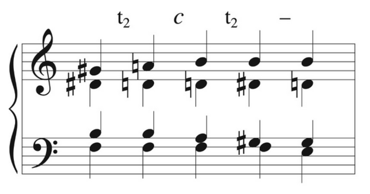
Applying the procedure to the sequence of voice leadings in Figure 27 of [17] (Figure 12), we obtain the groupoid element

$$((0258),(0258),2_4\circ (0,-1,-1)\circ 1)$$

for both voice leadings labeled $t_2$ in the figure (where $2_4$ denotes the congruence class of 2 in ${\mathbf{Z}}_4$, and $(0258)$ denotes the set class which is unchanged in these voice leadings), and

$$(0258),(0258),1_4\circ (0,0,0)\circ \left(\begin{array}{cccc}1& 2& 3& 4\\ 2& 1& 3& 4\end{array}\right)$$

for the the voice leading labeled c. The last voice leading connects different set classes; its associated groupoid element is $((0258),(0269),1)$, the group element of which is the identity since the terminal point is already in the preferred fundamental domain.

Obtaining groupoid interpretations of voice leadings in the case of inversional set-class spaces works similarly, with appropriate changes to the fundamental domains and acting groups. For brevity, we defer this intriguing task to later work.

5. Conclusions

On page 134 of [17], the following statement appears: “... we can interpret the geometrical pattern of boundary interactions as a sequence of abstract transformations combining to produce the total voice leading”. In many ways, this statement summarizes and encapsulates the relationships between orbispaces, orbispace path classes, and voice leading. To begin, a “boundary interaction” refers to a path in a fundamental domain for an orbispace $p:X\to X/G$ that intersects the boundary of that fundamental domain. Such a fundamental domain lies in X, which we take to be the universal orbispace cover. Importantly, the space X is partitioned into (“tiled by”) copies of the fundamental domain, and boundary encounters are necessary for passage from one fundamental domain into another. Insofar as the copies of the fundamental domain correspond by definition to elements of the acting group G, the correspondence between boundary interactions and “abstract transformations” (i.e., elements of G) is mathematically precise (see Figure 2 for illustration). The definition of orbispace path class captures the precise mathematical correspondence between boundary encounters that occur when traveling from one fundamental domain to another. (Interestingly, these ideas are broadly reminiscent of Vassiliev’s approach to knot theory 30 years ago.)

Since the universal orbispace cover X is simply connected, any two paths in X from a given initial point to a given terminal point are homotopic. The variability in paths within a homotopy class corresponds to variability in factorizations of a given orbispace path class. In Section 5 of [17], Tymoczko characterizes such factorizations as “words” in the “alphabet” of transformations, and in so doing invokes the broad topic of word theory, used extensively in [20] and elsewhere in mathematical music theory. One of the main goals of this paper is to clarify the isomorphism—deemed “challenging” in [17]—between the “alphabet” of transformations and the acting group G of symmetries. Their essential identity lies at the heart of geometric and topological modeling of voice leading.

References

- Mitchell, A.; Chavkin, R.; Carney, R.; DeShields, A.; Gray, A.; Noblezada, E.; Page, P.; Robinson, L. Hadestown: Original Broadway Cast Recording; Sing It Again: New York, NY, USA, 2019. [Google Scholar]
- Lewin, D. Some Ideas About Voice-leading Between PCsets. J. Music Theory 1998, 42, 15–72. [Google Scholar] [CrossRef]
- Roeder, J. A geometric representation of pitch-class series. Perspect. New Music 1987, 25, 362–409. [Google Scholar]
- Callender, C. Continuous Transformations. Music Theory Online 2004, 10, 3. [Google Scholar]
- Callender, C.; Quinn, I.; Tymoczko, D. Generalized voice-leading spaces. Science 2008, 320, 346–348. [Google Scholar] [CrossRef] [PubMed] [Green Version]
- Hughes, J. Using Fundamental Groups and Groupoids of Chord Spaces to Model Voice Leading. In Mathematics and Computation in Music, Proceedings of the 5th International Conference; Collins, T., Meredith, D., Volk, A., Eds.; Lecture Notes in Artificial Intelligence; Springer: Heidelberg, Germany, 2015; Volume 9110, pp. 267–278. [Google Scholar]
- Genuys, G. Pseudo-distances between chords of different cardinality on generalized voice-leading spaces. J. Math. Music 2019, 13, 193–206. [Google Scholar] [CrossRef]
- Arias-Valero, J.S.; Lluis-Puebla, E. Some remarks on hypergestural homology of spaces and its relation to classical homology. J. Math. Music 2020, 14, 245–265. [Google Scholar] [CrossRef]
- Mannone, M. Knots, Music and DNA. J. Creat. Music Syst. 2018, 2, 3–12. [Google Scholar] [CrossRef] [Green Version]
- Mazzola, G. The Topos of Music; Birkhauser: Basel, Switzerland, 2002; p. 1335. [Google Scholar]
- Jedrzejewski, F. Hétérotopies Musicales: Modèles Mathématiques de la Musique; Hermann: Paris, France, 2019; p. 670. [Google Scholar]
- Xenakis, I. Formalized Music: Thought and Mathematics in Composition; Pendradon Press: Sheffield, MA, USA, 1992; p. 400. [Google Scholar]
- Morton, H. Symmetric Products of the Circle. Math. Proc. Camb. Philos. Soc. 1967, 63, 349–352. [Google Scholar] [CrossRef]
- Brown, R. Topology and Groupoids; Booksurge: Deganwy, UK, 2006; p. xxvi+512. [Google Scholar]
- Dragomir, G. Closed Geodesics on Orbifolds. Ph.D. Thesis, McMaster University, Hamilton, ON, Canada, 2011. [Google Scholar]
- Tymoczko, D. A Geometry of Music: Harmony and Counterpoint in the Extended Common Practice; Oxford University Press: Oxford, UK, 2011; p. 480. [Google Scholar]
- Tymoczko, D. Why topology? J. Math. Music 2020, 14, 114–169. [Google Scholar] [CrossRef]
- Kallel, S. Symmetric products, duality and homological dimension of configuration spaces. Geom. Topol. Monogr. 2008, 13, 499–527. [Google Scholar]
- Bulger, D.; Cohn, R. Constrained voice-leading spaces. J. Math. Music 2016, 10, 1–17. [Google Scholar] [CrossRef]
- Clampitt, D.; Noll, T. Naming and ordering the modes, in light of combinatorics on words. J. Math. Music 2019, 12, 134–153. [Google Scholar] [CrossRef]
Figure 1.
Author’s transcription of an excerpt from “Any Way the Wind Blows” from Hadestown showing the use of solos with resting voices, harmonized voices, and unison voices in quick succession. In some Broadway performances, the solo in the third measure is taken by Fate 2. The orbifold path model can distinguish the two different assignments.
Figure 2.
A visual representation of the paths involved in the proof of Theorem 2.
Figure 3.
A schematic illustration of the process by which a groupoid element is associated with a voice leading. Diamond-shaped regions depict fundamental domains in the universal orbispace cover X; green shading indicates the preferred fundamental domain. Solid blue curves are paths; dashed orange lines represent group actions.
Figure 4.
The first three chords of the fifth measure of the Hadestown excerpt; all voices treble clef.
Figure 5.
An excerpt from an unpublished work by R. Joseph Lubben.
Figure 6.
Illustration of proof of Theorem 4.
Figure 7.
A classical 3-strand braid.
Figure 8.
A singular 3-strand braid.
Figure 9.
Two different orbispace paths corresponding to the same singular braid.
Figure 10.
The paths are homotopic, but only through a homotopy that encounters .
Figure 11.
The Hadestown example as a singular braid. The blue strand is Fate 1, the red strand is Fate 2, and the green strand is Fate 3. Resting voices are on the central axis; sounding voices are on the curved outer surface.
Figure 12.
Figure 27 from [17].
Publisher’s Note: MDPI stays neutral with regard to jurisdictional claims in published maps and institutional affiliations. |
© 2022 by the author. Licensee MDPI, Basel, Switzerland. This article is an open access article distributed under the terms and conditions of the Creative Commons Attribution (CC BY) license (https://creativecommons.org/licenses/by/4.0/).
Share and Cite
MDPI and ACS Style
Hughes, J.R. Generalizing the Orbifold Model for Voice Leading. Mathematics 2022, 10, 939. https://doi.org/10.3390/math10060939
AMA Style
Hughes JR. Generalizing the Orbifold Model for Voice Leading. Mathematics. 2022; 10(6):939. https://doi.org/10.3390/math10060939
Chicago/Turabian StyleHughes, James R. 2022. "Generalizing the Orbifold Model for Voice Leading" Mathematics 10, no. 6: 939. https://doi.org/10.3390/math10060939
Note that from the first issue of 2016, this journal uses article numbers instead of page numbers. See further details here.