Evaluation of sEMG Signal Features and Segmentation Parameters for Limb Movement Prediction Using a Feedforward Neural Network

Abstract

Limb movement prediction based on surface electromyography (sEMG) for the control of wearable robots, such as active orthoses and exoskeletons, is a promising approach since it provides an intuitive control interface for the user. Further, sEMG signals contain early information about the onset and course of limb movements for feedback control. Recent studies have proposed machine learning-based modeling approaches for limb movement prediction using sEMG signals, which do not necessarily require domain knowledge of the underlying physiological system and its parameters. However, there is limited information on which features of the measured sEMG signals provide the best prediction accuracy of machine learning models trained with these data. In this work, the accuracy of elbow joint movement prediction based on sEMG data using a simple feedforward neural network after training with different single- and multi-feature sets and data segmentation parameters was compared. It was shown that certain combinations of time-domain and frequency-domain features, as well as segmentation parameters of sEMG data, improve the prediction accuracy of the neural network as compared to the use of a standard feature set from the literature.

1. Introduction

Wearable robots, such as active orthoses or exoskeletons, gain importance in rehabilitation as aids for people with disabilities, e.g., those induced by neuromuscular disorders, or in the support of people during physical labour [1,2,3,4]. Whereas passive orthoses, such as spring-loaded systems [5,6,7], provide immediate but uncontrolled support, current active (i.e., motorized) systems based on force or torque sensors [8] provide a controlled but unintuitive, delayed reaction of the technical system. The model-based prediction of limb movements based on surface electromyography (sEMG) is a basis for more intuitive control of active orthoses as neural signals that induce muscle contractions precede the actual limb movement. These signals can, therefore, be used to predict the behavior of the musculoskeletal apparatus before actual movements take place. However, sEMG signals vary strongly between subjects, for example, due to differences in body composition or electrode placement. Additionally, mere muscle contractions can lead to measurement inaccuracies, as the electrodes shift on the skin during muscle movement [9,10,11]. Therefore, to predict limb movement from sEMG signals and control active body support systems, an adaptive model with the ability to compensate for inter-subject variations and motion artifacts would be desirable. sEMG-based prediction models are classically based on Hill-type muscle models [12], which represent the contraction dynamics of the muscle based on various physiological parameters. The activation of the muscle based on neural signals (measured as sEMG signals) is usually modeled by the so-called activation dynamics, i.e., the electrochemical conversion of neuronal excitation into the release of Ca²⁺ ions into the muscle sarcomeres [13,14]. As an alternative to classical models, such as Hill’s muscle model, machine learning offers the potential to capture the complexity of neurally controlled muscle contraction without the need for domain knowledge of the underlying biomechanical properties and physiological relationships. Since machine learning models are purely data driven and do not rely on physiological parameters that, for example, have to be determined experimentally (as in approaches requiring domain knowledge), they can be easily adapted to inter-subject variations using, for example, transfer learning [15]. Several studies have been performed on the classification or prediction of limb movements using machine learning models. A backpropagation neural network was used by [16] to estimate upper limb joint angles. In [17], a neurofuzzy matrix modifier was applied to create an adaptive upper limb controller. Support vector regression was proposed in [18] to estimate wrist movements in real time. In [19], various EMG features and feature segmentations were investigated for support-vector-machine-based movement classification for upper limb myoelectric control. Different EMG pattern recognition methods and EMG features were compared in [20]. A deep neural network was used to classify wrist positions in [21]. EMG signal quality estimates were also examined in [22]. While a majority of studies have focused on machine learning model architectures for sEMG-based limb movement prediction, studies on the corresponding feature selection and segmentation of sEMG signals are scarce. In the work presented here, an overview-like review of sEMG features and segmentation parameters appropriate for elbow motion prediction based on neural networks is given. Therefore, different single- and multi-feature sets and segmentation parameters of sEMG signals are systematically investigated and compared with respect to the performance of limb movement prediction, using a simple feedforward neural network (FFNN). By choosing the simplest version of an FFNN architecture restricted to only one hidden layer, the prediction quality should depend on the signal features and segmentation parameters rather than the complexity of the underlying network architecture. Thus, the procedure for feature and segmentation parameter extraction as well as the results presented have the potential to be extrapolated to more complex neural network architectures. To investigate the signal features and segmentation parameters, sEMG data from four muscle heads of the human upper arm and the corresponding elbow joint angle were recorded while subjects performed various movement sequences requiring activation of said muscle groups. Afterwards, features were selected from different categories based on the experimentally collected sEMG data. Within sEMG signal segments of different lengths, these features were extracted and used for training the FFNN to predict the associated elbow joint movement of the upper arm. The accuracy of the trained FFNN based on the feature categories and different segmentation parameters applied to the sEMG data was evaluated to provide an indication of the usefulness of single features, as well as feature combinations and segmentation parameters in predicting elbow-joint movements.

2. Materials and Methods

To evaluate different sEMG signal features in terms of the accuracy of an FFNN model for predicting elbow-joint movements of the human arm, several steps were performed (Figure 1). First, (I) the sEMG signals of four muscle heads and the corresponding elbow joint angle signal $\theta$ of different subjects were recorded in several distinct dynamic loading situations (Section 2.1). The recorded sEMG signals were then either (II) segmented in the time domain (Section 2.2) to then (III) extract single- or multi-feature sets from the data, or (IV) used without prior segmentation by applying an activation dynamics function [13]. The resulting feature sets were categorized into groups based on similarity (Section 2.3) and then used as input data to train an FFNN model to predict the elbow joint angle $\theta$ recorded experimentally (Section 2.4). Based on the feature sets and segmentation parameters used during training, the model prediction performance was evaluated using a comparative rating metric (Section 2.5).

2.1. Data Acquisition

As a basis for training and verification of the FFNN for elbow-joint angle prediction, sEMG data were recorded experimentally from different subjects while performing different exercises involving forearm motion at different speeds and under varying load situations.

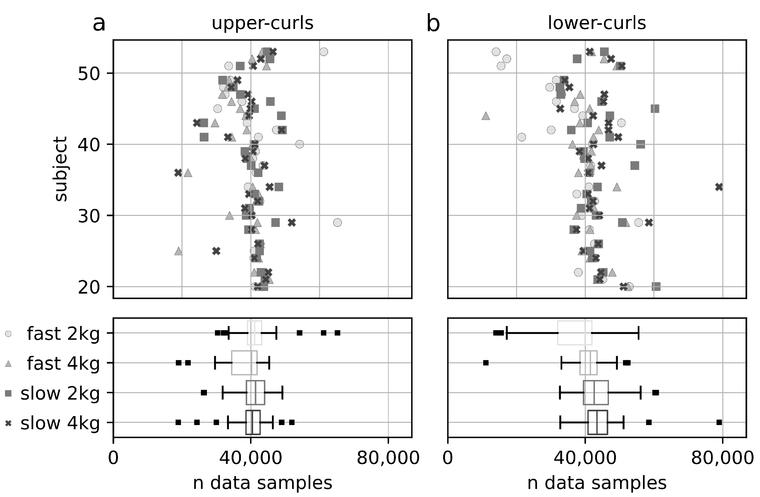
2.1.1. Subjects and Exercises

sEMG data and the corresponding elbow joint angle $\theta$ were acquired for $n=30$ subjects (24 male, 3 female and 3 in none of these categories; see Appendix A 

Table A1. Overview of all subjects. Ages are given in whole years. All information is based on the statements of the individual subject. Maxima are marked in bold and minima in bold and italic.

	Age	Sex	Height in m	Weight in kg
subject_20	23	female	1.64	68.00
subject_21	25	male	1.76	75.00
subject_22	25	male	1.90	85.00
subject_24	24	male	1.83	60.00
subject_25	25	-	1.93	85.00
subject_26	25	male	1.80	65.00
subject_28	22	male	1.83	73.00
subject_29	26	male	1.76	80.00
subject_30	25	male	1.90	130.00
subject_31	26	-	1.77	67.00
subject_32	29	male	1.78	110.00
subject_33	25	male	1.87	90.00
subject_34	23	male	1.75	63.00
subject_36	26	female	1.75	67.00
subject_37	29	male	1.84	70.00
subject_38	24	male	1.80	75.00
subject_39	24	male	1.86	82.00
subject_40	25	male	1.82	68.00
subject_41	23	male	1.67	69.00
subject_42	23	male	1.87	81.00
subject_43	22	male	1.76	58.00
subject_44	25	male	1.86	85.00
subject_45	34	male	1.90	90.00
subject_46	27	-	1.96	105.00
subject_47	24	male	1.91	86.00
subject_48	28	male	1.86	98.00
subject_49	22	male	1.89	85.00
subject_51	24	male	1.94	79.00
subject_52	32	male	1.90	74.00
subject_53	23	female	1.60	47.00
mean	25.27	-	1.82	79.00
standard deviation	2.76	-	0.09	16.46

), while the subjects were performing different elbow-movement sequences with their dominant hand (28 right-handed and 2 left-handed). All subjects were healthy and did not have any prior neuronal diseases when the experiments were performed. The movement sequences consisted of two different arm exercises with each at two different loads and at two different speeds, resulting in a total of eight experimental conditions (see Appendix A 

Table A2. Listing of all experimental conditions per subject.

$\mathit{posture}$		$\mathit{speed}$		$\mathit{load}$
$\mathit{upper}\mathit{curls}$	$\mathit{lower}\mathit{curls}$	$\mathit{fast}$	$\mathit{slow}$	2 kg	4 kg
x	-	x	-	x	-
x	-	x	-	-	x
x	-	-	x	x	-
x	-	-	x	-	x
-	x	x	-	x	-
-	x	x	-	-	x
-	x	-	x	x	-
-	x	-	x	-	x

). The two different upper arm exercises performed were upper curls and lower curls and are referred to as postures in the following. Subjects were asked to perform each exercise by cyclically moving the lower arm in a sinusoidal manner using a metronome as a visual and auditory reference. Each exercise was repeated at two different frequencies, referred to as slow (0.25 Hz) and fast (0.5 Hz) speeds. Again, each posture/speed combination was performed with different additional loads, namely 2 and 4 kg. Exercise lengths varied due to muscle fatigue of the individual subjects. Due to this circumstance, the recorded data used varied in length per experimental condition and subject (Figure 2).

2.1.2. Recording of sEMG Data

Wireless EMG sensors (Delsys Trigno, Delsys, Inc., Boston, MA, USA) were used to record the muscle activity of each of the two heads of the biceps brachii (bic) and triceps brachii (tric), both involved in the actuation of the lower arm, with a sample rate of 1111 Hz while subjects were performing exercise repetitions. Before the placement of the sensors, the skin was cleaned using isopropyl alcohol and the innervation zones of the respective muscles were marked via pen and tape roller according to [23] in order to determine the adequate positioning of the sensors. After the preparation of the skin and the determination of the positional placement, the sEMG sensors were fixed with double-sided adhesive tape on the skin of the subjects. The interface between skin and electrodes was evaluated via instructing the subjects to separately contract the flexors and extensors of the upper arm and subsequent visual inspection of the signal quality. The sEMG signals were filtered using a Butterworth bandpass filter with cutoff frequencies of 4 and 400 Hz according to [24].

2.1.3. Measurement of the Elbow-Joint Angle

A passive measurement orthosis was used to record the elbow-joint angle $\theta$ while the subjects were performing the different motion sequences. The measurement orthosis was custom designed and 3D-printed in house from polylactic acid (PLA) plastic. The mounting points and the overall length of the orthosis were customizable to allow fitting to different arm geometries. The elbow-joint angle was determined using a 10 bit magnetic rotary position encoder (AS5043, ams AG, Premstaetten, Austria), which was aligned to the rotary axis of the elbow joint of the subject. The analog output of the rotary encoder was fed into a Trigno Analog Adapter (Delsys, Inc., Boston, MA, USA) to allow for synchronous recording of the elbow joint angle $\theta$ and the sEMG data with a sample rate of 1111 Hz.

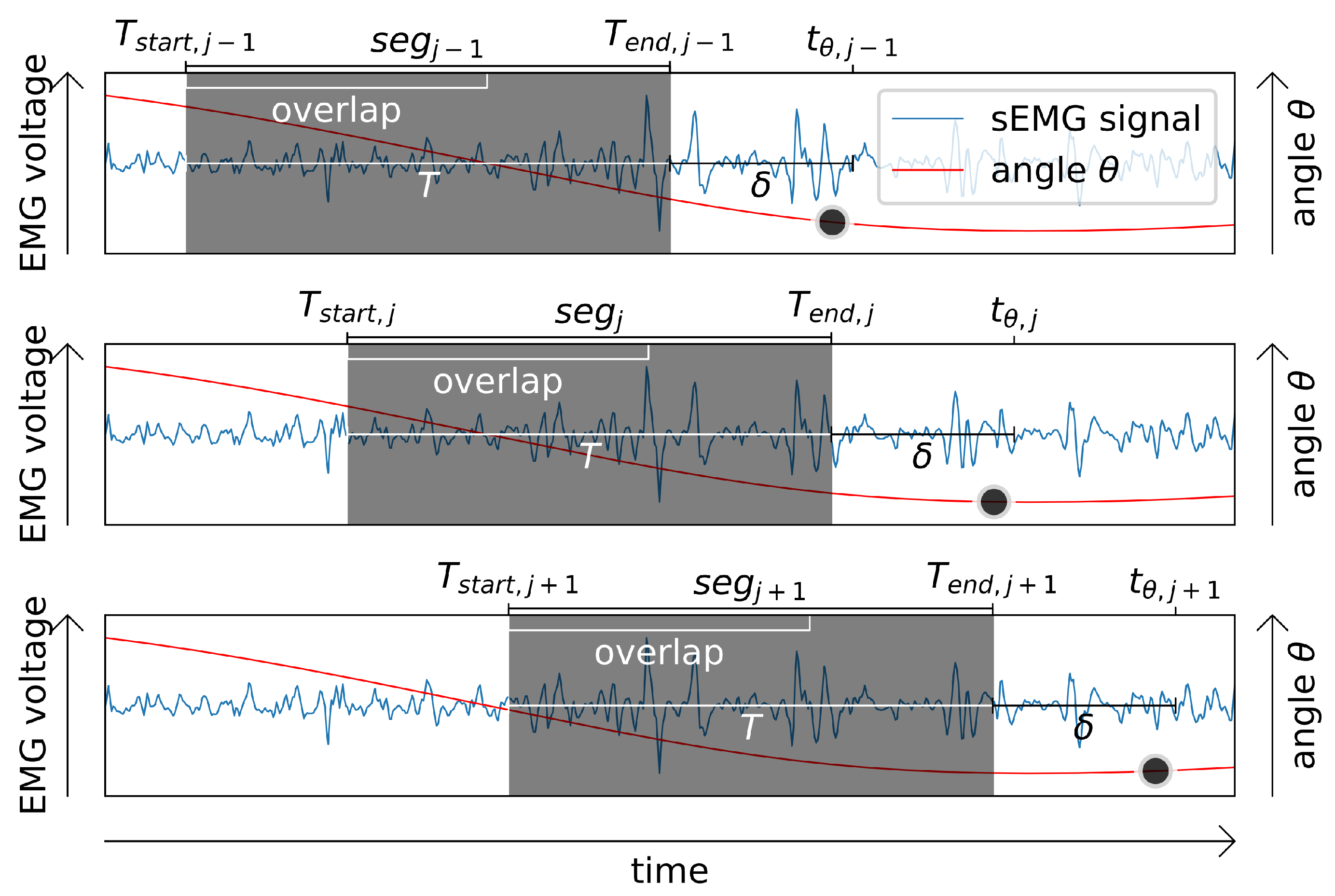
2.2. Segmentation of sEMG Data in the Time Domain

Muscle contraction is triggered via neural innervation of motor units, resulting in a release of acetylcholine (ACh) in the neuromuscular junction. It is followed by a biochemical cascade, leading to the formation of cross bridges, which extend from the myosin filaments and cyclically interact with actin filaments while adenosine triphosphate (ATP) is hydrolyzed [25,26,27]. Hence, a sEMG signal that activates the muscles involved in the actuation of the lower arm precedes the resulting movement of the elbow joint by approximately 50 to 100 ms due to the biochemical time constants [28,29]. As a result, the exact sEMG trigger signal corresponding to a predicted elbow-joint angle $\widehat{\theta }$ can only be approximated. Here, this approximation was achieved by choosing a time frame enclosing the corresponding sEMG trigger signal (Figure 3). This time frame will be referred to as segment, the number of data points contained within the segment as N, and the corresponding time span as segment length T in the following. By extracting single- or multiple features based on individual sEMG data segments, the increase in dimensionality of the input signal with respect to the input layer of the FFNN was compensated. To further account for the temporal latency between the sEMG trigger signal and the predicted elbow-joint angle $\widehat{\theta }$ due to biochemical and mechanical time constants as described above, a temporal offset $\delta$ was introduced according to

$$\delta =t_{\widehat{\theta }}-T_{end},$$

(1)

where $t_{\widehat{\theta }}$ is the point in time corresponding to the predicted elbow-joint angle $\widehat{\theta }$ and $T_{end}$ is the endpoint in time of the current segment (Figure 3).

As an additional segmentation parameter, the temporal overlap of segments in successive time steps (Figure 3) was considered. The maximal possible overlap depends on the overall sample frequency and is defined as being one data point less than the number of data points N in a segment of length T. Therefore, the overlap can be viewed as a hyperparameter controlling the frequency of feature signals. In all cases, the overlap was chosen such that features were sampled with a frequency of 100 Hz.

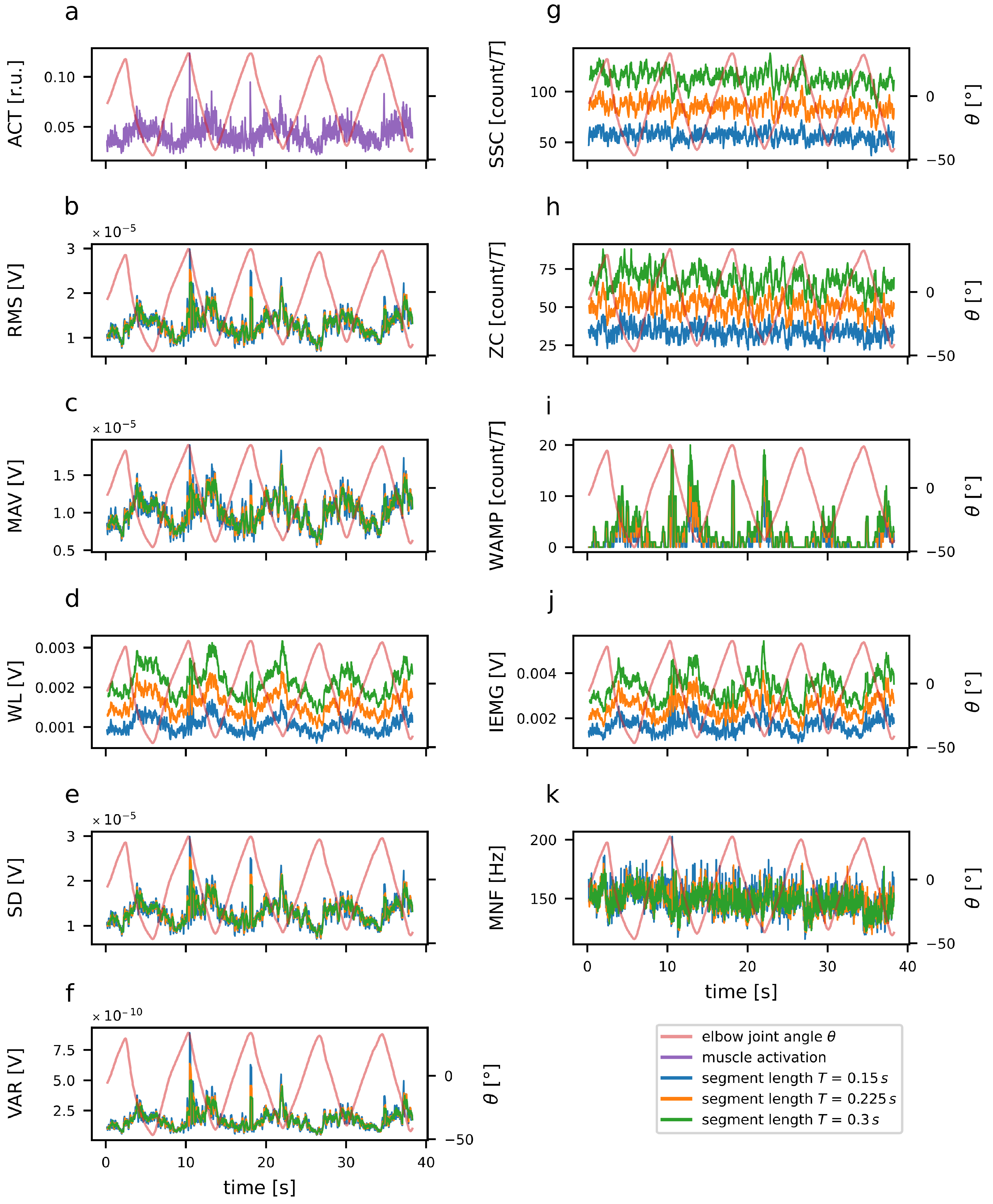
2.3. Signal Features for EMG-Based Movement Prediction

Different features were recently proposed for sEMG signal classification [19,21,22] and limb movement prediction [30]. The features were categorized as either time-domain (TD) or frequency-domain (FD) features and were used as single features or as feature sets composed of multiple features, so-called multi-feature sets. In this work, features within the three categories, time domain, frequency domain, and domain knowledge, were divided into subcategories based on their similarity to each other. All features, except the ACT feature (Section 2.3.1), were extracted after segmentation (Section 2.2) of the underlying sEMG signals.

2.3.1. Muscle Activation Dynamics

The muscle-activation (ACT) feature is a domain-knowledge-based feature, as it represents the biochemical cascade that relates the rate of change of muscle activation (i.e., calcium ion concentration in muscle) to the muscle excitation (i.e., firing of motor units), according to

$$\frac{du\left(t\right)}{dt}+\left[\frac{1}{{\tau }_{act}}·(\beta +[1-\beta ]e\left(t\right))\right]·u\left(t\right)=\left(\frac{1}{{\tau }_{act}}\right)·e\left(t\right),\mathrm{with}0<\beta <1,$$

(2)

where ${\tau }_{act}$ is the activation time constant and $\beta =\frac{\tau }{{\tau }_{deact}}$ is the ratio of activation to deactivation time constants, resulting in an asymmetric first-order low-pass filter [13,14]. ${\tau }_{act}$ and $\beta$ were set such that the step response matched the step response from the muscle-activation dynamics as described in [31] (${\tau }_{act}=17.3$ ms and $\beta =0.35$). The resulting muscle activity u is dimensionless and scaled between 0 ($u_{min}$) and 1 ($u_{max}$), corresponding to zero and maximal activation, respectively. The ACT feature was computed without prior segmentation of the sEMG signals, unlike the other EMG features (Figure 4a), but was downsampled to a frequency of 100 Hz in order to match the feature signal frequency due to the segment overlap parameter described in Section 2.2.

2.3.2. Features with Low-Pass Filter Character

Features characterized by low-pass filter-like behavior of the underlying functions were placed in a separate category: mean absolute value (MAV), root mean square (RMS), standard deviation (SD), variance (VAR), and waveform length (WL). All features of this category show similar temporal characteristics and differ mostly in magnitude.

Computing the root mean square from EMG signals is a standard procedure for extracting key information in diagnostics based on electromyography [32]. The RMS feature (Figure 4b) has also been used both as a single feature [16,17,33] and as a feature in a multi-feature set [19,22,30,34,35,36,37,38] for the myoelectric control of orthotic and prosthetic devices according to

$$RMS=\sqrt{{\displaystyle \frac{1}{N}\sum _{i=1}^N{x}_i^2}},$$

(3)

where N is the number of data pointsi within the segment under consideration, and x is the input data. The RMS feature is closely related to the MAV feature, which is part of the commonly used time domain (TD) feature set [19,30,34,35,36,37] and is computed from sEMG data segments (Figure 4c) according to

$${\displaystyle MAV=\frac{1}{N}\sum _{i=1}^N\left|x_i\right|.}$$

(4)

As another feature from the TD feature set, the waveform length WL was computed from sEMG data (Figure 4d), which is the cumulative length of the waveform over the time segment according to

$${\displaystyle WL=\sum _{i=1}^{N-1}\left|x_{i+1}-x_i\right|.}$$

(5)

WL is related to the waveform amplitude, frequency and time, and has been used in multi-feature sets [19,20,30,35,36,37,38].

The SD feature (i.e., the standard deviation of an input signal; Figure 4e),

$$SD=\sqrt{\frac{{\displaystyle \sum _{i=1}^N{\left|x_i-\overline{x}\right|}^2}}{N}},$$

(6)

which is defined as the square root of the variance of an input signal (i.e., VAR feature: Figure 4f)

$${\displaystyle VAR=\frac{1}{N}\sum _{i=1}^N{\left(x_i-\overline{x}\right)}^2,}$$

(7)

is considered as an alternative feature rather used in multi-feature sets [21,22,38,39].

2.3.3. Event-Based Features

Functions used for feature extraction in this subcategory depend on the occurrence of certain signal characteristics in a given segment of length T. Such event-based features used were signal slope changes SSC and zero crossings ZC, which both are members of the TD feature set [19,30,34,35,36,37] and are named based on the signal characteristic they represent, as well as the Willison amplitude (WAMP) [19,40].

The SSC feature (Figure 4g) depends on the number of occurrences of signal changes from a rising to falling slope and vice versa in the given data segment of length T according to

$$\begin{array}{c}{\displaystyle SSC=\sum _{i=2}^{N-1}{f}_{SSC}\left(x_i\right),}\end{array}$$

(8)

$$\begin{array}{c}{f}_{SSC}\left(x_i\right)=\left\{\begin{array}{cc}1\hfill & \mathrm{if}(x_i-x_{i-1})(x_i-x_{i+1})>0\hfill \\ 0\hfill & \mathrm{otherwise}\hfill \end{array}\right..\end{array}$$

(9)

The ZC feature (Figure 4h) depends on the number of occurrences of sign changes between data points according to

$$\begin{array}{c}{\displaystyle ZC=\sum _{i=1}^{N-1}{f}_{ZC}\left(x_i\right),}\end{array}$$

(10)

$$\begin{array}{c}{f}_{ZC}\left(x_i\right)=\left\{\begin{array}{cc}1\hfill & \mathrm{if}{x}_i{x}_{i+1}<0\hfill \\ 0\hfill & \mathrm{otherwise}\hfill \end{array}\right..\end{array}$$

(11)

The WAMP feature (Figure 4i) depends on the number of occurrences of how often a predefined threshold $\sigma$ ($=\pm 50\mathsf{\mu }$V; [40]) exceeds the difference among two successive amplitudes and, therefore, marks areas with wide amplitude ranges:

$$\begin{array}{c}{\displaystyle WAMP=\sum _{i=1}^{N-1}{f}_{WAMP}\left(x_j\right),}\end{array}$$

(12)

$$\begin{array}{c}{f}_{WAMP}\left(x_i\right)=\left\{\begin{array}{cc}1\hfill & \mathrm{if}\left|x_{i+1}-x_i\right|>\sigma \hfill \\ 0\hfill & \mathrm{otherwise}\hfill \end{array}\right..\end{array}$$

(13)

2.3.4. Integral-Based Features

The integral-based feature category consists of the integrated EMG (IEMG) feature (Figure 4j), which is defined as the absolute integral of the signal according to

$${\displaystyle IEMG=\sum _{i=1}^N\left|x_i\right|.}$$

(14)

In general, the IEMG is used as an index for the onset of muscle activity and is associated with the firing timing of the sEMG signal sequence [40].

2.3.5. Frequency Domain Features

The last subcategory is defined by features which are based on the distribution of power of the signal frequency components. The mean of signal frequencies MNF (Figure 4k) was proposed to be used as a single feature in classification by [19] and is computed according to

$$MNF=\frac{{\displaystyle \sum _{i=0}^n{I}_i·f_i}}{{\displaystyle \sum _{i=0}^n{I}_i}},$$

(15)

where n is the number of frequency bins in the spectrum of an applied fast Fast Fourier transform (FFT) to a segment of the number of data points N in a segment of length T. In this case, i is the index of the frequency bin instead of a step in time. I is the intensity of the spectrum at a given bin and f is the frequency at a given bin.

Though the MNF feature yielded rather inferior results compared to other features in recent classification tasks [19], it was not discarded in this paper, as frequency domain features potentially yield relevant information for movement prediction and might supplement time domain features in multi-feature sets.

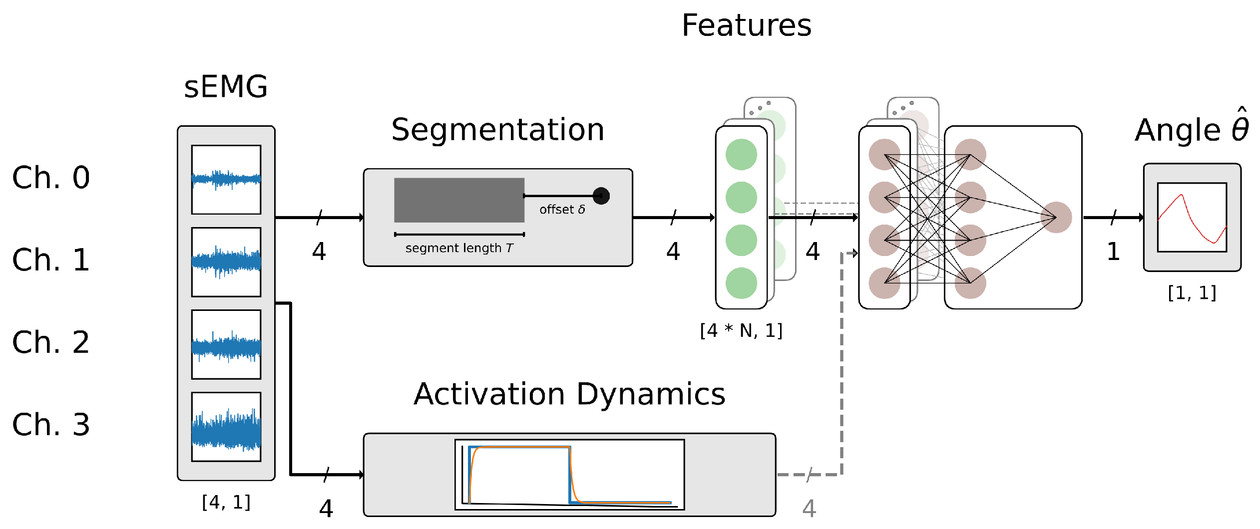
2.4. Feedforward Neural Network

In order to compare the influence of different sEMG signal features and segmentation parameters for the prediction of elbow-joint movement, a simple feedforward neural network (FFNN) was used. The network was implemented using the data stream oriented machine learning library TensorFlow (version 2.5.0; [41]) in Python (version 3.9.5; [42]). To ensure the comparability of models with different numbers of feature inputs, the structure of the FFNN was fixed depending on the number of features used (Figure 1). Each model consisted of two hidden layers. The number of neurons N of the input layer $N_{input}$ was defined as the product of the number of input channels $N_{channels}$, corresponding to the number of muscle heads recorded (Section 2.1.2) and the number of features $N_{features}$ used depending on whether single- or multi-feature sets were used for the performance evaluation according to

$$N_{input}=N_{channels}·N_{features}.$$

(16)

The hidden layer consisted of a fixed number of neurons $N_{hidden}$ equal to the number of input channels $N_{channels}$:

$$N_{\mathit{hidden}}=N_{\mathit{channels}}.$$

(17)

The number of output layer neurons was determined by the dimensionality of the predicted elbow joint angle $\widehat{\theta }$ and consequently was set to $N_{output}=1$. Within the hidden layer, all neurons used a hyperbolic tangent function (tanh) as the activation function; hence, the input signals were normalized to a range of $-1$ to 1. During training, the mean square error (MSE) was used as a loss function to determine whether a model was over- or underfit. As a model optimizer, the RMSprop algorithm from the Tensorflow toolkit [41] was chosen with a learning rate of $0.001$. Each model was initialized with random weights and biases and then trained for 1000 epochs. Learning terminated early if no improvement occurred for 20 epochs. Three models per experimental condition and subject combination were trained with 70% of the entire data set and tested with the remaining 30%. In total, 10% of the training set was used as a validation set during training. The data was not shuffled during the training test split to ensure that the model did not see at least one period of arm motion during training. The feedforward model architecture used was limited in the number of hidden layers and neurons per hidden layer to allow for the execution of a variety of different model evaluations and the time required to train one model per evaluation. Further, more complex models might have run the risk of overfitting due to a larger number of trainable hyperparameters [43].

2.5. Comparative Rating Metric

A normalized version of the mean absolute error (MAE), namely $nMAE$ (Equation (19)), was used to compare the prediction accuracy of the models trained with different sEMG signal features and segmentation parameters. The $MAE$ on which the $nMAE$ is based is defined as

$$MAE=\frac{{\sum }_{i=1}^N|\widehat{\theta }-\theta |}{N},$$

(18)

where $\widehat{\theta }$ is the predicted elbow-joint angle and $\theta$ is the corresponding experimentally recorded elbow-joint angle. In this case, N is the total number of evaluated predicted angles.

The normalization in $nMAE$ was achieved by

$$nMAE=\frac{MAE}{max\left(\theta \right)-min\left(\theta \right)}.$$

(19)

The nMAE was calculated for model predictions using the test data set ($nMAE$) as well as the train data set ($nMA{E}_{train}$). The prediction error $nMAE$ was used in the evaluation of all feature configurations and segmentation tests described in Section 3.1, Section 3.2 and Section 3.3 and was compared with the $nMA{E}_{train}$ to evaluate the model fitting. To evaluate the model performance for different feature configurations (single and multi-features) and segmentations, the mean $nMAE$ of all models that differ in terms of experimental conditions or subjects was used.

3. Results

The performance of the elbow-joint movement prediction using the FFNN architecture described in Section 2.4 was determined via a comparative rating metric (Section 2.5). The accuracy of the FFNN models with respect to single features was evaluated (Section 3.1) by comparing their predictive performance based on feature subcategories described in Section 2.3. Subsequently, single features that resulted in the highest predictive accuracy were used to determine the influence of different segmentation parameters (Section 3.2) on model performance. Finally, the predictive power of different multi-feature sets was compared based on a forward selection (Section 3.3). In all evaluations, a single model per experimental condition and subject combination was trained and evaluated.

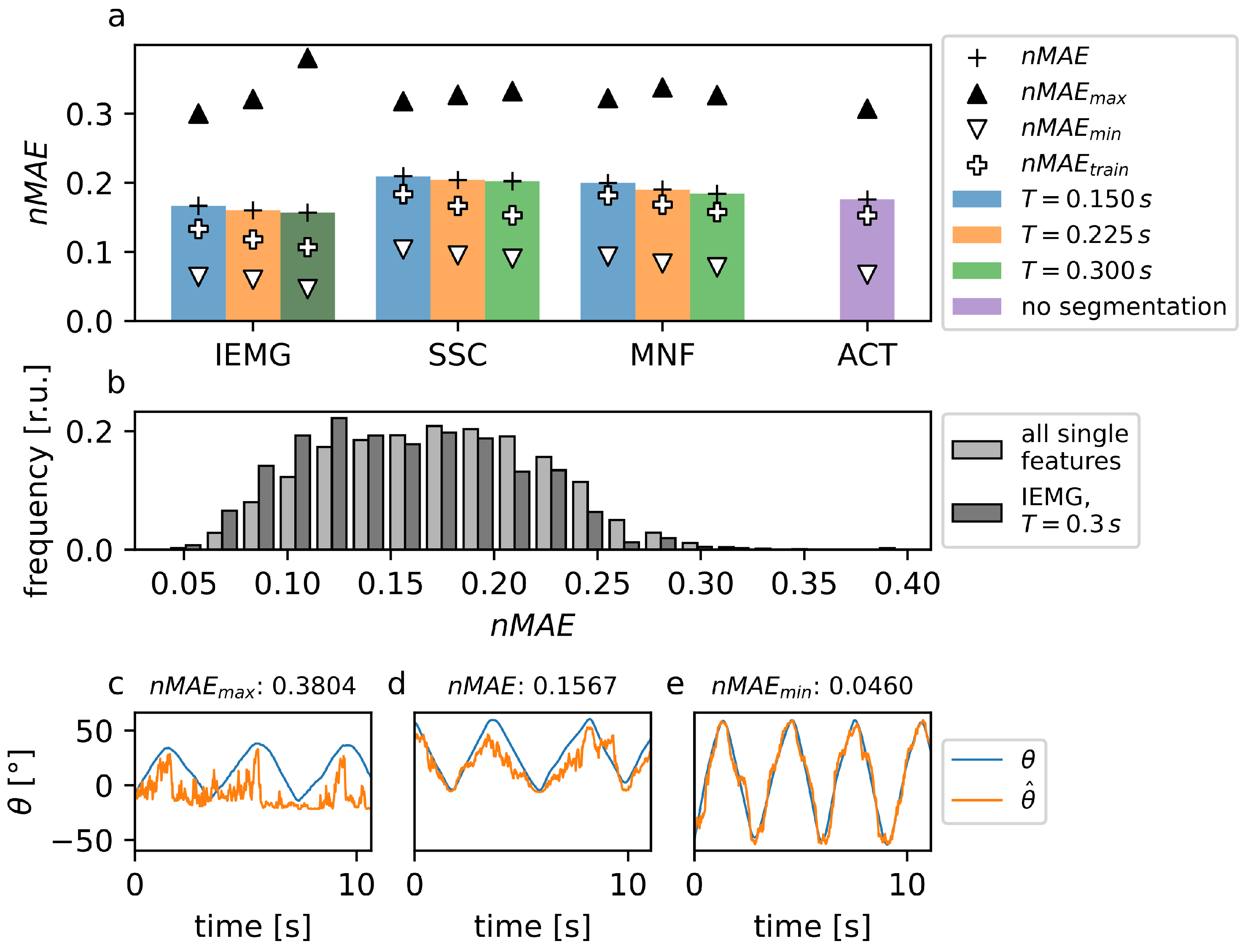
3.1. Single Features

The performance of models trained with individual single feature sets was compared to determine the features that yielded the best prediction accuracy, thereby presumably providing the most relevant information for motion prediction using the FFNN architecture described in Section 2.4. One feature out of each feature category (Section 2.3) was selected initially. It should be noted that although the IEMG feature (Equation (14)) was placed in a separate feature category (integral-based features; Section 2.3.4) due to its offset characteristics, it effectively equals the MAV feature (Equation (4)) due to the normalization inherent to the model architecture of the FFNN (Section 2.4). Hence, the IEMG feature was selected representatively for both groups (features with low-pass filter character and integral-based features), as it lacks one scaling operation, compared to the MAV feature and, therefore, is less prone to rounding errors. Out of the group categorizing event-based features, the SSC feature was chosen because it is less prone to drifts of the DC portion of the sEMG signal than the ZC feature, and the WAMP feature with its threshold $\sigma$ (Equation (12)) has an additional hyperparameter which increases the complexity. From the remaining subcategories, the MNF and ACT features were selected. Single features were compared using three distinct segment lengths T = [0.15 s, 0.225 s, 0.3 s]. This range of segment lengths was chosen based on previous findings, which used a mean segment length of (T=) $0.2265$ s [17,18,19,20,21,35,37,40].

In general, models trained with the widest segment length ($T=0.3$ s) yielded the lowest prediction error ($nMAE$) for all features when predicting elbow-joint movements as compared to shorter segment lengths (Figure 5). As the ACT feature does not depend on the segment length (Section 2.3.1), only a single prediction error could be computed. When trained with the IEMG feature, the prediction accuracy of the FFNN model yielded the lowest prediction error ($nMAE$) across all experimental conditions for all segment lengths and, hence, the highest accuracy in predicting the elbow-joint angle $\widehat{\theta }$. The lowest prediction error of ($nMAE=$) $0.1567$, and thus the highest prediction accuracy, was achieved when using the IEMG feature and a segment length of $(T=)$ 0.3 s. The ACT feature provided the second-best prediction accuracy with a prediction error of ($nMAE=$) $0.1757$. The SSC feature yielded the lowest prediction accuracy with a prediction error of ($nMAE=$) $0.2093$ using the shortest tested segment length of $(T=)$$0.15$ s. A comparison of the mean of prediction errors for the training ($\overline{nMA{E}_{train}}$) and test data sets ($\overline{nMAE}$) shows that models generally fitted well. Neither significant under- nor over-fitting occurred, as the prediction of previous unseen data resulted in a similar mean of prediction error ($\overline{nMAE}=0.1848$) values, compared to the seen data ($\overline{nMA{E}_{train}}=0.1521$). This implies that the chosen model structure is suitable for predicting elbow-joint movements based on the sEMG data as described above.

3.2. Segmentation

Based on the IEMG feature, which provided the best prediction accuracy in the evaluation of prediction performance based on single features, the influence of the segment length T and the offset $\delta$ on the prediction performance of the FFNN model was analyzed subsequently. Special consideration was given to the fact that the two different movement speeds at which the subjects performed the exercises resulted in different period lengths of the elbow-joint angle $\theta$ (fast: $2.5$ s, slow: 5 s; Section 2.1). The choice of segment lengths T in this context was therefore based on the assumption that for periodic movements with a fixed frequency, segment lengths with up to half a period in length result in a higher prediction accuracy since they have the greatest information content retrospectively to make a prediction about the future course of the signal. To test this assumption, segments with a zero offset ($\delta =0$), based on half a period (2.5 s) of a slow movement condition, were systematically varied in the length of segment T and evaluated with regard to their predictive accuracy. Subsequently, the boundary $T_{end}$ (see Figure 3) of segments with the segment length that gave the highest prediction accuracy was systematically shifted, leading simultaneously to (a) an offset $\delta$ of the segment as well as (b) to a further decrease in segment lengthT corresponding to the step size of the shift of the boundary value ($T-\delta$). The predictive accuracy of the model was then re-evaluated with respect to the shift of the segment boundary $T_{end}$.

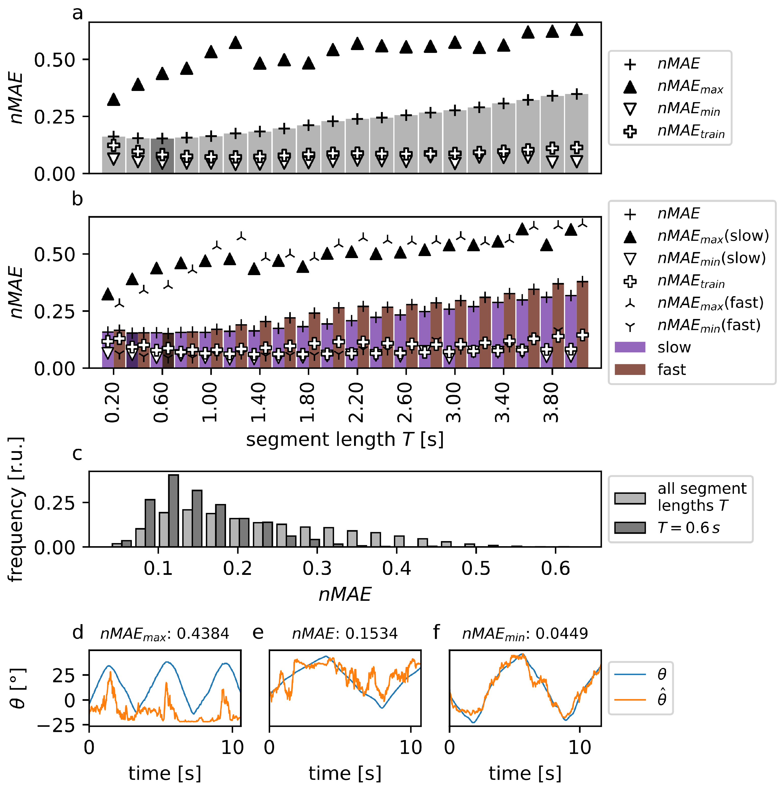
3.2.1. Evaluation of Segment Length

As a first step in the evaluation of segmentation parameters, the length of sEMG data segments with no offset ($\delta =0$) was varied between T = [0.2 s…4.0 s] with a step width of 0.2 s. With a segment length of ($T=$) 0.6 s the lowest prediction error ($nMAE=0.1532$) and thus the best prediction accuracy was achieved after training the FFNN (Figure 6). Starting from this segment length, both increments and decrements of the segment length T led to a deterioration of the prediction accuracy, corresponding to a prediction error of ($nMAE=$) $0.1619$ for the shortest segment length ($T=0.2$ s) and a prediction error of ($nMAE=$) $0.3481$ for the widest segment length ($T=4.0$ s) tested. This observation persisted, even if the prediction accuracy was plotted separately based on the movement speed by which exercises were performed (see Figure 6b). Thus, a segment length of ($T=$) $0.4s$ resulted in the lowest prediction error ($nMAE=0.1535$) for the slow condition and a segment length of ($T=$) $0.6s$ resulted in the lowest prediction error ($nMAE=0.1513$) for the fast condition. However, it can be observed that the prediction accuracy as a function of motion speed deteriorated more strongly with a wider segment length when the exercises were performed with a fast movement speed as compared to when performed with a slow movement speed. This results in the highest prediction error, and thus the lowest prediction accuracy, for a segment length of ($T=$) 4.0 s, for both the slow ($nMAE=0.3174$) and fast ($nMAE=0.3787$) conditions.

Evaluation of the prediction errors for the training ($nMA{E}_{train}$) and test ($nMAE$) data sets as shown in Figure 6 makes clear that the chosen model structure tended to overfit at larger segment lengths and without offsets, as the difference between the prediction errors of the training $nMA{E}_{train}$ and test data sets $nMAE$ starts to increase with increasing segment length T. This effect can be attributed to the fact that with larger segment lengthsT, the number of total data samples per experiment decreased and the training data sets became too small for the model to generalize.

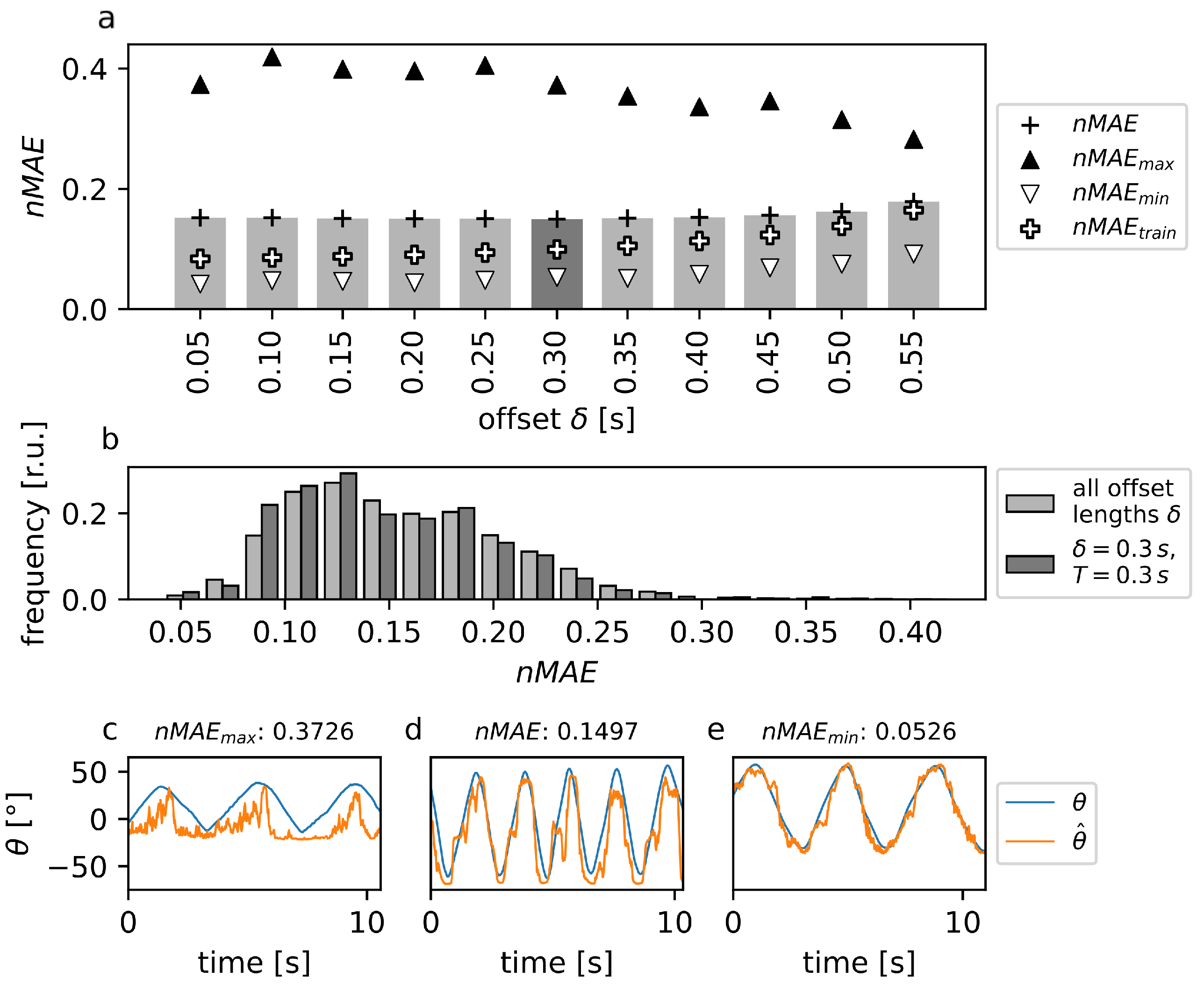
3.2.2. Evaluation of the Segment Boundary Offset

Following the evaluation of the segment length, the shift of the segment boundary $T_{end}$ was assessed with respect to the prediction accuracy of the FFNN. A segment length of ($T=$) 0.6 s was used as a basis, which in the previous performance evaluation provided the lowest prediction error ($nMAE$) under consideration of the IEMG feature. Based on this parameter combination, the segment length was successively decreased by shifting the segment boundary $T_{end}$, introducing an offset $\delta$ between the predicted elbow-joint angle $\widehat{\theta }$ and the segment boundary $T_{end}$, as well as a decrease in segment length ($T-\delta$).

In a parameter variation, the segment boundary was shifted with a step size of 0.05 s in the range of [0.05 s…0.55 s], and the prediction accuracy of the model after training with this feature combination was determined. The lowest prediction error ($nMAE=0.1496$) was achieved with a shift of the segment boundary (and thus an offset $\delta$) of 0.3 s and a resulting segment length of ($T=$) 0.3 s (Figure 7), which represents an improvement in the prediction accuracy compared to no shift of the segment boundary $T_{end}$ (Section 3.2.1). However, when comparing the prediction performance based on the shift of the segment boundary $T_{end}$ for the offsets $\delta$ and corresponding segment lengthT tested in Figure 7, there is little difference in terms of the prediction accuracy, as prediction errors show only a small variance ($\sigma =0.00825$). It should be noted that with a smaller segment length T (and, correspondingly, larger offset $\delta$) the prediction error increased, resulting in a maximum prediction error of ($nMAE=$) $0.1789$ with an offset of ($\delta =$) 0.55 s and a corresponding segment length of ($T=$) 0.05 s. Examining the prediction accuracy with respect to the training and test data sets shows that the difference between the prediction errors $nMAE$ and $nMA{E}_{train}$ is larger if smaller offsets are used; hence, larger segment lengthsT led to a stronger tendency of the model to overfit.

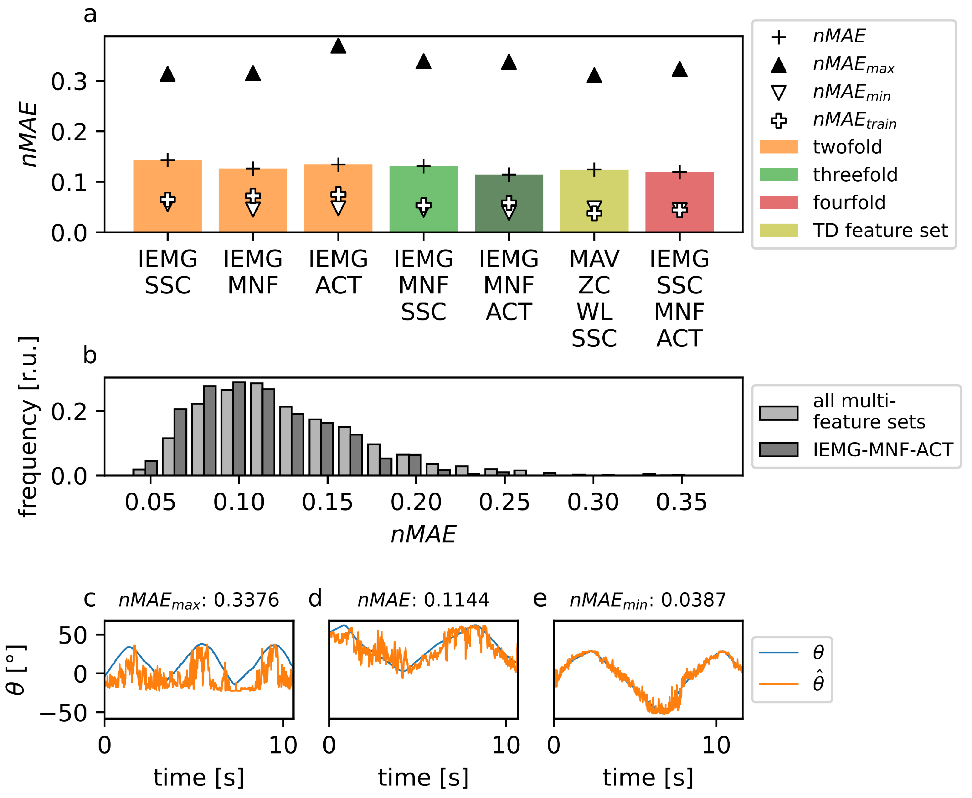
3.3. Multi-Feature Sets

Based on the determination of single features and segmentation parameters that led to the highest predictive performance of the model, a further step was taken to investigate whether combinations of single features, via so-called multi-feature sets, led to a further improvement in predictive performance. Hence, the IEMG feature that yielded the best predictive performance of the model as a single feature was systematically combined in a forward selection with the remaining features of the single-feature selection (see Section 3.1). In this process, the segmentation parameters were chosen to correspond to the parameters that provided the highest prediction accuracy in the segmentation parameter selection ($\delta =0.3$ s and $T=0.3$ s; see Section 3.2). Subsequently, based on the feature combination yielding the highest prediction accuracy in each forward selection step, the number of features was increased. This resulted in sets of twofold, threefold and fourfold multi-feature combinations, which were evaluated regarding the predictive performance of the model based on the mean absolute prediction error (Figure 8). Further, the TD feature set (including MAV, ZC, WL and SSC features; [19,30,34,35,36,37]) was also tested using the segmentation parameters, yielding the best predictive performance of the FFNN in Section 3.2 as a reference.

When comparing the predictive accuracy of the model for twofold multi-feature combinations (i.e., IEMG-SSC, IEMG-MNF and IEMG-ACT; Figure 8), the combination of an integral-based and a frequency-domain feature (IEMG-MNF) resulted in the lowest prediction error of the model ($nMAE=0.1262$). In contrast, the feature combination of the integral-based and event-based feature (IEMG-SSC) resulted in the highest prediction error of the model ($nMAE=0.1428$). It should be noted that the twofold multi-feature sets tested generally resulted in an improvement of the predictive performance of the model compared to the single IEMG feature with an offset of ($\delta =$) 0.3 s and a segment length of ($T=$) 0.3 s as described in the previous section (Section 3.2).

In the subsequent combinations of the IEMG-MNF feature to threefold feature sets during forward selection, it was found again that a combination with the event-based feature (IEMG-MNF-SSC) led to the lowest prediction performance ($nMAE=0.1310$). However, a combination with the domain knowledge-based feature (IEMG-MNF-ACT) led to a further improvement in the prediction performance ($nMAE=0.1143$, Figure 8) as compared to the prediction performance based on twofold feature sets as described above.

Perhaps unsurprisingly, the combination of the IEMG-MNF-ACT feature set with the event-based SSC feature, which already provided the worst prediction performance in the previous forward selection steps, did not result in any further improvement of the prediction error ($nMAE=0.1195$). However, the prediction accuracy for this fourfold multi-feature set (IEMG-SSC-MNF-ACT) still outperformed the accuracy of the FFNN model trained with the commonly used TD feature set ($nMAE=0.1243$, Figure 8) using the segmentation parameters, yielding the best prediction accuracy as described in Section 3.2.

4. Discussion

In this paper, various single features, combinations of single features and segmentation parameters of sEMG data were evaluated with respect to the accuracy of a simple FFNN model for the prediction of elbow-joint angles. It was shown that certain single features provide higher model performance in terms of prediction accuracy than others (Section 3.1). Thereby, the accuracy of the prediction also depends on the segment length T and the offset $\delta$ (with respect to the predicted elbow-joint angle $\widehat{\theta }$) of the segments from which features are extracted (Section 3.2). By combining individual features into multi-feature sets, the prediction accuracy can further be increased (Section 3.3). The sEMG features and segmentation parameters found using the method described above outperform the TD feature set commonly used in the literature in terms of predictive accuracy for the task at hand. Further, sEMG signal features, such as SSC, could be identified, which might not be suitable for the prediction of elbow-joint angles using FFNN, as they deteriorate predictive performance when used in multi-feature sets (Figure 8).

It should be noted, however, that within the procedure presented here, the selection of features and parameters that provided the highest prediction accuracy was always based on the previous selection step. For example, for the IEMG feature, which provided the highest prediction accuracy in the single feature selection (see Figure 5), the optimal segment length T (Figure 6), the segment offset $\delta$ (Figure 7), as well as the optimal additional features for combination (IEMG-MNF-ACT; Figure 8) could be determined, but the validity of those parameters for the other features considered here cannot be derived from this. Furthermore, a statement about the prediction accuracy can only be made in connection with the investigated experimental conditions and the architecture of the neural network used. Thus, it cannot be excluded and is also plausible that, for example, other segment lengths, for different features or motion speed paradigms than the ones used here might provide better results in terms of prediction accuracy since they control, for example, for low-pass-like features the smoothing of the signal as well as the frequency content of the individual segments.

Nevertheless, the present evaluation shows that a prior feature and parameter selection can provide better prediction accuracy with respect to limb movement prediction based on sEMG data than by using feature sets that are commonly used in the literature. Thus, when using the same segmentation parameters, the IEMG-MNF-ACT feature identified here provided a higher prediction accuracy than the TD feature set (see Figure 8), which was established for sEMG-based limb movement prediction in previous studies. Since this multi-feature set is a combination of individual features from the time-, frequency-, and domain-knowledge-based categories, it can be concluded that a selection of features representing different sEMG signal properties can be beneficial in terms of the predictive accuracy of a model. Still, the combination with features from other categories can also worsen the prediction performance. For example, a combination of the IEMG-MNF-ACT feature set with the SSC feature from the event-based category, which also had the lowest prediction accuracy in the single feature selection, resulted in a slight deterioration of the prediction performance of the model used here (see Figure 8). This is possibly due to the fact that the number of signal slope changes, as represented by the SSC feature in a segment, has little predictive power over the continuous waveform of a sEMG signal. Accordingly, when selecting features, care should be taken to determine whether they encode relevant signal properties.

Interestingly, with respect to the segmentation parameters yielding the highest predictive accuracy for the IEMG feature ($\delta$ = 0.3 s, T = 0.3 s), it was found that the offset of the segment and, thus, the time window for the prediction of the elbow-joint angle ($\widehat{\delta }$) from the sEMG data was outside the range of latency values of 50 to 100 ms reported in the literature [28,29]. This latency, however, is attributed to the time constant of the muscle activation dynamics and therefore covers the time span from EMG onset to the onset of muscle force and, consequently, to the onset of joint torque. However, besides the (biochemical) time constant of the muscle activation dynamics, the offset $\delta$ also has to cover additional time constants, for instance, of the biomechanical properties of the limb to generate movement from torque. Additionally, during the experimental acquisition of the sEMG data, additional time constants, such as those attributed to the slack of the retaining strap of the measurement orthosis, were introduced. Latency measurements performed in our laboratory with different measurement orthoses confirm this assumption (not published).

For the purposes of comparability of single features and multi-feature combinations as well as segmentation parameters, the neural network architecture was fixed with respect to the number of neurons involved. The predictive accuracy of different model architectures was explicitly not investigated in this work. Furthermore, one network was trained for each experimental condition and for each subject. For a further investigation of the predictive ability with respect to limb movement based on sEMG data, it would accordingly be interesting to investigate more complex model architectures and, based on larger data sets, to evaluate these models based on their ability to generalize with respect to different movement paradigms and/or multiple subjects. Furthermore, the features examined here represent only a small selection of possible features used in the literature. For a more thorough investigation, the feature selection method used here could be extended with other features, such as autoregressive coefficients, which potentially yield relevant information for the prediction of limb movement based on sEMG data.

References

1. Aida, T.; Nozaki, H.; Kobayashi, H. Development of muscle suit and application to factory laborers. In Proceedings of the 2009 International Conference on Mechatronics and Automation, Changchun, China, 9–12 August 2009; pp. 1027–1032. [Google Scholar] [CrossRef]
2. Kim, W.; Lee, H.; Lim, D.; Han, J.; Han, C. Development of a Lower Extremity Exoskeleton System for Walking Assistance While Load Carrying. In WORLD SCIENTIFIC Proceedings of the 16th International Conference on Climbing and Walking Robots and the Support Technologies for Mobile Machines-University of Technology Sydney, Australia, 14–17 July 2012; World Scientific: Singapore, 2013; pp. 35–42. [Google Scholar] [CrossRef]
3. Silveira, A.; Abreu de Souza, M.; Fernandes, B.; Nohama, P. From the past to the future of therapeutic orthoses for upper limbs rehabilitation. Res. Biomed. Eng. 2018, 34, 368–380. [Google Scholar] [CrossRef]
4. Pundik, S.; McCabe, J.; Kesner, S.; Skelly, M.; Fatone, S. Use of a myoelectric upper limb orthosis for rehabilitation of the upper limb in traumatic brain injury: A case report. J. Rehabil. Assist. Technol. Eng. 2020, 7, 2055668320921067. [Google Scholar] [CrossRef] [PubMed]
5. Wehner, M.; Rempel, D.; Kazerooni, H. Lower Extremity Exoskeleton Reduces Back Forces in Lifting. In WORLD SCIENTIFIC Proceedings of the 16th International Conference on Climbing and Walking Robots and the Support Technologies for Mobile Machines, University of Technology Sydney, Sydney, Australia, 14–17 July 2012; World Scientific: Singapore, 2013; pp. 49–56. [Google Scholar] [CrossRef]
6. Hasegawa, Y.; Muramatsu, M. Wearable lower-limb assistive device for physical load reduction of caregiver on transferring support. In Proceedings of the 2013 IEEE/ASME International Conference on Advanced Intelligent Mechatronics, Wollongong, NSW, Australia, 9–12 July 2013; pp. 1027–1032. [Google Scholar] [CrossRef]
7. Tsuzura, M.; Nakakuki, T.; Misaki, D. A mechanism design of waist power assist suit for a caregiver by using torsion springs. In Proceedings of the 2013 13th International Conference on Control, Automation and Systems (ICCAS 2013), Gwangju, Korea, 20–23 October 2013; pp. 866–868. [Google Scholar] [CrossRef]
8. Giovacchini, F.; Vannetti, F.; Fantozzi, M.; Cempini, M.; Cortese, M.; Parri, A.; Yan, T.; Lefeber, D.; Vitiello, N. A light-weight active orthosis for hip movement assistance. Robot. Auton. Syst. 2015, 73, 123–134. [Google Scholar] [CrossRef]
9. Boschmann, A.; Platzner, M. Towards robust HD EMG pattern recognition: Reducing electrode displacement effect using structural similarity. In Proceedings of the 2014 36th Annual International Conference of the IEEE Engineering in Medicine and Biology Society, Chicago, IL, USA, 26–30 August 2014; Volume 2014, pp. 4547–4550. [Google Scholar]
10. Kim, J.; Koo, B.; Nam, Y.; Kim, Y. sEMG-Based Hand Posture Recognition Considering Electrode Shift, Feature Vectors, and Posture Groups. Sensors 2021, 21, 7681. [Google Scholar] [CrossRef]
11. Li, Z.; Zhao, X.; Liu, G.; Zhang, B.; Zhang, D.; Han, J. Electrode Shifts Estimation and Adaptive Correction for Improving Robustness of sEMG-Based Recognition. IEEE J. Biomed. Health Inform. 2021, 25, 1101–1110. [Google Scholar] [CrossRef]
12. Hill, A.V. The effect of load on the heat of shortening of muscle. Proc. R. Soc. Lond. Ser. Biol. Sci. 1964, 159, 297–318. [Google Scholar]
13. Zajac, F.E. Muscle and tendon: Properties, models, scaling, and application to biomechanics and motor control. Crit. Rev. Biomed. Eng. 1989, 17, 359–411. [Google Scholar]
14. Buchanan, T.S.; Lloyd, D.G.; Manal, K.; Besier, T.F. Neuromusculoskeletal modeling: Estimation of muscle forces and joint moments and movements from measurements of neural command. J. Appl. Biomech. 2004, 20, 367–395. [Google Scholar] [CrossRef] [Green Version]
15. Côté-Allard, U.; Fall, C.L.; Drouin, A.; Campeau-Lecours, A.; Gosselin, C.; Glette, K.; Laviolette, F.; Gosselin, B. Deep Learning for Electromyographic Hand Gesture Signal Classification Using Transfer Learning. IEEE Trans. Neural Syst. Rehabil. Eng. 2019, 27, 760–771. [Google Scholar] [CrossRef] [Green Version]
16. Aung, Y.M.; Al-Jumaily, A. Estimation of Upper Limb Joint Angle Using Surface EMG Signal. Int. J. Adv. Robot. Syst. 2013, 10, 369. [Google Scholar] [CrossRef] [Green Version]
17. Kiguchi, K.; Hayashi, Y. An EMG-Based Control for an Upper-Limb Power-Assist Exoskeleton Robot. IEEE Trans. Syst. Man. Cybern. B Cybern. 2012, 42, 1064–1071. [Google Scholar] [CrossRef]
18. El-Khoury, S.; Batzianoulis, I.; Antuvan, C.W.; Contu, S.; Masia, L.; Micera, S.; Billard, A. EMG-based learning approach for estimating wrist motion. In Proceedings of the 2015 37th Annual International Conference of the IEEE Engineering in Medicine and Biology Society (EMBC), Milan, Italy, 25–29 August 2015; pp. 6732–6735. [Google Scholar] [CrossRef] [Green Version]
19. Oskoei, M.A.; Hu, H. Support Vector Machine-Based Classification Scheme for Myoelectric Control Applied to Upper Limb. IEEE Trans. Biomed. Eng. 2008, 55, 1956–1965. [Google Scholar] [CrossRef]
20. López-Delis, A.; Ruiz-Olaya, A.F.; Freire-Bastos, T.; Delisle-Rodríguez, D. A Comparison of Myoelectric Pattern Recognition Methods to Control an Upper Limb Active Exoskeleton. In Progress in Pattern Recognition, Image Analysis, Computer Vision, and Applications; Ruiz-Shulcloper, J., Sanniti di Baja, G., Eds.; Springer: Berlin/Heidelberg, Germany, 2013; pp. 100–107. [Google Scholar] [CrossRef]
21. David Orjuela-Cañón, A.; Ruíz-Olaya, A.F.; Forero, L. Deep neural network for EMG signal classification of wrist position: Preliminary results. In Proceedings of the 2017 IEEE Latin American Conference on Computational Intelligence (LA-CCI), Arequipa, Peru, 8–10 November 2017; pp. 1–5. [Google Scholar] [CrossRef]
22. Akhundov, R.; Saxby, D.J.; Edwards, S.; Snodgrass, S.; Clausen, P.; Diamond, L.E. Development of a deep neural network for automated electromyographic pattern classification. J. Exp. Biol. 2019, 222, jeb198101. [Google Scholar] [CrossRef] [Green Version]
23. Rainoldi, A.; Merletti, R.; Barbero, M. Atlas of Muscle Innervation Zones: Understanding Surface Electromyography and Its Applications; Springer: Milan, Italy, 2012. [Google Scholar]
24. Fuentes, S.; Wei, Y.; Olmeda, E.; Ren, L.; Wei, G.; Díaz, V. Validation of a Low-Cost Electromyography (EMG) System via a Commercial and Accurate EMG Device: Pilot Study. Sensors 2019, 19, 5214. [Google Scholar] [CrossRef] [Green Version]
25. Huxley, A.F.; Niedergerke, R. Structural changes in muscle during contraction: Interference microscopy of living muscle fibres. Nature 1954, 173, 971–973. [Google Scholar] [CrossRef]
26. Huxley, H.; Hanson, J. Changes in the cross-striations of muscle during contraction and stretch and their structural interpretation. Nature 1954, 173, 973–976. [Google Scholar] [CrossRef]
27. Lymn, R.; Taylor, E.W. Mechanism of adenosine triphosphate hydrolysis by actomyosin. Biochemistry 1971, 10, 4617–4624. [Google Scholar] [CrossRef]
28. Inman, V.T.; Ralston, H.J.; Saunders, J.B.; Feinstein, B.; Wright, E.W.J. Relation of human electromyogram to muscular tension. Electroencephalogr. Clin. Neurophysiol. 1952, 4, 187–194. [Google Scholar] [CrossRef]
29. Howatson, G. The impact of damaging exercise on electromechanical delay in biceps brachii. J. Electromyogr. Kinesiol. 2010, 20, 477–481. [Google Scholar] [CrossRef]
30. Pulliam, C.L.; Lambrecht, J.M.; Kirsch, R.F. Electromyogram-based neural network control of transhumeral prostheses. J. Rehabil. Res. Dev. 2011, 48, 739–754. [Google Scholar] [CrossRef]
31. Winters, J.M. An improved muscle-reflex actuator for use in large-scale neuro-musculoskeletal models. Ann. Biomed. Eng. 1995, 23, 359–374. [Google Scholar] [CrossRef] [PubMed]
32. Luca, C.J.D. The Use of Surface Electromyography in Biomechanics. J. Appl. Biomech. 1997, 13, 135–163. [Google Scholar] [CrossRef] [Green Version]
33. Gupta, S.D. Estimation of Arm Joint Angles from Surface Electromyography signals using Artificial Neural Networks. IOSR J. Comput. Eng. 2013, 15, 38–44. [Google Scholar] [CrossRef]
34. Hudgins, B.; Parker, P.; Scott, R.N. A new strategy for multifunction myoelectric control. IEEE Trans. Biomed. Eng. 1993, 40, 82–94. [Google Scholar] [CrossRef]
35. Englehart, K.; Hudgins, B. A robust, real-time control scheme for multifunction myoelectric control. IEEE Trans. Biomed. Eng. 2003, 50, 848–854. [Google Scholar] [CrossRef]
36. Mattioli, F.E.R.; Lamounier, E.A.J.; Cardoso, A.; Soares, A.B.; Andrade, A.O. Classification of EMG signals using artificial neural networks for virtual hand prosthesis control. In Proceedings of the 2011 Annual International Conference of the IEEE Engineering in Medicine and Biology Society, Boston, MA, USA, 30 August–3 September 2011; Volume 2011, pp. 7254–7257. [Google Scholar]
37. Akhtar, A.; Hargrove, L.; Bretl, T. Prediction of distal arm joint angles from EMG and shoulder orientation for prosthesis control. In Proceedings of the 2012 Annual International Conference of the IEEE Engineering in Medicine and Biology Society, San Diego, CA, USA, 28 August–1 September 2012; Volume 2012, pp. 4160–4163. [Google Scholar] [CrossRef]
38. Ahsan, M.R.; Ibrahimy, M.; Khalifa, O. The Use of Artificial Neural Network in the Classification of EMG Signals. In Proceedings of the 2012 Third FTRA International Conference on Mobile, Ubiquitous, and Intelligent Computing, Vancouver, BC, Canada, 26–28 June 2012; pp. 225–229. [Google Scholar] [CrossRef]
39. Jahan, M.; Manas, M.; Sharma, B.B.; Gogoi, B.B. Feature extraction and pattern recognition of EMG-based signal for hand movements. In Proceedings of the 2015 International Symposium on Advanced Computing and Communication (ISACC), Silchar, India, 14–15 September 2015; pp. 49–52. [Google Scholar] [CrossRef]
40. Noble, J.; Retheep, R.; Adithya, P.K.; Sivanadan, K.S. Classification of forearm movements from sEMG time domain features using machine learning algorithms. In Proceedings of the TENCON 2017-2017 IEEE Region 10 Conference, Penang, Malaysia, 5–8 November 2017; pp. 1624–1628. [Google Scholar] [CrossRef]
41. Abadi, M.; Agarwal, A.; Barham, P.; Brevdo, E.; Chen, Z.; Citro, C.; Corrado, G.S.; Davis, A.; Dean, J.; Devin, M.; et al. TensorFlow: Large-Scale Machine Learning on Heterogeneous Systems. 2015. Available online: tensorflow.org (accessed on 5 February 2022).
42. Van Rossum, G.; Drake, F.L., Jr. Python Reference Manual; Centrum voor Wiskunde en Informatica: Amsterdam, The Netherlands, 1995. [Google Scholar]
43. Bejani, M.M.; Ghatee, M. A systematic review on overfitting control in shallow and deep neural networks. Artif. Intell. Rev. 2021, 54, 6391–6438. [Google Scholar] [CrossRef]
Figure 1. Schematic illustration of the procedure for evaluating different features and feature combinations, as well as segmentation parameters for predicting elbow-joint movement by an FFNN based on sEMG data. Depending on which features were evaluated, the sEMG data were either segmented, or directly processed by a muscle activation dynamics model. All features served either as single features, or in various multi-feature combinations as input signals to an FFNN that was trained to predict the corresponding angle of an elbow joint θ ^ . Note that the input layer of the FFNN scaled with the number of features used ( N i n p u t = N c h a n n e l s · N f e a t u r e s ).
Mathematics 10 00932 g001
Figure 2. Distribution of the number (n) of recorded sEMG data samples (sampling rate of 1111 Hz) for each subject separated by posture: (a) upper curls and (b) lower curls. The plots in the top row depict the data samples per individual subject. The boxplots in the lower row summarize the distribution of data samples based on experimental conditions (speed and load) for all subjects. Whiskers are plotted within the 1.5 interquartile range (IQR), and black dots represent outliers.
Mathematics 10 00932 g002
Figure 3. Exemplary representation of segment length T, offset  δ and overlap for three successive segmentation time steps j. Each of the three subplots represent the same sEMG signal (blue) and corresponding elbow-joint angle θ (red) in each row. The gray boxes symbolically represent a segment of the sEMG signal from which features were extracted in each segmentation time step j. Depending on the feature extracted, segments of length T were reduced in dimensionality and mapped to a corresponding predicted angle θ ^ (black dot) via the offset  δ . The overlap of segments between successive segmentation time steps j and j + 1 determines the frequency by which features were sampled.
Mathematics 10 00932 g003
Figure 4. Exemplary representation of features extracted from an sEMG data signal segmented based on three different segment lengths (blue: T = 0.15 s , orange: T = 0.225 s and green: T = 0.3 s ; purple: no segmentation), as well as the corresponding elbow-joint angle θ (red), recorded experimentally. The features depicted were extracted from segments with no offset δ and an overlap corresponding to a sample frequency of 100 Hz . Shown are the following features: (a) activation dynamics (ACT), (b) root mean square (RMS), (c) mean absolute value (MAV), (d) waveform length (WL), (e) standard deviation (SD), (f) variance (VAR), (g) signal slope change (SSC), (h) zero crossings (ZC), (i) Willison amplitude (WAMP), (j) integrated EMG (iEMG), and (k) mean of signal frequencies (MNF).
Mathematics 10 00932 g004
Figure 5. Performance of FFNN models in predicting elbow-joint movements based on different single features extracted from sEMG signals with no offset δ and an overlap corresponding to a 100 Hz feature signal frequency. (a) Mean absolute errors for elbow-motion prediction based on different segment lengths (blue: T = 0.15 s, orange: T = 0.225 s, and green: T = 0.3 s; purple: no segmentation). The different symbols depict the prediction error ( n M A E ) using the test data set (black plus sign), the corresponding minimum ( n M A E m i n ; white arrow) and maximum ( n M A E m a x ; black arrow) prediction errors, as well as the prediction errors for the training data set ( n M A E t r a i n ; white plus sign). (b) Normalized frequency distribution of prediction errors for all single features (light gray bars) and the IEMG feature with a segment length of ( T = ) 0.3 s (dark gray bars), which yielded the highest predictive accuracy (dark green color in (a)). (ce) Exemplary plots of an experimentally recorded elbow-joint angle θ (blue) and the corresponding model prediction θ ^ (orange) based on the IEMG feature with a segment length of ( T = ) 0.3 s , which yielded the highest prediction performance: (c) prediction with the highest prediction error ( n M A E m a x = 0.3804 ), (d) model prediction closest to the mean prediction error ( n M A E = 0.1610 ) and (e) model prediction with the lowest prediction error ( n M A E m i n = 0.0460 ).
Mathematics 10 00932 g005
Figure 6. Average prediction performance of FFNN models trained with different segment lengths T using the IEMG feature with no offset δ and an overlap corresponding to a 100 Hz feature signal frequency. (a) Mean absolute errors for elbow motion prediction based on different segment lengths T = [0.2 s…4.0 s] with a step size of 0.2 s. The different symbols depict the prediction error ( n M A E ) using the test data set (black plus sign), the corresponding minimum ( n M A E m i n ; white arrow) and maximum ( n M A E m a x ; black arrow) prediction errors, as well as the prediction errors for the training data set ( n M A E t r a i n ; white plus sign). (b) Mean absolute errors as in (a), but separated based on slow (purple bars) and fast (brown bars) movement speed condition. Minimum and maximum prediction errors are depicted via symbols as described in the corresponding legend. (c) Normalized frequency distribution of prediction errors using the I E M G feature for all segment lengths T (light gray bars) and a segment length of ( T = ) 0.6 s (dark gray bars), which yielded the highest predictive accuracy (dark gray color in (a)). (df) Exemplary plots of an experimentally recorded elbow-joint angle θ (blue) and the corresponding model prediction θ ^ (orange) based on the IEMG feature with a segment length of ( T = ) 0.6 s: (d) prediction with the highest prediction error ( n M A E m a x = 0.4384 ), (e) model prediction closest to the mean prediction error ( n M A E = 0.1534 ) and (f) model prediction with the lowest prediction error ( n M A E m i n = 0.0449 ).
Mathematics 10 00932 g006
Figure 7. Average prediction performance of FFNN models trained with different offsets  δ and segment length T corresponding to a shift of the segment boundary T e n d using the IEMG feature and an overlap corresponding to a 100 Hz feature signal frequency. (a) Mean absolute errors for elbow motion prediction based on different offsets δ = [0.05 s…0.55 s] and corresponding segment lengths T = [0.55 s…0.05 s] with a step size of 0.05 s. The different symbols depict the prediction error ( n M A E ) using the test data set (black plus sign), the corresponding minimum ( n M A E m i n ; white arrow) and maximum ( n M A E m a x ; black arrow) prediction errors, as well as the prediction errors for the training data set ( n M A E t r a i n ; white plus sign). (b) Normalized frequency distribution of prediction errors using the I E M G feature for all offsets δ and corresponding segment lengths T (light gray bars) and an offset of ( δ = ) 0.3 s and a segment length of ( T = ) 0.3 s (dark gray bars), which yielded the highest prediction accuracy (dark gray color in (a)). (ce) Exemplary plots of an experimentally recorded elbow-joint angle θ (blue) and the corresponding model prediction θ ^ (orange) based on the IEMG feature with an offset of ( δ = ) 0.3 s and a segment length of ( T = ) 0.3 s: (c) prediction with the highest prediction error ( n M A E m a x = 0.3726 ), (d) model prediction closest to the mean prediction error ( n M A E = 0.1497 ) and (e) model prediction with the lowest prediction error ( n M A E m i n = 0.0526 ).
Mathematics 10 00932 g007
Figure 8. Average prediction performance of FFNN models trained with different multi-feature combinations using an offset of ( δ = ) 0.3 s, a segment length of ( T = ) 0.3 s and an overlap corresponding to a 100 Hz feature signal frequency. (a) Mean absolute errors for elbow-motion prediction based on twofold (orange), threefold (green), fourfold (red) feature combinations, and the TD feature set (yellow). The different symbols depict the prediction error ( n M A E ) using the test data set (black plus sign), the corresponding minimum ( n M A E m i n ; white arrow), and maximum ( n M A E m a x ; black arrow) prediction errors, as well as the prediction errors for the training data set ( n M A E t r a i n ; white plus sign). (b) Normalized frequency distribution of prediction errors for all multi-feature combinations (light gray bars) and the IEMG-MNF-ACT feature (dark gray bars), which yielded the highest predictive accuracy (dark green color in (a)). (ce) Exemplary plots of an experimentally recorded elbow-joint angle θ (blue) and the corresponding model prediction θ ^ (orange) based on the IEMG-MNF-ACT feature with an offset of ( δ = ) 0.3 s and a segment length of ( T = ) 0.3 s: (c) prediction with the highest prediction error ( n M A E m a x = 0.3376 ), (d) model prediction closest to the mean prediction error ( n M A E = 0.1144 ), and (e) model prediction with the lowest prediction error ( n M A E m i n = 0.0387 ).
Mathematics 10 00932 g008
Publisher’s Note: MDPI stays neutral with regard to jurisdictional claims in published maps and institutional affiliations.