Mathematical Model of Pest Control Using Different Release Rates of Sterile Insects and Natural Enemies

Abstract

In the framework of integrated pest management, biological control through the use of living organisms plays important roles in suppressing pest populations. In this paper, the complex interaction between plants and pest insects is examined under the intervention of natural enemies releases coupled with sterile insects technique. A set of nonlinear ordinary differential equations is developed in terms of optimal control model considering characteristics of populations involved. Optimal control measures are sought in such a way they minimize the pest density simultaneously with the control efforts. Three different strategies relating to the release rate of sterile insects and predators as natural enemies, namely, constant, proportional, and saturating proportional release rates, are examined for the attainability of control objective. The necessary optimality conditions of the control problem are derived by using Pontryagin maximum principle, and the forward–backward sweep method is then implemented to numerically calculate the optimal solution. It is shown that, in an environment consisting of rice plants and brown planthoppers as pests, the releases of sterile planthoppers and ladybeetles as natural enemies can deteriorate the pest density and thus increase the plant biomass. The release of sterile insects with proportional rate and the release of natural enemies with constant rate are found to be the most cost-effective strategy in controlling pest insects. This strategy successfully decreases the pest population about 35 percent, and thus increases the plant density by 13 percent during control implementation.

1. Introduction

Pests and diseases have been threatening our food security at all levels of life, causing considerable economic losses for decades. An expert-based assessment by [1] presented the estimate for the global yield losses due to pests and diseases on five major staple foods. It was reported that the losses range between 17 and 23 percent for wheat, maize, potato and soybean, and about 30 percent for rice. These losses are exacerbated by the threat of climate change as rising temperatures and atmospheric CO${}_2$ level as well as changing precipitation pattern affect pest insects population dynamics. Climate change bears yet another challenges to sustainable crop production as it may alter plants-pests synchrony and interspecific interaction, expand geographic distribution of pests, increase the number of pest generations, enlarge risk of invasion by migratory pests, and multiply the incidence of insect-transmitted plant diseases [2]. The rises of metabolic and food consumption rates of pests due to warmer climate can also lead to an explosion of pest insects’ population and thus declining crop production by 10–25 percent per degree C of global average temperature warming [3]. A recent study by Food and Agriculture Organization of the United Nations (FAO) [4] alerts that climate change will escalate the risk of pests invasion in agricultural and forestry ecosystems, causing loss of 40 percent of crop production and annually costing the global economy at least USD70 billion.

A framework recommended by FAO on the issues of pests and diseases control management is the use of environment-friendly approach [4]. This approach can be realized by integrating the use of multiple pest control mechanisms such as mechanical/physical, cultural, biological and chemical, i.e., Integrated Pest Management (IPM) [5]. To comply with this framework, many researchers worldwide work on various research initiatives to discover efficient and sustainable solutions to complex agricultural problems caused by pests and diseases. The use of biological control is an example of these solutions in addition to the use of green insecticides [6], mating disruption [7], mass trapping [8], sterile insect technique [9,10], and removal of infected plants [11]. Biological control has long standing as a traditionally and environmentally safe method of pest control. It involves the release of natural enemies in the form of predators, parasites/parasitoids, or pathogens to reduce the density of pests [12,13]. Predator and parasitoids are released in the forms of augmentation and inundation, while pathogens are released using inoculative strategy. The release of natural enemies has benefits over pesticides application because it is environment-friendly, not causing resistance of target pest, and self-sustaining [14]. Successful implementation of pests control using natural enemies is reported in Taiwan [15]. However, the effectiveness of predator augmentation depends highly on the landscape composition [16,17].

Mathematical models are commonly utilized by scientists to describe the interaction between plants and pests [18,19,20] and to assess the effectiveness of control measures [21]. The later enables us to intervene the dynamic interaction among populations in the model. In pest control, many models have proven valuable in understanding the intervention mechanism. In this direction, determining the optimal control measure with respect to a certain performance index is often the research objective. In this current work, we develop an optimal control model of plants-pests interaction with two control measures, namely, the release of predators as natural enemies of pests and the release of sterile pest insects. The sterile insect technique (SIT) is conducted by mass-rearing and periodically releasing sexually sterile pest insects using radiation into the wild targeted pest population to disrupt fecundity. SIT has been successfully implemented against a number of plant pests such as fruit fly Drosophila suzukii [22] and red palm weevil Rynchophorus ferrugineus Olivier [23], livestock pests such as sheep blow fly Lucilia cuprina [24], and human disease vectors such as mosquitos [25,26].

The potential combination of biological control agents with SIT was first introduced by Knipling [27] and Barclay [28], who found that both methods should interact synergistically, with each method contributing a larger impact on the target pest than if they were implemented separately. A novel approach of combination of biological control agents and SIT, namely, the Kamikaze Wasp Technique (KWT), was then proposed by [14]. It suggests the release of sterile parasitoids to avoid impacts on non-target organisms. Instead of considering parasitoids, we here consider sterile conspecific male insects release to disrupt mating process and then interfering reproduction. Our model thus consists of four interacting populations: the plant, the fertile insects, the sterile insects, and the predators. One additional issue we want to evaluate by the model is the release rates of predators and sterile insects. The more predators and sterile insects are released, the higher the cost of control will be. It is suggested by [29] that there is an optimal release rate in most cases that provided more effective control of pest insects. Thus, a fewest number of predators and sterile insects should be released as long as this improves control effectiveness.

In this paper, we develop a generic control model that describes the complex interaction between plant and pest insects intervened by the release of sterile insects and natural enemies as control instruments. We focus in comparing the basic advantage favoring the control combinations to minimize the pest insect population jointly with the control cost. A salient feature introduced in this study is the evaluation of three different release strategies for sterile insects and natural enemies, namely, constant, proportional and saturating proportional release rates. Our work extends [30] in two aspects. First, we include the class of natural enemies in the model and employ more realistic assumption in determining the pest birth rate. Second, we formulate the model in optimal control framework, from which we can evaluate the effectiveness of different intervention strategies.

The rest of the paper is structured as follows. Section 2 overviews some related works carried-out by other researchers, particularly relating to the plant-pest interaction modeling possibly with natural enemies or SIT control measures. In Section 3, we present the proposed optimal control model. First, we declare the assumptions and then we formulate the equations of motion of the model. The necessary conditions for the optimal control obtained by Pontryagin maximum principle are provided in Section 4. An example illustrating the attainability of control objective and the effectiveness of control action can be found in Section 5, where the sweep method which consists of the forward–backward fourth order Runge–Kutta algorithm is implemented for solving optimality conditions. The best strategy is decided based on a cost-effectiveness analysis. We give concluding remarks in Section 6.

2. Related Works

Pest control is a complex ecological process, entailing complicated interactions among plants, pests, natural enemies, other organisms and environment. Many considerations should be addressed before control actions may be implemented. Researchers in the field commonly develop mathematical models to describe and, in some cases, simplify this complexity and adopt the IPM as a framework of reference. These models are beneficial in the sense that they improve our understanding on complex interplay and they assist in assessing our intervention towards process using combination of available measures to suppress pests density, see for instance [31,32].

There are plenty of models proposed. A predator-prey model with Allee effect, i.e., an association between absolute mean of individual fitness and species density over some finite interval, was developed by [33] in the framework of IPM. The trade-off between biological and chemical control applications was evaluated in analyzing the dynamical properties of the system and determining the optimal pest control level. In [34], stochastic effects due to natural and man-made disturbances were included in a pest-natural enemy model to quantify the impact of such disturbances on the solvability and long-term behavior of the system leaving the determination of optimal release period and spraying dosage as future works. Interaction between pests and their natural enemies was also formulated by [35] in term of a prey–predator model, where stability properties, Hopf bifurcation analysis and the existence of periodic solution were the main results. This model was then extended by incorporating plant population and by implementing an indirect Z-control design to manage pest population [36], and then by considering interval state monitoring and control [37]. In [38], impulsive controls in the form of pathogen and natural enemies releases into two patchy habitat of pest population were evaluated. Since the introduction of pathogen divides the pest population into susceptible and infected classes, the effect of impulsive control strategy can then be quantified for the extinction of the pest and its coexistence with other species at a desired state. Pest-natural enemy model with density dependent instant killing and releasing rates was introduced by [39]. Beyond the stability analysis, this study particularly explores the relation between the number of released natural enemies and their current density. It is found that the attainability of biological control depends on the pest and predator initial densities and the predators release rate guided by the predator density is more sensitive to the pulse period and the number of released predators. Similar study can be found in [40].

A pest control model which integrates SIT was provided in [30], where three classes of population, namely, crop, fertile insects and sterile insects, were considered and the introduction of sterile insects causes a decrease on the birth rate of fertile insect population. One of main findings reported in this study is the derivation of threshold value for sterile release rate, from which we can examine the extinction and coexistence of populations. From optimal control framework perspective, study by [41] investigates the mutual effect of using insecticide and sterile mosquitos release in reducing the incidence of mosquito-borne diseases. It is found that if the use of insecticide is allowed, then it should be applied at a maximal level, and that a combination of insecticide and SIT provide a more immediate effect on wild mosquito population elimination. Beyond these two studies, various researches on the effects of sterile insects in pest control can still be carried-out as SIT has rich features. A book chapter by Barclay in [42] constitutes a comprehensive reference for SIT modeling. It covers a broad range of SIT factors such as mating patterns, density-dependence, age structure, Allee effect, population aggregation and combination of the SIT with other control measures.

In this work we propose a model that applies different combinations of control measures in suppressing pests population. We combine the application of natural enemies release and SIT under three different release strategies. We aim to characterize the most cost-effective control combination in minimizing the pest density simultaneously with control efforts.

3. Pest Control Model

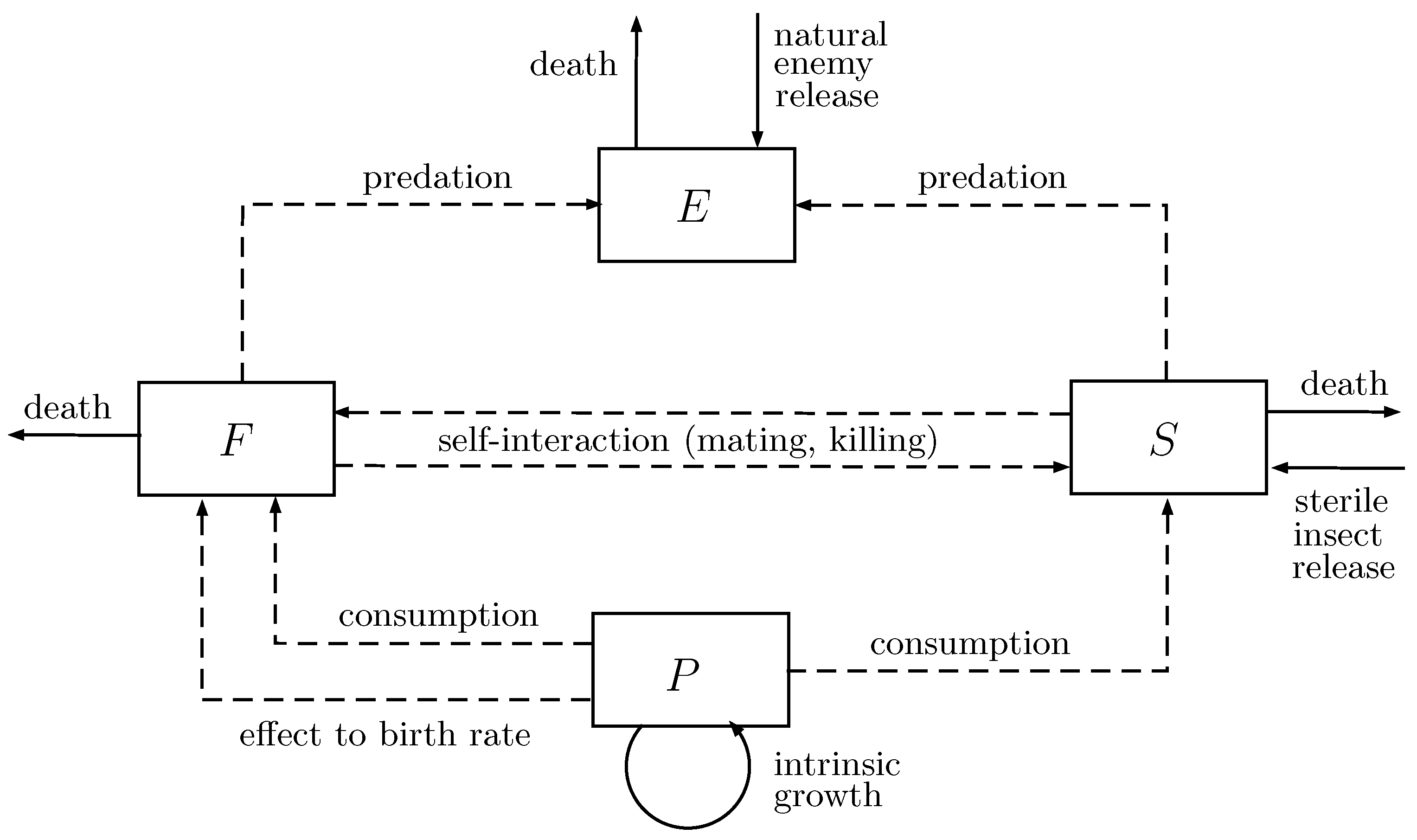
The interactions of plant, pests and natural enemies are distributed into three classes of populations but four state variables. We denote by $P\left(t\right)$ the density of plants at time t, by $F\left(t\right)$ the population of fertile pest insects at time t, by $S\left(t\right)$ the population of (male) sterile pest insects at time t and by $E\left(t\right)$ the population of natural enemies at time t. Male pest insects’ population is not explicitly denoted by a variable but it is intrinsically represented by mating process with fertile insects. In one sense, our model extends the pest control model of [30] by incorporating the existence of natural enemies. Another extension is obviously the optimal control formulation, which will be presented in the next subsection.

3.1. Assumptions

For the sake of simplicity, the complexity of pest control process may be sufficiently adjusted. In model construction, we impose the following assumptions:

• The plant grows logistically with intrinsic growth rate $r_p$ in an environment with carrying capacity k.
• Only pest consumes the plant with consumption rate $a_1$ for fertile insects and $a_2$ for sterile insects. Similar to [39], the plant-pest interaction is following a predator-prey Holling type II function with handling time $c_1$ and $c_2$, and constant of half-saturation m. Thus, response functions of plants consumption by fertile and sterile insects are, respectively, given by $g_F\left(P\right)$ and $g_S\left(P\right)$, where

  $$\begin{array}{ccc}\hfill g_F\left(P\right)& =& \frac{a_{1}P}{m+c_{1}P},\hfill \end{array}$$

  (1)

  $$\begin{array}{ccc}\hfill g_S\left(P\right)& =& \frac{a_{2}P}{m+c_{2}P}.\hfill \end{array}$$

  (2)
• Natural enemies consume both fertile and sterile pests with consumption rate $b_F$ and $b_S$, respectively, following a Holling type II response function.
• Conversion efficiencies of plant consumption by fertile insects and sterile insects are, respectively, given by $e_1$ and $e_2$. Since the number of sterile insects is small, then $e_2$ is also small. Here, we assume $e_2\in [0,1]$. Conversion efficiencies of insect consumption by natural enemies is $e_3$. We also assume $e_3\in [0,1]$. It means that consuming one insect can produce at most one predator.
• No migration activity for the population involved in the model. The recruitment happens only from reproductive process or manual release.
• Introduction of sterile pest insects reduces the birth rate of pest. The intrinsic birth rate is $r_h$, and by the release of sterile pest insects, it decreases to $r_{h}F/(F+S)$. As in [43,44], we further assume that the growth of fertile insect depends on the availability of plant as the food resource. Thus, the pest birth rate r is given by

  $$r=\frac{e_1{a}_{1}P}{m+c_{1}P}\frac{r_{h}F}{1+F+S}.$$

  (3)
• Biological control agents have the same survivability as wild agents. However, there are three causes of pest death: natural cause ($d_F$, $d_S$), self-interaction (${\alpha }_F$, ${\alpha }_S$) and fertile-sterile interaction ($\beta$). Those of natural enemy be denoted by $d_E$ and ${\alpha }_E$.
• Sterile insects are released depending on the population of fertile insects with rate $R_1\left(F\right)$, while natural enemies are introduced depending on the population of fertile and sterile insects with rate $R_2(F,S)$.

A compartmental diagram, which classifies individuals into four different groups of population, is then constructed based on aforementioned assumptions, as depicted in Figure 1. The motions of the population transfer are represented by solid arched lines, while interactions between population are illustrated by dashed lines.

3.2. Mathematical Model

The interdependence among plant, pest insects and natural enemies, as shown in compartmental model in Figure 1, are then formulated in a set of nonlinear ordinary differential equations. This system of equations constitutes as the equations of motion which govern the dynamical transitions.

The plant P grows to provide a supply of certain commodities as well as become a source of food for pests. Its dynamics obey the following equation:

$$\frac{dP}{dt}=r_{p}P\left(1-\frac{P}{k}\right)-\frac{a_{1}P}{m+c_{1}P}F-\frac{a_{2}P}{m+c_{2}P}S.$$

(4)

The first term in the right-hand side of (4) denotes a logistic growth of plant with intrinsic growth rate $r_p$ and under carrying capacity k. The last two terms represent the amount of plant consumed by both fertile and sterile pests, respectively. The intake rates follow the Holling type II functions provided in (1) and (2).

The dynamics of fertile pest insect population F are given by

$$\frac{dF}{dt}=\frac{e_1{a}_{1}P}{m+c_{1}P}\frac{r_{h}F}{1+F+S}F-\frac{b_{F}F}{1+F+S}E-(d_F+{\alpha }_{F}F+\beta S)F,$$

(5)

where the increase in population due to births is expressed by the first term of the right-hand side of (5). Note that the existence of sterile insects S in the denominator provides a negative effect on the growth, i.e., it drops the birth rate. However, this lowering is balanced by the effect of plant ingestion. The population reduction due to predation by natural enemies with rate $b_F$ is stated by the second term, where the intake rate also adheres a Holling type II function. The last terms account the death of fertile pest insects.

The sterile pest insect population S grows by consuming plant and recedes due to predation and death. Additional population is obtained by manually releasing sterile insects into the wild. Thus, we have

$$\frac{dS}{dt}=\frac{e_2{a}_{2}P}{m+c_{2}P}S-(d_S+{\alpha }_{S}S+\beta F)S-\frac{b_{S}S}{1+F+S}E+{\epsilon }_1{u}_1{R}_1\left(F\right).$$

(6)

In (6), $u_1=u_1\left(t\right)$ denotes the control measure of applying SIT. The release rate of sterile pest insect is given by $R_1\left(F\right)$, i.e., it depends on the number of fertile counterparts. This control action is implemented with degree of effectiveness ${\epsilon }_1$.

Similarly, a number of natural enemies can manually be released to prey on pest. The release rate is $R_2(F,S)$, in which it depends on the number of fertile and sterile pest insects. This control action is denoted by $u_2=u_2\left(t\right)$ with degree of effectiveness ${\epsilon }_2$. The state transitions of natural enemies are then represented as

$$\frac{dE}{dt}=\frac{e_3(b_{F}F+b_{S}S)}{1+F+S}E-(d_E+{\alpha }_{E}E)E+{\epsilon }_2{u}_2{R}_2(F,S),$$

(7)

where the first term of the right-hand side of (7) denotes the growth of natural enemy due to food conversion and the second term records the death.

We call (4)–(7) the dynamical system, i.e., a set of equations that describes the dynamics of state variables. We assume that the system satisfies the following initial conditions:

$$P\left(0\right)=P_0,F\left(0\right)=F_0,S\left(0\right)=S_0,E\left(0\right)=E_0,$$

(8)

with initial values $P_0,F_0,S_0,E_0$ being all non-negative, and the following terminal time conditions:

$$P\left(T\right)=P_T,F\left(T\right)=F_T,S\left(T\right)=S_T,E\left(T\right)=E_T,$$

(9)

with terminal values $P_T$, $F_T$, $S_T$, and $E_T$ being all free, and $T>0$ is a fixed finite horizon of control implementation. Conditions (9) will lead to transversality conditions to be satisfied by associated adjoint variables. We also impose bounded control policies:

$$\begin{array}{ccc}& & 0\le u_1\left(t\right)\le {\overline{u}}_1,\hfill \end{array}$$

(10)

$$\begin{array}{ccc}& & 0\le u_2\left(t\right)\le {\overline{u}}_2,\hfill \end{array}$$

(11)

for all $t\in [0,T]$. Upper bounds ${\overline{u}}_1$ in (10) and ${\overline{u}}_2$ in (11) will be determined according to release rates $R_1\left(F\right)$ and $R_2(F,S)$. The set of all admissible control functions is given by

$$\mathbb{U}=\left\{u\left(t\right)\right|u\left(t\right)\in L^{\infty }(0,T),0\le u\left(t\right)\le \overline{u}\},$$

(12)

where $u\left(t\right)={(u_1\left(t\right),u_2\left(t\right))}^{\mathsf{T}}$ and $L^{\infty }$ be the set of all Lebesgue integrable functions.

3.3. Release Rates

The number of released agents is one factors that can influence the effectiveness of control by augmentation. The release rate of biological control agents should be optimally decided as increasing the number of agents released into a wild environment did increase the control cost but did not always lead to effective control of pest insects [29]. To assess the effect of natural enemy and sterile insect release rates on pest suppression mechanism, we consider three different time independent release strategies, namely, constant, proportional and saturating proportional release rates [45].

Constant control rates of sterile insect and natural enemy releases assign $R_1\left(F\right)=1$ and $R_2(F,S)=1$. In this case, the control variables $u_1\left(t\right)$ and $u_2\left(t\right)$ are defined as the number of sterile insects and natural enemies released at time t, respectively, while ${\overline{u}}_1$ and ${\overline{u}}_2$ are defined as the maximum availability of biological agents. By proportional control rates, we consider release rates that proportional to the number of corresponding pest insects. As sterile insects will interact with their fertile counterparts, then we specify $R_1\left(F\right)=F$. Consequently we define $u_1\left(t\right)$ as the portion of sterile insects to be released with respect to the number of fertile insects in the environment, and thus ${\overline{u}}_1=1$ is set. Similarly, since natural enemies will prey on both fertile and sterile insects, then we define $R_2(F,S)=F+S$ and $u_2\left(t\right)$ is the share of natural enemies to be released with respect to the number of whole pest with ${\overline{u}}_2=1$. Saturating proportional rates aim to have proportional rates for small number of populations but become saturated for sufficiently large number of populations. Thus, in this case, we assign $R_1\left(F\right)=F/(1+F)$ and $R_2(F,S)=(F+S)/(1+F+S)$ and define ${\overline{u}}_1$ and ${\overline{u}}_2$ similar to the cases of constant release rate. We summarize the setting of release rates in

Table 1. The release rate strategies.

Release Rate	Sterile Insect	Natural Enemy	Control Upper Bound
Constant	$R_1\left(F\right)=1$	$R_2(F,S)=1$	${\overline{u}}_i\ge 1$
Proportional	$R_1\left(F\right)=F$	$R_2(F,S)=F+S$	${\overline{u}}_i=1$
Saturating proportional	$R_1\left(F\right)=\frac{F}{1+F}$	$R_2(F,S)=\frac{F+S}{1+F+S}$	${\overline{u}}_i\ge 1$

.

3.4. Control Performance Index

Given the system (4)–(7), initial time conditions (8) and terminal time conditions (9), we aim to find the bounded control variables $u_1\left(t\right)$ and $u_2\left(t\right)$ such that they minimize the following performance index:

$$J(u_1\left(t\right),u_2\left(t\right))={\int }_0^T\left(W_{0}F\left(t\right)+W_1{u}_1^2\left(t\right)+W_2{u}_2^2\left(t\right)\right)dt$$

(13)

under the choice of release rate strategies given in Table 1. It is stated in (13) that we want to minimize the population of fertile pests while also keeping the costs of releasing sterile insects and natural enemies low. Here, we assume a quadratic form of control cost application. The coefficients $W_0$, $W_1$ and $W_2$ are balancing weights due to size and importance of the three parts of the control performance criterion. Therefore, the optimal controls $u_1^{*}\left(t\right)$ and $u_2^{*}\left(t\right)$ must be sought such that

$$J(u_1^{*}\left(t\right),u_2^{*}\left(t\right))=\underset{\begin{array}{c}{u}_1\left(t\right),u_2\left(t\right)\in \mathbb{U}\\ t\in [0,T]\end{array}}{min}J(u_1\left(t\right),u_2\left(t\right)),$$

(14)

where the admissible control set $\mathbb{U}$ is given in (12).

4. Analysis of Optimal Control

An optimal control pair $(u_1^{*}\left(t\right),u_2^{*}\left(t\right))$ must satisfy the necessary conditions derived from Pontryagin’s maximum principle [46]. First we have to ensure the existence such a control pair.

4.1. Existence

The existence, nonnegativity and boundedness of solution to model (4)–(7) are presented in the following theorem.

Theorem 1.

Given model (4)–(7) with initial conditions (8). The solutions to this model are positive and bounded.

Proof of Theorem 1.

Let define the total ’population’ N as $N\left(t\right)=P\left(t\right)+F\left(t\right)+S\left(t\right)+E\left(t\right)$, from which we have $\frac{dN}{dt}=\frac{dP}{dt}+\frac{dF}{dt}+\frac{dS}{dt}+\frac{dE}{dt}$. Terms in the right-hand side are then substituted by those of model (4)–(7). After dropping some terms with negative value, by considering that some positive terms are less than one, and by noticing that $u_1,u_2,R_1,R_2$ are all bounded, we may write

$$\frac{dN}{dt}\le r_{p}P\left(1-\frac{P}{k}\right)+\overline{r}F-(d_F+{\alpha }_{F}F)F-d_{S}S-d_{E}E+\overline{R},$$

where $\overline{R}={sup}_{t\in [0,T]}\{{\epsilon }_1{u}_1{R}_1+{\epsilon }_2{u}_2{R}_2\}$ and $\overline{r}=max\left\{\frac{e_1{a}_{1}P}{m+c_{1}P}\frac{r_{h}F}{1+F+S}\right\}$ is the maximum saturation. To strengthen the expression, let us define the following quantities:

$$\begin{array}{cc}\hfill d& =min\{d_F,d_S,d_E\},\hfill \end{array}$$

(15)

$$\begin{array}{cc}\hfill {\theta }_1& =\frac{r_p}{4k}{\left(k+\frac{dk}{r_p}\right)}^2,\hfill \end{array}$$

(16)

$$\begin{array}{cc}\hfill {\theta }_2& =\frac{{\overline{r}}^2}{4{\alpha }_F}.\hfill \end{array}$$

(17)

Then we obtain

$$\frac{dN}{dt}\le -dN-\frac{r_p}{k}{\left(P-\frac{1}{2}\left(k+\frac{dk}{r_p}\right)\right)}^2+{\theta }_1-{\alpha }_F{\left(F-\frac{\overline{r}}{2{\alpha }_F}\right)}^2+{\theta }_2+\overline{R}.$$

Again, by dropping terms with negative value and by assigning $\theta ={\theta }_1+{\theta }_2+\overline{R}$, we have $\frac{dN}{dt}+dN\le \theta$. This differential inequality has the solution

$$0\le N\left(t\right)\le \frac{\theta }{d}+\left(N_0-\frac{\theta }{d}\right)e^{-dt}.$$

This solution is bounded by the steady-state value $\overline{N}=\frac{\theta }{d}$ as time t becomes infinite, meaning that the model is mathematically and ecologically well-posed with bounded state variables. The invariant region $\mathbb{S}$ is then given by

$$\mathbb{S}=\left\{{(P,F,S,E)}^{\mathsf{T}}\in {\mathbb{R}}_{+}^4|0\le P+F+S+E\le \frac{\theta }{d}\right\}.$$

This completes the proof. □

4.2. Necessary Conditions

Pontryagin’s maximum principle transforms the model (4)–(7), performance index (13) and its optimal value (14) into a problem of pointwisely minimizing a Hamiltonian H with respect to control variables $u_1$ and $u_2$. The Hamiltonian is defined as follows:

$$H(X,p,u)=W_{0}F+W_1{u}_1^2+W_2{u}_2^2+p_1{f}_1+p_2{f}_2+p_3{f}_3+p_4{f}_4,$$

(18)

where $X={(P,F,S,E)}^{\mathsf{T}}$ is the vector of state variables, $p_i=p_i\left(t\right)$, for $i=1,2,3,4$, are the adjoint variables, $p={(p_1,p_2,p_3,p_4)}^{\mathsf{T}}$ is the vector of adjoint variables, and $f_i=f_i(X,u)$, for $i=1,2,3,4$, are the right-hand side of model (4)–(7).

Pontryagin’s maximum principle consists of the following requirements:

$$\begin{array}{cc}\hfill \frac{d{X}_i}{dt}& =\frac{\partial H}{\partial p_i},i=1,2,3,4,\hfill \end{array}$$

(19)

$$\begin{array}{cc}\hfill \frac{\partial H}{\partial u_j}& =0,j=1,2,\hfill \end{array}$$

(20)

$$\begin{array}{cc}\hfill \frac{d{p}_i}{dt}& =-\frac{\partial H}{\partial X_i},i=1,2,3,4.\hfill \end{array}$$

(21)

Conditions (19) obviously produce the model (4)–(7), conditions (20) give the optimal controls, and conditions (21) provide the so-called adjoint system. The second and third requirements are presented in the following theorems.

Theorem 2.

The optimal control pair $(u_1^{*},u_2^{*})$ that satisfies (14) is provided by:

$$\begin{array}{cc}\hfill u_1^{*}\left(t\right)& =min\left\{{\overline{u}}_1,max\left\{0,-\frac{{\epsilon }_1}{2W_1}{p}_3\left(t\right)R_1\left(F\right)\right\}\right\},\hfill \end{array}$$

(22)

$$\begin{array}{cc}\hfill u_2^{*}\left(t\right)& =min\left\{{\overline{u}}_2,max\left\{0,-\frac{{\epsilon }_2}{2W_2}{p}_4\left(t\right)R_2(F,S)\right\}\right\},\hfill \end{array}$$

(23)

where $R_1\left(F\right)$ and $R_2(F,S)$ are provided by Table 1.

Proof of Theorem 2.

Application of (20) gives $2W_1{u}_1+{\epsilon }_1{p}_3{R}_1=0$ and $2W_2{u}_2+{\epsilon }_2{p}_4{R}_2=0$, from which we then obtain

$$\begin{array}{cc}\hfill u_1\left(t\right)& =-\frac{{\epsilon }_1}{2W_1}{p}_3\left(t\right)R_1\left(F\right),\hfill \end{array}$$

(24)

$$\begin{array}{cc}\hfill u_2\left(t\right)& =-\frac{{\epsilon }_2}{2W_2}{p}_4\left(t\right)R_2(F,S).\hfill \end{array}$$

(25)

By considering $u_1$ and $u_2$ are bounded as stated, respectively, in (10) and (11), we can rewrite (24) and (25) in the forms of (22) and (23). □

Theorem 2 shows that the optimal controls, i.e., the optimal number of sterile insects and natural enemies should be released, depend explicitly on their release rates.

Theorem 3.

Given the optimal state solution $X^{*}={(P^{*},F^{*},S^{*},E^{*})}^{\mathsf{T}}$ associated with the optimal control pair $u^{*}={(u_1^{*},u_2^{*})}^{\mathsf{T}}$ in (22) and (23), the adjoint variables $p_i(i=1,2,3,4)$ satisfy the following system of differential equations:

$$\frac{d{p}_1}{dt}=\left(p_{1}F-\frac{e_1{r}_h{p}_2{F}^2}{1+F+S}\right)\frac{a_{1}m}{{(m+c_{1}P)}^2}+\frac{a_{2}m(p_1-e_2{p}_3)S}{{(m+c_{2}P)}^2}-r_p{p}_1\left(1-\frac{2P}{k}\right),$$

(26)

$$\begin{array}{cc}\frac{d{p}_2}{dt}=& -W_0+\frac{a_1{p}_{1}P}{m+c_{1}P}+\frac{b_F(p_2-e_3{p}_4)E(1+S)}{1+F+S}+\frac{b_S(e_3{p}_4-p_3)SE}{{(1+F+S)}^2}\hfill \\ & +(p_2+p_3)\beta S+p_2\left(d_F+2{\alpha }_{F}F-\frac{e_1{a}_1{r}_{h}P}{m+c_{1}P}\frac{2F(1+S)+F^2}{{(1+F+S)}^2}\right)\hfill \\ & -p_3{\epsilon }_1{u}_1\frac{\partial R_1}{\partial F}-p_4{\epsilon }_2{u}_2\frac{\partial R_2}{\partial F},\hfill \end{array}$$

(27)

$$\begin{array}{cc}\frac{d{p}_3}{dt}=& \frac{a_2(p_1-e_2{p}_3)P}{m+c_{2}P}+\frac{b_F(e_3{p}_4-p_2)FE}{{(1+F+S)}^2}+\frac{b_S(p_3-e_3{p}_4)E(1+F)}{{(1+F+S)}^2}\hfill \\ & +(p_2-p_3)\beta F+\frac{e_1{a}_1{p}_{2}P}{m+c_{1}P}\frac{r_h{F}^2}{{(1+F+S)}^2}+p_3(d_S+2{\alpha }_{S}S)-p_4{\epsilon }_2{u}_2\frac{\partial R_2}{\partial S},\hfill \end{array}$$

(28)

$$\begin{array}{cc}\hfill \frac{d{p}_4}{dt}& =\frac{b_F(p_2-e_3{p}_4)F+b_S(p_3-e_3{p}_4)S}{1+F+S}+p_4(d_E+2{\alpha }_{E}E),\hfill \end{array}$$

(29)

with transversality conditions

$$p_i\left(T\right)=0,i=1,2,3,4.$$

(30)

Proof of Theorem 3.

Adjoint system (26)–(29) can be obtained by applying (21). The transversality conditions (30) are consequences of having free terminal time conditions given in (9). □

As in the case of dynamical system and optimal controls, differential Equations (27) and (28) in adjoint system of Theorem 3 will also switch according to the selected release strategy. In these equations, the following switching functions are employed:

$$\begin{array}{cc}\hfill \frac{\partial R_1}{\partial F}& =\left\{\begin{array}{ccc}0\hfill & ;\hfill & \mathrm{for}\mathrm{constant}\mathrm{release}\mathrm{rate}\hfill \\ 1\hfill & ;\hfill & \mathrm{for}\mathrm{proportional}\mathrm{release}\mathrm{rate}\hfill \\ \frac{1}{{(1+F)}^2}\hfill & ;\hfill & \mathrm{for}\mathrm{saturating}\mathrm{proportional}\mathrm{release}\mathrm{rate},\hfill \end{array}\right.\hfill \end{array}$$

(31)

$$\begin{array}{cc}\hfill \frac{\partial R_2}{\partial F}=\frac{\partial R_2}{\partial S}& =\left\{\begin{array}{ccc}0\hfill & ;\hfill & \mathrm{for}\mathrm{constant}\mathrm{release}\mathrm{rate}\hfill \\ 1\hfill & ;\hfill & \mathrm{for}\mathrm{proportional}\mathrm{release}\mathrm{rate}\hfill \\ \frac{1}{{(1+F+S)}^2}\hfill & ;\hfill & \mathrm{for}\mathrm{saturating}\mathrm{proportional}\mathrm{release}\mathrm{rate}.\hfill \end{array}\right.\hfill \end{array}$$

(32)

5. Illustrative Example

In this section, we present an illustrative example to clarify the modeling approach. We consider an interaction between rice plant (Oryza sativa) and brown planthopper (Nilaparvata lugens) as pest insect. To control the pest population, in this growing environment we also release a number of (male) sterile brown planthoppers (SIT) and Asian ladybeetles (Harmonia axyridis) as natural enemy.

As mentioned previously, there are three release strategies available for sterile insects and natural enemies, namely, constant (C), proportional (P) and saturating proportional (S). We compare control combinations with the case where no single control implemented, i.e., $u_1\left(t\right)=u_2\left(t\right)=0$ for all $t\in [0,T]$. Thus, we have nine control combinations: C-C, C-P, C-S, P-C, P-P, P-S, S-C, S-P, and S-S, where C-C means constant release rate for SIT and constant release rate for natural enemies, etc. For constant and saturating proportional release strategies we set ${\overline{u}}_1={\overline{u}}_2=10$ and for proportional release strategies we set ${\overline{u}}_1={\overline{u}}_2=1$. Initially, we consider an environment with plenty of pests but few number of natural enemies, i.e., we specify $P_0=300$, $F_0=50$, $S_0=3$, and $E_0=2$. In the control objective, we emphasize on the pest density suppression. Thus, we set the weights $W_0=100$ and $W_1=W_2=1$. The value of other parameters can be found in

Table 2. The value of parameters.

Parameter	Description	Value	Unit
$P_0$	initial plant density	300	g/unit area
$F_0$	initial population of fertile insects	50	individual
$S_0$	initial population of sterile insects	3	individual
$E_0$	initial population of natural enemies	2	individual
$r_p$	intrinsic growth rate of plant	$0.15$	g/unit area/day
k	environment carrying capacity	1000	g/unit area
$r_h$	intrinsic birth rate of fertile insects	$1.25$	insect/day
$a_1$	plant consumption rate by fertile insects	$0.4515$	g/day
$a_2$	plant consumption rate by sterile insects	$0.7$	g/day
$c_1$	handling time by fertile insects	1	day
$c_2$	handling time by sterile insects	1	day
m	constant of half saturation	$0.8$	per unit area
$b_F$	fertile insect consumption rate by predator	$0.75$	insect/day
$b_S$	sterile insect consumption rate by predator	$0.75$	insect/day
$d_F$	death rate of fertile insect	$0.0238$	insect/day
$d_S$	death rate of sterile insect	$0.0238$	insect/day
$d_E$	death rate of natural enemy	$0.0140$	insect/day
${\alpha }_F$	death rate of fertile insect due to fertile-fertile interaction	$0.0714$	insect/day
${\alpha }_S$	death rate of fertile insect due to sterile-sterile interaction	$0.0714$	insect/day
$\beta$	death rate of fertile insect due to fertile-sterile interaction	$0.0714$	insect/day
${\alpha }_E$	death rate of natural enemy due to self-interaction	$0.0704$	insect/day
$e_1$	plant-to-fertile insect conversion factor	$9.272$	insect/unit area/day
$e_2$	plant-to-sterile insect conversion factor	$0.0029$	insect/unit area/day
$e_3$	insect-to-natural enemy conversion factor	1	insect/day
${\epsilon }_1$	effectiveness of control using SIT	$70\%$	-
${\epsilon }_2$	effectiveness of control using natural enemy release	$85\%$	-
$W_0$	weight showing the importance of pest density suppression	100	-
$W_1$	weight showing the importance of control effort by SIT	1	-
$W_2$	weight showing the importance of control effort by natural enemy	1	-
T	control period	15	day

. Most of parameters values used in the simulation are taken from [47,48,49,50,51].

5.1. Numerical Methods

The optimality conditions of a control problem come from Pontryagin’s maximum principle and consist of state system (4)–(7), optimal controls (22) and (23), and adjoint system (26)–(29). From numerical computation point of view, this control problem is challenging since the state system X has initial values (8) but the adjoint system p possesses terminal values (30). One advantage we have is that the determination of optimal solution $X^{*}$ is independent of p. We thus use sweep method [52], which consists of forward and backward fourth order Runge–Kutta algorithms, to concurrently solve this mixed boundary values problem. The outline of this approach is as follows. Let the vector approximations for state variable X, adjoint variable p, and control variable u be denoted by $\tilde{X}$, $\tilde{p}$, and $\tilde{u}$, respectively.

• Set the initial values of state variable ${\tilde{X}}_0$, adjoint variable ${\tilde{p}}_0$, and control variable ${\tilde{u}}_0$ as well as tolerance level of convergence $\epsilon$.
• Using initial value $X\left(0\right)=X_0$, solve X forwardly according to (4)–(7) and make updating $\tilde{X}(i+1)=\tilde{X}\left(i\right)+hn$, where h is step-size and n is the weighted average slope of the fourth order Runge–Kutta algorithm.
• Using terminal value $p\left(T\right)=0$ and state variable $\tilde{X}$ obtained from previous step, solve p backwardly according to (26)–(29) and make updating $\tilde{p}\left(j\right)=\tilde{p}(j+1)-hn$.
• Using X and p obtained from previous steps, calculate $\tilde{u}$ according to control laws (22) and (23). Update the value of control variables as the average between current and updated values.
• Return to step 2 until convergence is reached: ${max}_i\parallel {\tilde{u}}_i^{\mathrm{new}}-{\tilde{u}}_i^{\mathrm{old}}\parallel \le \epsilon$.

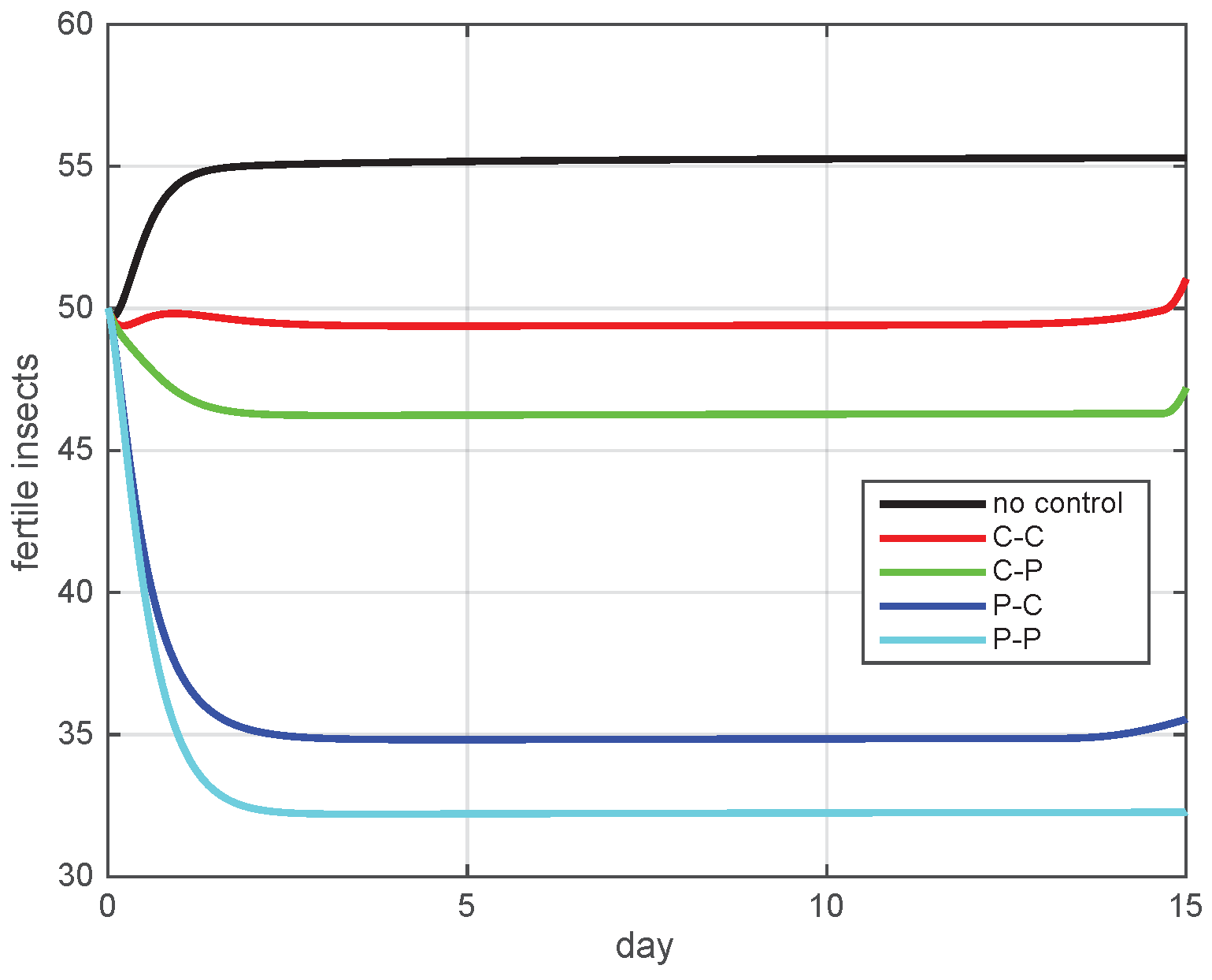
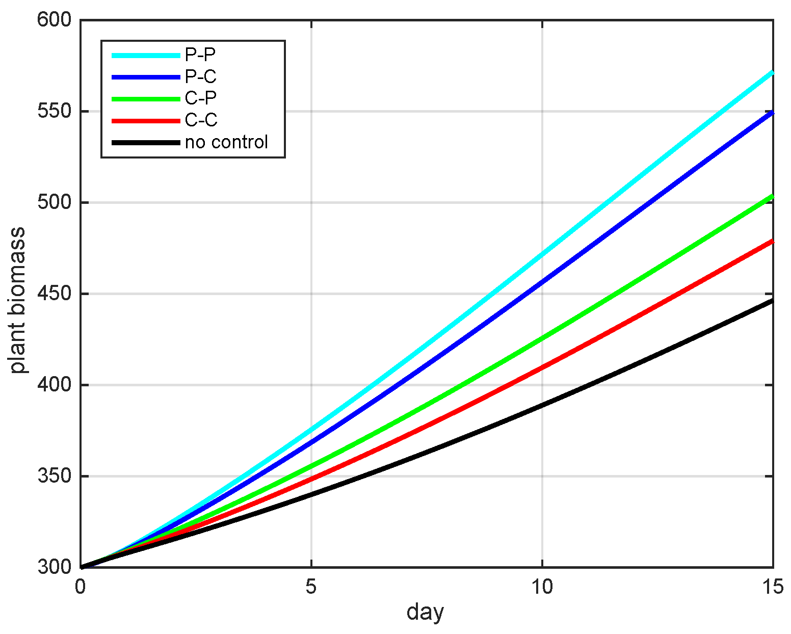
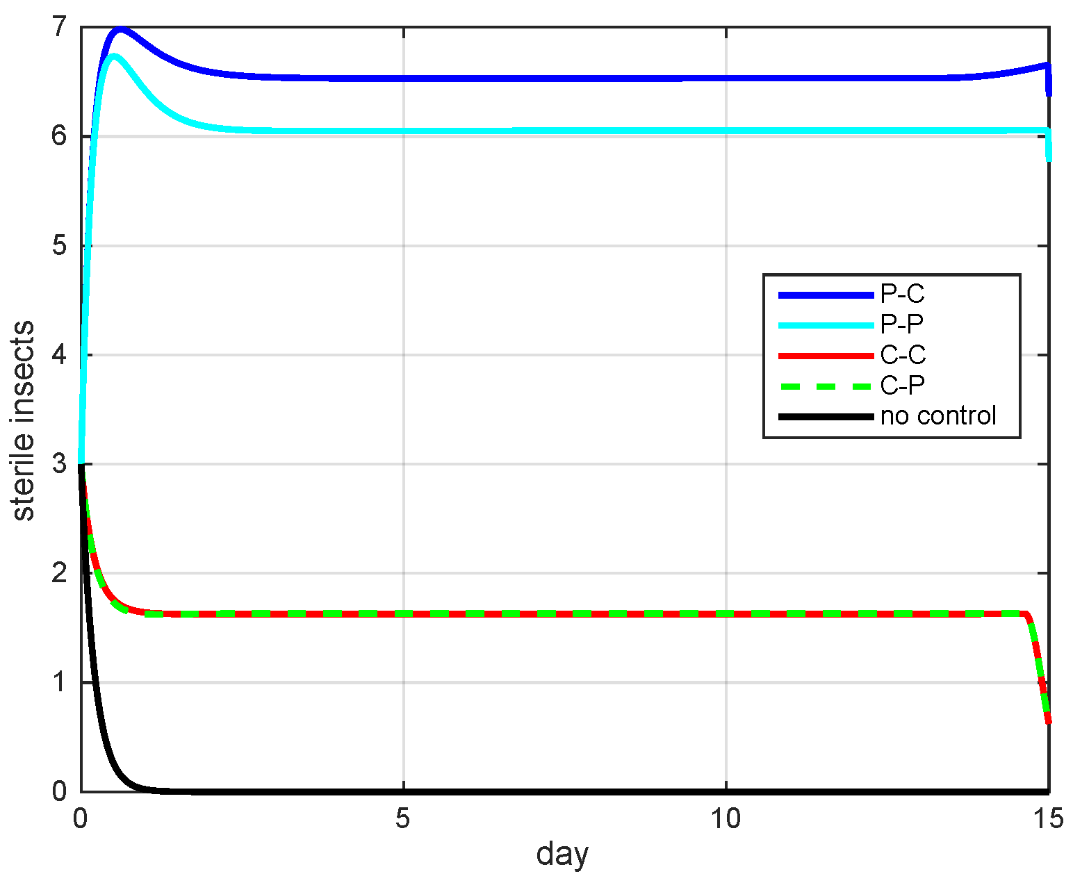
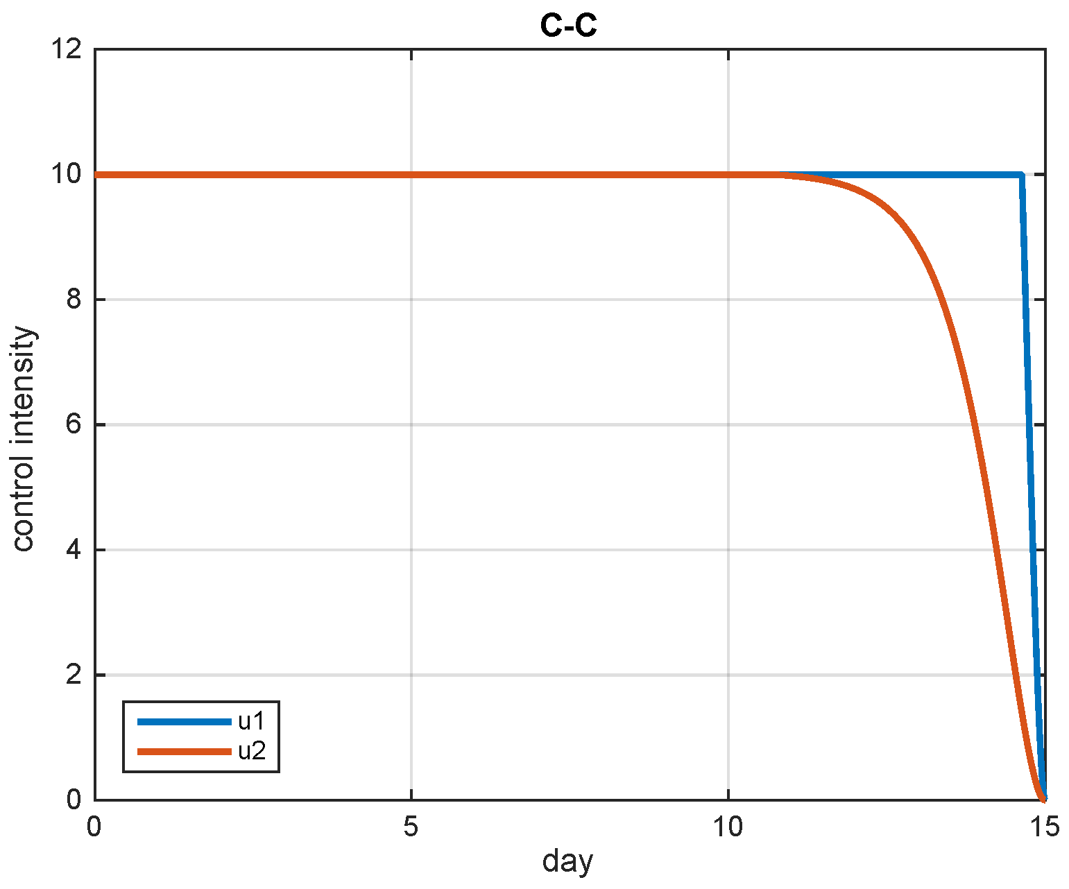
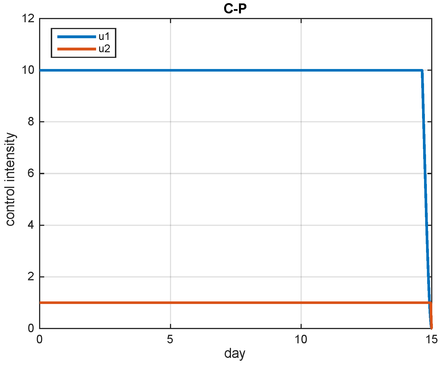
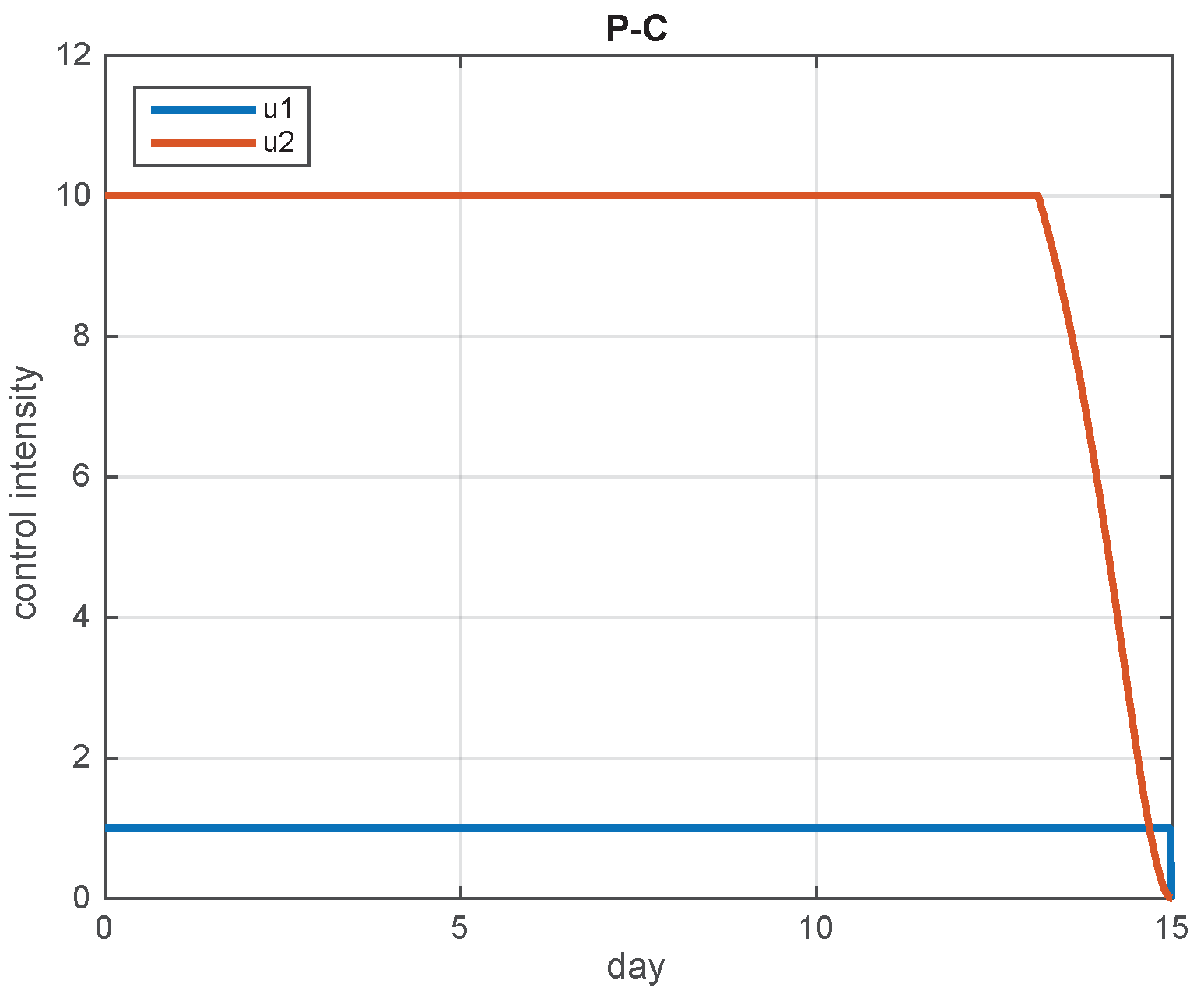
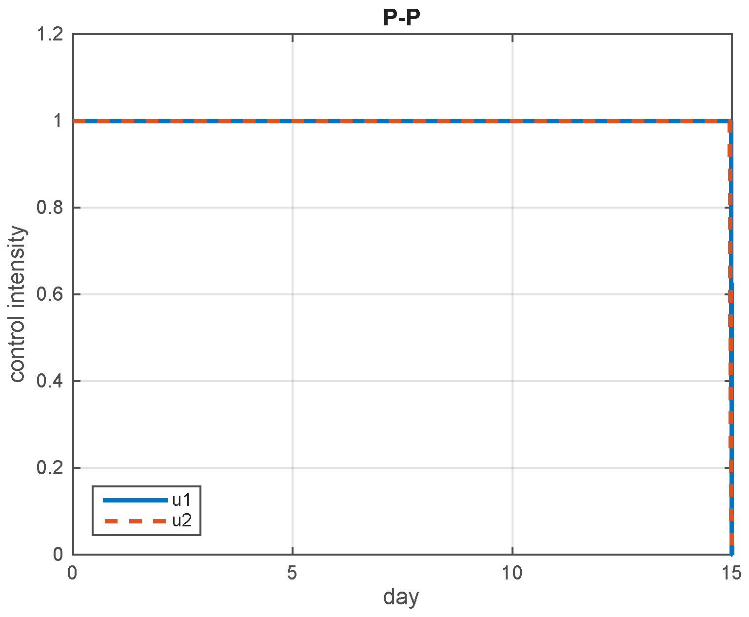
5.2. Simulation Results

Our preliminary analysis reveals that some control combinations, i.e., some release rate strategies, show identical simulation results. We found that strategies C-C, C-S, S-C, and S-S perform identical control behaviors. Likewise with P-C and P-S, and S-P and C-P. It can be understood that strategy of saturating proportional release rate (S) mimics the control behavior of constant release rate, particulary for larger population size, as $\frac{F}{1+F}$ and $\frac{F+S}{1+F+S}$ tend to 1 for sufficiently large F and/or S. Therefore, in this part we only present simulation results with different control dynamics, i.e., C-C, C-P, P-C, and P-P.

Figure 2 and Figure 3 depict the fertile pest insect population (brown planthopper) and the plant density (rice) dynamics under all control scenarios. It can be seen in Figure 2 that, without control action, the number of fertile planthoppers will increase from 50 to 55 and it becomes in steady state from $t=2$. Under control actions, the planthopper population is successfully suppressed with strategy P-P provides the most effect as it reduces to about 33, followed by strategy P-C (35), strategy C-P (about 47), and strategy C-C provides the least (about 49). Even though the rice plant is being attacked by pests and we perform no control strategy, the rice plant biomass can still grow. However, the growth is accelerated when a control action is imposed, with strategy P-P contributes the most effect and strategy C-C the least (see Figure 3).

In Figure 4 and Figure 5, we present the dynamics of sterile brown planthopper and Asian ladybeetle as natural enemies. Initially, the number of sterile planthoppers is 3 and that of ladybeetles is 2. Without intervention, the sterile planthoppers and ladybeetles are extinct, causing an increase in fertile planthoppers as confirmed in Figure 2. However, control actions in the form of SIT and ladybeetle augmentation can prevent these two populations from extinction. It is shown in Figure 4 that strategies P-C and P-P increase steadily the population of sterile planthoppers to around 6–7, but strategies C-C and C-P can also steadily preserve the population even though the size is below the initial value. Figure 5 shows that strategies C-P and P-P can steadily raise the population of ladybeetles to about 22 and 20, respectively. While strategies C-C and P-C can steadily increase the population of natural enemies to about 9. These facts confirm that the release of sterile brown planthoppers and Asian ladybeetles can effectively hamper the growth of pests.

Figure 6, Figure 7, Figure 8 and Figure 9 illustrate the optimal implementation of control actions. It can be seen immediately that under both constant and proportional rates, brown planthoppers must be released at the maximum level. While the Asian ladybeetles are released at maximum capacity only when proportional rates are applied. This means control measure in the form of SIT is considered more forceful in controlling pests.

5.3. The Most Cost-Effective Strategy

If the evaluation of control actions is carried out based on the reduction of the pest population, then strategy P-P is the best. In addition, if the assessment is undertaken based on increasing plant biomass, then again strategy P-P is the most successful. However, there are control costs must be paid in its implementation. Recall that the application of SIT with proportional release rate is given by ${\epsilon }_1{u}_1\left(t\right)F\left(t\right)$, where $0\le u\left(t\right)\le 1$ for all $t\in [0,T]$. If SIT is implemented at maximum capacity, i.e., $u\left(t\right)=1$, then the number of sterile planthoppers released is exactly the same as the number of fertile planthoppers. In the case of constant release rate, the number of sterile planthoppers released does not exceed 10 all the time.

To fairly compare all four strategies, we perform a cost effectiveness analysis (CEA) by considering two metrics relating to cost-effectiveness, namely, the incremental cost-effectiveness ratio (ICER) and the average cost effectiveness ratio (ACER). ICER measures the incremental cost per incremental benefit [53], while ACER calculates the ratio between cost and benefit. The benefit of strategy i, denoted by $B_i$ is defined as the difference in the total number of averted pests through this strategy:

$$B_i={\int }_0^T(F^0\left(t\right)-F^i\left(t\right))dt,$$

(33)

where $F^i\left(t\right)$ is the number of fertile pest insects at time t using strategy i, where $i\in \left\{\mathrm{C}\text{-}\mathrm{C},\mathrm{C}\text{-}\mathrm{P},\mathrm{P}\text{-}\mathrm{C},\mathrm{P}\text{-}\mathrm{P}\right\}$, and $F^0\left(t\right)$ is the number of fertile pest insects with no control application. The cost of strategy i, denoted by $C_i$, is defined as the total operational cost of releasing sterile insects and natural enemies using this strategy:

$$C_i={\int }_0^T(u_1\left(t\right)R_1^i\left(F\right)+u_2\left(t\right)R_2^i(F,S))dt,$$

(34)

where $R_1^i\left(F\right)$ and $R_2^i(F,S)$, respectively, are release rates of sterile insects and natural enemies using strategy i. In calculating $C_i$, we assume the costs of releasing one sterile insect or one natural enemy are unity. The ACER and ICER are then formulated as

$$\begin{array}{cc}\hfill {\mathrm{ACER}}_i& =\frac{C_i}{B_i},\hfill \end{array}$$

(35)

$$\begin{array}{cc}\hfill {\mathrm{ICER}}_i& =\frac{C_i-C_{i-1}}{B_i-B_{i-1}}.\hfill \end{array}$$

(36)

Table 3. The cost effectiveness analysis.

i	Strategy	Benefit	Cost	ACER	ICER	ICER
0	No control	0	0	-	-	-
1	C-C	$82.6622$	$286.7953$	$3.4695$	$3.4695$	ed
2	C-P	$128.6366$	$867.0948$	$6.7407$	d	d
3	P-C	$293.3255$	$671.7646$	$2.2902$	$-1.1861$	$2.2902$
4	P-P	$331.6253$	$1076.0697$	$3.2448$	$10.5563$	$3.2448$

d: dominated, ed: extendedly dominated.

, which is arranged in ascending order with respect to benefit, presents the calculation of ACER and ICER using (35) and (36). From this table we can see that strategy C-C provides the smallest benefit and lowest cost, while strategy P-P gives the largest benefit and highest cost. Based on ACER, strategy P-C is the most cost effective strategy as it has the smallest score. In the first step of ICER calculation, strategy C-P is immediately dominated by strategy P-C as it produces smaller benefit but higher cost. In the second step, strategy C-C is extendedly dominated by strategy P-C as it has bigger ICER score, and thus ruled out. The remaining two strategies P-C and P-P are compared by calculating their ICERs with respect to no control strategy, i.e., their ACERs. It can be concluded from its smaller ACER/ICER score that strategy P-C is the most cost-effective strategy.

The implementation of strategy P-C as the most cost-effective strategy in controlling brown planthopper is as follows. Firstly, sterile planthoppers should be proportionally released with respect to the number of fertile brown planthoppers. This control action should be maintained at maximum intensity until the end of the control period. In other words, sterile planthoppers should be released as many as fertile planthoppers in the field for fifteen days as illustrated in Figure 8. Secondly, ladybeetles as natural enemies of planthoppers should be released at constant rate of ten per day. This rate should be continued until day thirteen and then quickly reduced to the end of control period. From Figure 2 and Figure 3, it can be calculated that strategy P-C can suppress the pest population by 35 percent and thus improve the plant density by 13 percent.

6. Conclusions

We have proposed a simple analytical model of pest control formulated in a system of ordinary nonlinear differential equations, which governs the dynamical interaction between plant and pest populations. This model is furnished with two control instruments, namely, the release of sterile pest insects (SIT) and the release of predators as natural enemies. Thus, the model consists of four classes of population: plant, fertile insect, sterile insect, and natural enemy. The model is also featured in such a way it allows the use of different release rates of sterile insects and natural enemies.

We have examined the effects of constant, proportional, and saturating proportional release rates on the control performance, where the objective functional of the control problem is to minimize the size of fertile pest insect population jointly with the control efforts. Pontryagin maximum principle has been employed in derivation of necessary optimality conditions, and forward–backward sweep method has been utilized in presenting the numerical solution. In an environment populated by rice plant, brown planthopper as pest, and Asian ladybeetle as predator, it has been revealed that the rate of release plays a significant role in achieving control objectives. It has also been proved that a control strategy consisting of releasing sterile insects with proportional rate and simultaneously natural enemies with constant rate is the most cost effective. Compared to the release of natural enemies, SIT is proved to be the more powerful control measure as it should be implemented at maximal intensity for contributing optimal effect in suppressing pests.

References

1. Savary, S.; Willocquet, L.; Pethybridge, S.J.; Esker, P.; McRoberts, N.; Nelson, A. The global burden of pathogens and pests on major food crops. Nat. Ecol. Evol. 2019, 3, 430–439. [Google Scholar] [CrossRef] [PubMed]
2. Skendzic, S.; Zovko, M.; Zivkovic, I.P.; Lesic, V.; Lemic, D. The impact of climate change on agricultural insect pests. Insects 2021, 12, 440. [Google Scholar] [CrossRef] [PubMed]
3. Deutsch, C.A.; Tewksbury, J.J.; Tigchelaar, M.; Battisti, D.S.; Merrill, S.C.; Huey, R.B.; Naylor, R.L. Increase in crop losses to insect pests in a warming climate. Science 2018, 361, 916–919. [Google Scholar] [CrossRef] [PubMed] [Green Version]
4. IPPC Secretariat. Scientific Review of the Impact of Climate Change on Plant Pests—A Global Challenge to Prevent and Mitigate Plant Pest Risks in Agriculture, Forestry and Ecosystems; FAO: Rome, Italy, 2021. [Google Scholar] [CrossRef]
5. Abrol, D.P. Integrated Pest Management: Current Concepts and Ecological Perspective; Elsevier: Oxford, UK, 2014. [Google Scholar] [CrossRef] [Green Version]
6. Lopez, O.; Fernandez-Bolanos, J. Green Trends in Insect Control; RSC Publishing: Cambridge, UK, 2011. [Google Scholar] [CrossRef]
7. Liang, Y.; Luo, M.; Fu, X.; Zheng, L.; Wei, H. Mating disruption of Chilo suppressalis from sex pheromone of another pyralid rice pest Cnaphalocrocis medinalis (Lepidoptera: Pyralidae). J. Insect Sci. 2020, 20, 1–8. [Google Scholar] [CrossRef] [PubMed]
8. Luo, Z.; Magsi, F.H.; Li, Z.; Cai, X.; Bian, L.; Liu, Y.; Xin, Z.; Xiu, C.; Chen, Z. Development and evaluation of sex pheromone mass trapping technology for Ectropis grisescens: A potential Integrated Pest Management strategy. Insects 2020, 11, 15. [Google Scholar] [CrossRef] [Green Version]
9. Bourtzis, K.; Vreysen, M.J.B. Sterile Insect Technique (SIT) and its applications. Insects 2021, 12, 638. [Google Scholar] [CrossRef]
10. Horrocks, K.J.; Avila, G.A.; Holwell, G.I.; Suckling, D.M. Irradiation-induced sterility in an egg parasitoid and possible implications for the use of biological control in insect eradication. Sci. Rep. 2021, 11, 12326. [Google Scholar] [CrossRef] [PubMed]
11. Blomme, G.; Ocimati, W.; Sivirihauma, C.; Vutseme, L.; Mariamu, B.; Kamira, M.; van Schagen, B.; Ekboir, J.; Ntamwira, J. A control package revolving around the removal of single diseased banana stems is effective for the restoration of Xanthomonas wilt infected fields. Eur. J. Plant Pathol. 2017, 149, 385–400. [Google Scholar] [CrossRef]
12. Hajek, A. Natural Enemies: An Introduction to Biological Control; Cambridge University Press: New York, NY, USA, 2004. [Google Scholar]
13. Van Driesche, R.G.; Abell, K. Classical and augmentative biological control. Encycl. Ecol. 2008, 575–582. [Google Scholar] [CrossRef]
14. Horrocks, K.J.; Avila, G.A.; Holwell, G.I.; Suckling, D.M. Integrating sterile insect technique with the release of sterile classical biocontrol agents for eradication: Is the Kamikaze Wasp Technique feasible? BioControl 2020, 65, 257–271. [Google Scholar] [CrossRef]
15. Lu, M.-C.; Chen, H.-R.; Wu, Y.-H. Current status and future perspectives on natural enemies for pest control in Taiwan. Biocontrol Sci. Technol. 2018, 28, 953–960. [Google Scholar] [CrossRef]
16. Martin, E.A.; Reineking, B.; Seo, B.; Steffan-Dewenter, I. Natural enemy interactions constrain pest control in complex agricultural landscapes. Proc. Natl. Acad. Sci. USA 2013, 110, 5534–5539. [Google Scholar] [CrossRef] [PubMed] [Green Version]
17. Perez-Alvarez, R.; Nault, B.A.; Poveda, K. Effectiveness of augmentative biological control depends on landscape context. Sci. Rep. 2019, 9, 8664. [Google Scholar] [CrossRef] [PubMed] [Green Version]
18. Colombo, R.M.; Rossi, E. A modeling framework for biological pest control. Math. Biosci. Eng. 2020, 17, 1413–1427. [Google Scholar] [CrossRef]
19. Yadav, S.; Kumar, V. Study of a prey–predator model with preventing crop pest using natural enemies and control. AIP Conf. Proc. 2021, 2336, 020002. [Google Scholar] [CrossRef]
20. Kumar, S.; Ahmad, S.; Siddiqi, M.I.; Raza, K. Mathematical model for plant-insect interaction with dynamic response to PAD4-BIK1 interaction and effect of BIK1 inhibition. BioSystems 2019, 175, 11–23. [Google Scholar] [CrossRef]
21. Wan, N.F.; Ji, X.Y.; Jiang, J.X.; Li, B. A modelling methodology to assess the effect of insect pest control on agro-ecosystems. Sci. Rep. 2015, 5, 9727. [Google Scholar] [CrossRef] [Green Version]
22. Sassu, F.; Nikolouli, K.; Caravantes, S.; Taret, G.; Pereira, R.; Vreysen, M.J.B.; Stauffer, C.; Caceres, C. Mass-rearing of Drosophila suzukii for Sterile Insect Technique application: Evaluation of two oviposition systems. Insects 2019, 10, 448. [Google Scholar] [CrossRef] [Green Version]
23. Liu, Q.-X.; Su, Z.-P.; Liu, H.-H.; Lu, S.-P.; Ma, B.; Zhao, Y.; Hou, Y.-M.; Shi, Z.-H. The Effect of gut bacteria on the physiology of red palm weevil, Rhynchophorus ferrugineus Olivier and their potential for the control of this pest. Insects 2021, 12, 594. [Google Scholar] [CrossRef]
24. Yan, Y.; Williamson, M.E.; Scott, M.J. Using moderate transgene expression to improve the genetic sexing system of the Australian sheep blow fly Lucilia cuprina. Insects 2020, 11, 797. [Google Scholar] [CrossRef]
25. Gato, R.; Menendez, Z.; Prieto, E.; Argiles, R.; Rodriguez, M.; Baldoquin, W.; Hernandez, Y.; Perez, D.; Anaya, J.; Fuentes, I.; et al. Sterile Insect Technique: Successful suppression of an Aedes aegypti field population in Cuba. Insects 2021, 12, 469. [Google Scholar] [CrossRef]
26. Patinvoh, R.; Susu, A. Mathematical modelling of sterile insect technology for mosquito control. Adv. Entomol. 2014, 2, 180–193. [Google Scholar] [CrossRef] [Green Version]
27. Knipling, E.F. The Basic Principles of Insect Population Suppression and Management; U.S. Department of Agriculture: Washington, DC, USA, 1979.
28. Barclay, H.J. Models for pest control: Complementary effects of periodic releases of sterile pests and parasitoids. Theor. Popul. Biol. 1987, 32, 76–89. [Google Scholar] [CrossRef]
29. Crowder, D.W. Impact of release rates on the effectiveness of augmentative biological control agents. J. Insect Sci. 2007, 7, 15. [Google Scholar] [CrossRef] [PubMed]
30. Bhattacharyya, R.; Mukhopadhyay, B. Mathematical study of a pest control model incorporating sterile insect technique. J. Nat. Resour. Model. 2014, 27, 61–79. [Google Scholar] [CrossRef]
31. Fitri, I.R.; Hanum, F.; Kusnanto, A.; Bakhtiar, T. Optimal pest control strategies with cost-effectiveness analysis. Sci. World J. 2021, 2021, 6630193. [Google Scholar] [CrossRef]
32. Sun, K.; Zhang, T.; Tian, Y. Dynamics analysis and control optimization of a pest management predator-prey model with an integrated control strategy. Appl. Math. Comput. 2017, 292, 253–271. [Google Scholar] [CrossRef]
33. Yu, T.; Tian, Y.; Guo, H.; Song, X. Dynamical analysis of an integrated pest management predator-prey model with weak Allee effect. J. Biol. Dyn. 2019, 13, 218–244. [Google Scholar] [CrossRef]
34. Huang, L.; Chen, X.; Tan, X.; Chen, X.; Liu, X. A stochastic predator-prey model for integrated pest management. Adv. Diff. Equ. 2019, 2019, 360. [Google Scholar] [CrossRef] [Green Version]
35. Mandal, D.S.; Samanta, S.; Alzahrani, A.K.; Chattopadhyay, J. Study of a predator-prey model with pest management perspective. J. Biol. Syst. 2019, 27, 309–336. [Google Scholar] [CrossRef]
36. Mandal, D.S.; Chekroun, A.; Samanta, S.; Chattopadhyay, J. A mathematical study of a crop-pest-natural enemy model with Z-type control. Math. Comput. Simul. 2021, 187, 468–488. [Google Scholar] [CrossRef]
37. Tian, Y.; Zhang, T.; Sun, K. Dynamics analysis of a pest management prey–predator model by means of interval state monitoring and control. Nonlinear Anal. Hybrid Syst. 2017, 23, 122–141. [Google Scholar] [CrossRef]
38. Mathur, K.S. An eco-epidemic pest-natural enemy SI model in two patchy habitat with impulsive effect. Int. J. Appl. Comput. Math. 2016, 3, 2671–2685. [Google Scholar] [CrossRef]
39. Wang, X.; Tian, Y.; Tang, S. A Holling type II pest and natural enemy model with density dependent IPM strategy. Math. Probl. Eng. 2017, 2017, 8683207. [Google Scholar] [CrossRef] [Green Version]
40. Li, C.; Tang, S. The effects of timing of pulse spraying and releasing periods on dynamics of generalized predator-prey model. Int. J. Biomath. 2012, 5, 1250012. [Google Scholar] [CrossRef]
41. Fister, R.K.; McCarthy, M.L.; Oppenheimer, S.F.; Collins, C. Optimal control of insects through sterile insect release and habitat modification. Math. Biosci. 2013, 244, 201–212. [Google Scholar] [CrossRef]
42. Barclay, H.J. Mathematical models for the use of sterile insects. In Sterile Insect Technique. Principles and Practice in Area-Wide Integrated Pest Management, 2nd ed.; Dyck, V.A., Hendrichs, J., Robinson, A., Eds.; CRC Press: Boca Raton, FL, USA, 2021; pp. 201–244. [Google Scholar] [CrossRef]
43. Dahlin, I.; Ninkovic, V. Aphid performance and population development on their host plants is affected by weed-crop interactions. J. Appl. Ecol. 2013, 50, 1281–1288. [Google Scholar] [CrossRef]
44. Dixon, A.F.G. Structure of aphid populations. Ann. Rev. Entomol. 1985, 30, 155–174. [Google Scholar] [CrossRef]
45. Dhahbi, A.B.; Chargui, Y.; Boulaaras, S.M.; Khalifa, S.B.; Koko, W.; Alresheedi, F. Mathematical Modelling of the Sterile Insect Technique Using Different Release Strategies. Math. Probl. Eng. 2020, 2020, 8896566. [Google Scholar] [CrossRef]
46. Pontryagin, L.S.; Boltyanskii, V.G.; Gamkrelidze, R.V.; Mishchenko, E.F. The Mathematical Theory of Optimal Process; Gordon & Breach: New York, NY, USA, 1986. [Google Scholar]
47. Ali, A.; Memon, S.A.; Mastoi, A.H.; Narejo, M.N.; Azizullah, A.; Afzal, M.; Ahmed, S. Biology and feeding potential of ladybird beetle (Coccinella septempunctata) against different species of aphids. Sci. Int. 2017, 29, 1261–1263. [Google Scholar]
48. Win, S.S.; Muhamad, R.; Ahmad, Z.A.M.; Adam, N.A. Life table and population parameters of Nilaparvata lugens Stal. (Homoptera: Delphacidae) on rice. Trop. Life Sci. Res. 2011, 22, 25–35. [Google Scholar] [PubMed]
49. Sardar, M.; Khatun, M.R.; Islam, K.S.; Haque, M.T.; Das, G. Potentiality of light source and predator for controlling brown planthopper. Progress. Agric. 2019, 30, 275–281. [Google Scholar] [CrossRef] [Green Version]
50. Limohpasmanee, W.; Kongratarpon, T.; Tannarin, T. The effect of gamma radiation on sterility and mating ability of brown planthopper, Nilaparvata lugens (Stal) in field cage. J. Phys. Conf. Ser. 2017, 860, 012004. [Google Scholar] [CrossRef] [Green Version]
51. Riddick, E.W. Identification of conditions for successful aphid control by ladybirds in greenhouses. Insects 2017, 8, 38. [Google Scholar] [CrossRef] [PubMed] [Green Version]
52. Lenhart, S.; Workman, J.T. Optimal Control Applied to Biological Models; CRC Press: Boca Raton, FL, USA, 2007. [Google Scholar]
53. Paulden, M. Calculating and interpreting ICERs and net benefit. Pharmacoeconomics 2020, 38, 785–807. [Google Scholar] [CrossRef] [PubMed]
Figure 1. Compartmental model of pest control with natural enemies and sterile insects releases.
Mathematics 10 00883 g001
Figure 2. Fertile pest insect population.
Mathematics 10 00883 g002
Figure 3. Plant density.
Mathematics 10 00883 g003
Figure 4. Sterile pest insect population.
Mathematics 10 00883 g004
Figure 5. Natural enemy population.
Mathematics 10 00883 g005
Figure 6. Optimal control under C-C strategy.
Mathematics 10 00883 g006
Figure 7. Optimal control under C-P strategy.
Mathematics 10 00883 g007
Figure 8. Optimal control under P-C strategy.
Mathematics 10 00883 g008
Figure 9. Optimal control under P-P strategy.
Mathematics 10 00883 g009