
SVseg: Stacked Sparse Autoencoder-Based Patch Classification Modeling for Vertebrae Segmentation
by
 , , ,
, , ,
Syed Furqan Qadri
1,2 ,
,
Linlin Shen
1,2,*,
Mubashir Ahmad
3,
Salman Qadri
4,
Syeda Shamaila Zareen
5 and
Muhammad Azeem Akbar
6 1
Computer Vision Institute, College of Computer Science and Software Engineering, Shenzhen University, Shenzhen 518060, China
2
AI Research Center for Medical Image Analysis and Diagnosis, Shenzhen University, Shenzhen 518060, China
3
Department of Computer Science and IT, The University of Lahore, Sargodha Campus, Sargodha 40100, Pakistan
4
Department of Computer Science, MNS-University of Agriculture, Multan 60650, Pakistan
5
Faculty of Information Technology, Beijing University of Technology, Beijing 100124, China
6
Department of Information Technology, Lappeenranta University of Technology, 53851 Lappeenranta, Finland
*
Author to whom correspondence should be addressed.
Mathematics 2022, 10(5), 796; https://doi.org/10.3390/math10050796
Submission received: 29 January 2022
/
Revised: 24 February 2022
/
Accepted: 25 February 2022
/
Published: 2 March 2022
(This article belongs to the Special Issue Mathematical Methods and Applications for Artificial Intelligence and Computer Vision)
Abstract
:Precise vertebrae segmentation is essential for the image-related analysis of spine pathologies such as vertebral compression fractures and other abnormalities, as well as for clinical diagnostic treatment and surgical planning. An automatic and objective system for vertebra segmentation is required, but its development is likely to run into difficulties such as low segmentation accuracy and the requirement of prior knowledge or human intervention. Recently, vertebral segmentation methods have focused on deep learning-based techniques. To mitigate the challenges involved, we propose deep learning primitives and stacked Sparse autoencoder-based patch classification modeling for Vertebrae segmentation (SVseg) from Computed Tomography (CT) images. After data preprocessing, we extract overlapping patches from CT images as input to train the model. The stacked sparse autoencoder learns high-level features from unlabeled image patches in an unsupervised way. Furthermore, we employ supervised learning to refine the feature representation to improve the discriminability of learned features. These high-level features are fed into a logistic regression classifier to fine-tune the model. A sigmoid classifier is added to the network to discriminate the vertebrae patches from non-vertebrae patches by selecting the class with the highest probabilities. We validated our proposed SVseg model on the publicly available MICCAI Computational Spine Imaging (CSI) dataset. After configuration optimization, our proposed SVseg model achieved impressive performance, with 87.39% in Dice Similarity Coefficient (DSC), 77.60% in Jaccard Similarity Coefficient (JSC), 91.53% in precision (PRE), and 90.88% in sensitivity (SEN). The experimental results demonstrated the method’s efficiency and significant potential for diagnosing and treating clinical spinal diseases.
1. Introduction
Vertebrae segmentation is an essential step for spine image analysis and modeling such as spinal abnormalities identification, image-based biomechanical model analysis, vertebrae fracture detection [1], intervertebral disc labeling, and image-guided spine intervention [2]. Spine analysis requires precise vertebral segmentation; for example, image-guided vertebrae intervention often involves precision to the submillimeter level. Manual segmentation of vertebrae is a subjective and time-consuming process, so fully automatic or semi-automatic techniques are needed for many clinical applications. In the diagnosis and treatment of spinal diseases, medical imaging techniques have been used extensively [3]. When assessing spinal health, computer tomography (CT) and magnetic resonance imaging (MRI) are usually the first option to give better spinal anatomy views. However, segmenting individual vertebrae from 3D scans is a tedious and time-consuming process. Computational techniques can be used for automatic quantitative analysis of spine images to enhance physicians’ capability to improve spinal healthcare. Recently, many vertebrae segmentation methods for computed tomography (CT) have been proposed [4]. However, it remains a challenging task due to the architectural variation of the spine across the population, the complex shape and pathology, the same structures being in close vicinity, and the spatial relationships between the ribs and vertebrae.
To handle this challenge, several approaches for segmenting vertebrae have been proposed. For example, vertebrae segmentations were obtained by many methods of unsupervised learning, such as region-based segmentation like a watershed, graph-cut, and boundary adjustment, region growing, and adaptive threshold. Level set techniques have been used to deal with the topologically merging complexity and break in the vertebrae. Willmore flow [5] is included in a level set method in guiding surface modeling evolution. The combination of region and edge-based level set functions for CT vertebrae segmentation is proposed in [6]. The authors of [7] used the watershed algorithm, curved reformation, a vertebral template, and a directed graph to segment the spinal column. Another approach [8] employed watershed and mathematical morphology for vertebrae segmentation. Kim and Kim [9] presented a fully automatic method based on 3D fence construction to separate vertebrae. Then a final segmentation was obtained by applying a region-growing algorithm within a constructed 3D fence. Many methods incorporated prior knowledge about vertebrae anatomies like geometric models, a probabilistic atlas, and statistical shape models that estimate the vertebrae mean shape and variation from a segmented training set. These approaches are often sensitive at calculating the initial pose, which is performed either automatically or manually. Automatic initialization has been presented via detecting the vertebrae and intervertebral disk in [7]. The manual initialization is achieved by pacing seeds within the vertebral body [10] or drawing a bounding box to confine the searching range [11]. A single framework has also been proposed integrating the vertebrae’s identification, detection, and segmentation [12]. The technique in [13] was based on the detection of the edge and fair registration methodology of a deformed surface for the vertebrae in the thoracic region. The method in [14] was proposed to incorporate statistics on shape and pose in a multivertebrae model for lumbar segmentation. Kadoury et al. [15] presented an articulated spine model of each vertebra using high-order Markov random fields. A landmark-based shape representation model was built using transportation theory for CT vertebrae, and alignment to a specific vertebra was obtained using game theory in [16]. Zhang and Wang [17] proposed the vertebrae segmentation method from CT images in three parts: an adaptive threshold filter;, Point++-based single vertebrae segmentation, and edge information based converge segmentation that enhances the segmentation accuracy.
One limitation of the approaches described above is that they were trained using hand-crafted features such as local intensity features, which are incapable of encoding more representative features of vertebrae images. As a result, they may be unable to handle more complicated cases where spine pathologies and curvatures are present. In recent years, deep learning has become a research hotspot in medical image analysis [18] because of its high feature extraction ability [19,20,21,22,23,24]. Deep neural networks (DNNs) often use successful tools as an extractor of high-level features. Sekuboyina et al. [25] developed a multilabel FCN model for segmentation of lumbar vertebrae. Probability maps are generated using CNN, which indicates the vertebral body’s location and then used these maps to guide a deformed model in [26]. A method [27] is proposed to detect the vertebrae centroids by using an FCN to get a probability map for each vertebra, which is the message-passing technique to extract the plausible set of centroids. Chen et al. [28] used CNN to detect vertebrae and trained the model with a technical loss term to distinguish neighboring vertebra. A deep learning-based methodology for spine segmentation from CT images was proposed for thoracic and lumbar segmentation, and features were directly learned from image patches in [29,30]. A statistical model for CT cervical vertebra segmentation was proposed in [31] to reconstruct the boundary between adjacent vertebrae by an intervertebral fence model, and a VGG-Net like convolutional network was used to train the model. Similarly, the segmentation of cervical vertebra was achieved using the FCN in [32]. A deep learning-based method was proposed in [33] to identify and localize vertebrae that used FCNN to extract short-range contextual information and RNN to extract long-range contextual information.
Related Work
Recently, advancements in deep learning (DL) have led to increased use of DL algorithms [34], particularly stacked sparse autoencoders (SSAEs) for automated medical image segmentation, classification [35], and detection [36,37,38,39,40,41]. The deep-stacked autoencoder (SAE) framework of deep learning was used for liver segmentation in [42]. SSAE was used to develop breast cancer segmentation [43] from histopathological images and prostate segmentation from MRI in [44]. The liver disease diagnosis method was presented from ultrasound images by feature representation with a stacked sparse auto-encoder (SSAE) in [45]. Although state-of-the-art approaches have produced acceptable results in vertebrae segmentation, they have complicated network designs that are computationally expensive [46]. So, we need to further improve vertebrae segmentation results by reducing complex network architecture. In this study, we propose a stacked sparse autoencoder-based Vertebrae segmentation (SVseg) model from CT images. We extract overlapping patches from CT images as input to train the model. The stacked sparse autoencoder learned high-level features from unlabeled image patches in an unsupervised way. To enhance the learned features’ discriminability, we further refined the feature representation in a supervised learning fashion. These high-level features were fed into a logistic regression classifier to fine-tune the model. A sigmoid classifier was added to the network to discriminate the vertebrae patches from nonvertebrae patches by selecting the class with the highest probabilities. To summarize the abovementioned works, unsupervised pretraining and supervised fine-tuning optimize deep-learned features for a specific task, such as vertebrae segmentation, thereby improving final performance.
To the best of our knowledge, our proposed SVseg Model was used here for the first time to segment CT vertebrae images. Transfer learning (TL) [47] can be used to analyze medical images. Pretraining a deep learning network on the source domain [48] and fine-tuning it based on the target domain’s instances is a common transfer learning strategy. Transfer learning, on the other hand, requires a sufficient amount of training data to avoid overfitting. Additionally, transfer learning cannot substitute for the necessary data collection, which may be ineffective at improving the performance of a classification task. Hence, SSAE + sigmoid classifier-based modeling is the best choice in our work. Unlike convolutional neural net (CNN)-based feature representation, which contains subsampling and convolutional tasks for feature extraction, our proposed SVseg method has a full connection model to learn high-level features. The method has an encoder–decoder architectural structure, where the encoder network presents pixels’ intensity as modeled through lower dimensionality attributes, while the decoder portion reconstructs the intensity of the original pixel by using lower-dimensional features. SSAE is a full connection methodology that extracts a single global weight matrix for feature representations, while CNN is a partial connection technique to stress the importance of locality. For our application, the size of vertebrae and nonvertebrae patches was set to 32 × 32 pixels—useful for building a full connection model. We used SSAE rather than CNN for our classification-based vertebrae segmentation modeling. The method is evaluated using a dataset from the CSI MICCAI workshop on spine and vertebrae segmentation [49]. The experimental performance shows that the proposed method is more efficient and accurate than earlier presented methods.
The main contributions of our paper are:
- To create the overlapping patches, spine CT images are divided into square patches of the same size. To address the issue of class imbalance, we generated a balanced training set using a random undersampling function for negative samples (nonvertebrae patches).
- Image patches are transformed into the matrix. The SVseg model is capable of learning high-level structural information from a large number of unlabeled image patches in an unsupervised way by SSAE. Thus, SSAE is capable of converting input pixel intensities to structured vertebrae or nonvertebrae representations.
- We constructed a four-layer SSAE architecture with a logistic regression classifier to fine-tune the model in a supervised manner. The results were produced in the form of a matrix containing values of 1 and 0, indicating whether or not the associated patches are vertebrae.
- We validated our proposed SVseg model on the publicly available MICCAI CSI dataset, which achieved the highest performance of 87.39% in DSC, 77.60% in JSC, 91.53% in PRE, and 90.88% in SEN, compared with classical segmentation approaches and well-known vertebral segmentation methods.
The remainder of this paper is structured as follows. Section 2 presents a brief description of the proposed methodology, composed of four procedures. Section 3 describes the experimental setup, dataset, and evaluation metrics. Section 4 contains the experimental results and a discussion. Finally, Section 5 concludes the work and gives suggestions for future work.
2. Methodology
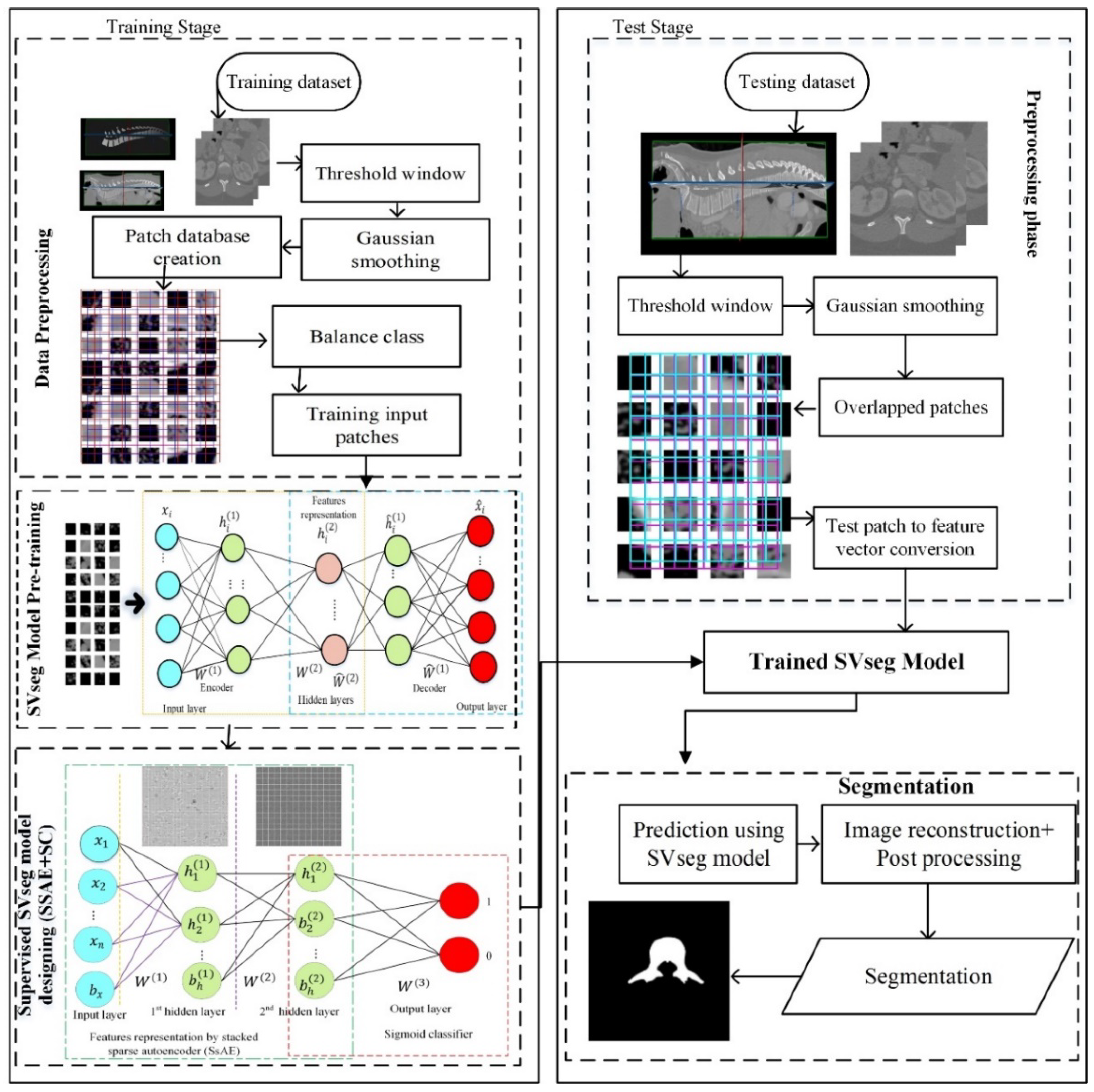
As shown in Figure 1, the proposed method is composed of four procedures: (i) data preprocessing; (ii) SVseg model pretraining; (iii) SSAE + SC for supervised SVseg model designing; and (iv) testing.
2.1. Data Preprocessing
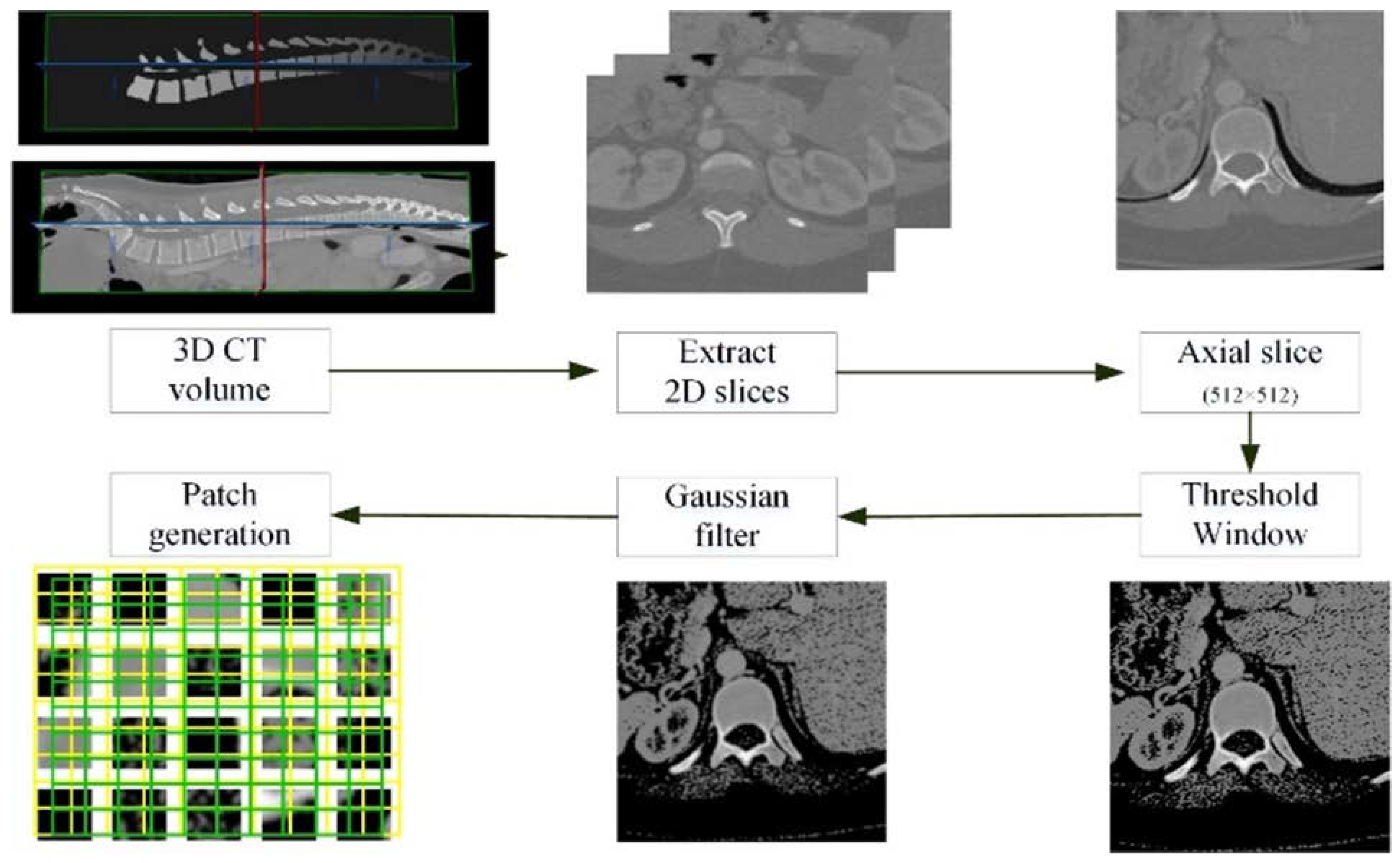
In the data preprocessing, the noise of the whole CT volume was filtered out by applying a rough threshold window. On the dataset, a slice-by-slice process was performed. The vertebrae have higher intensities in images than other tissues but are similar to different bone structures like ribs, so the algorithm learned the difference between vertebrae structures from other bony structures. A Gaussian filter with a sigma value of 1.5 was applied to control CT images’ smoothness as a preprocessing step for obtaining accurate segmentation and attenuating the effects of noisy pixels. The CT images of the spine were divided into 32 × 32 pixel overlapped patches. To create the overlapping patches, we used certain stride pixels. An image patch contains a total of 1024 pixels, and if these pixels are equal to or greater than 50%, then the patch is labeled 1 (vertebra patch); otherwise, it is labeled 0 (nonvertebra patch). There was an imbalance in the number of training patches between the two classes used for classification. Most training patches are labeled “0” because the vertebrae area in the images is smaller than the background area, which can lead to background bias. To solve this dilemma, it is necessary to strike a balance between the sizes of the positive and negative training image patches. We generated a balanced training set using a random undersampling function for negative samples (nonvertebrae patches). This improves the network’s accuracy and convergence rate during model training [50]. Figure 2 illustrates the data preprocessing.
2.2. SVseg Model Pretraining
In this work, we introduced a stacked sparse autoencoder [51] (SSAE) for high-level feature learning from overlapping image patches during training. An SSAE is an unsupervised technique of deep learning that contains basic layers for feature learning. In the following section, we first discuss the basic feature learning algorithm by sparse autoencoder and then introduce the stacking of sparse autoencoder; finally, we used a sigmoid classifier layer with unsupervised SSAE for fine-tuning the SVseg model.
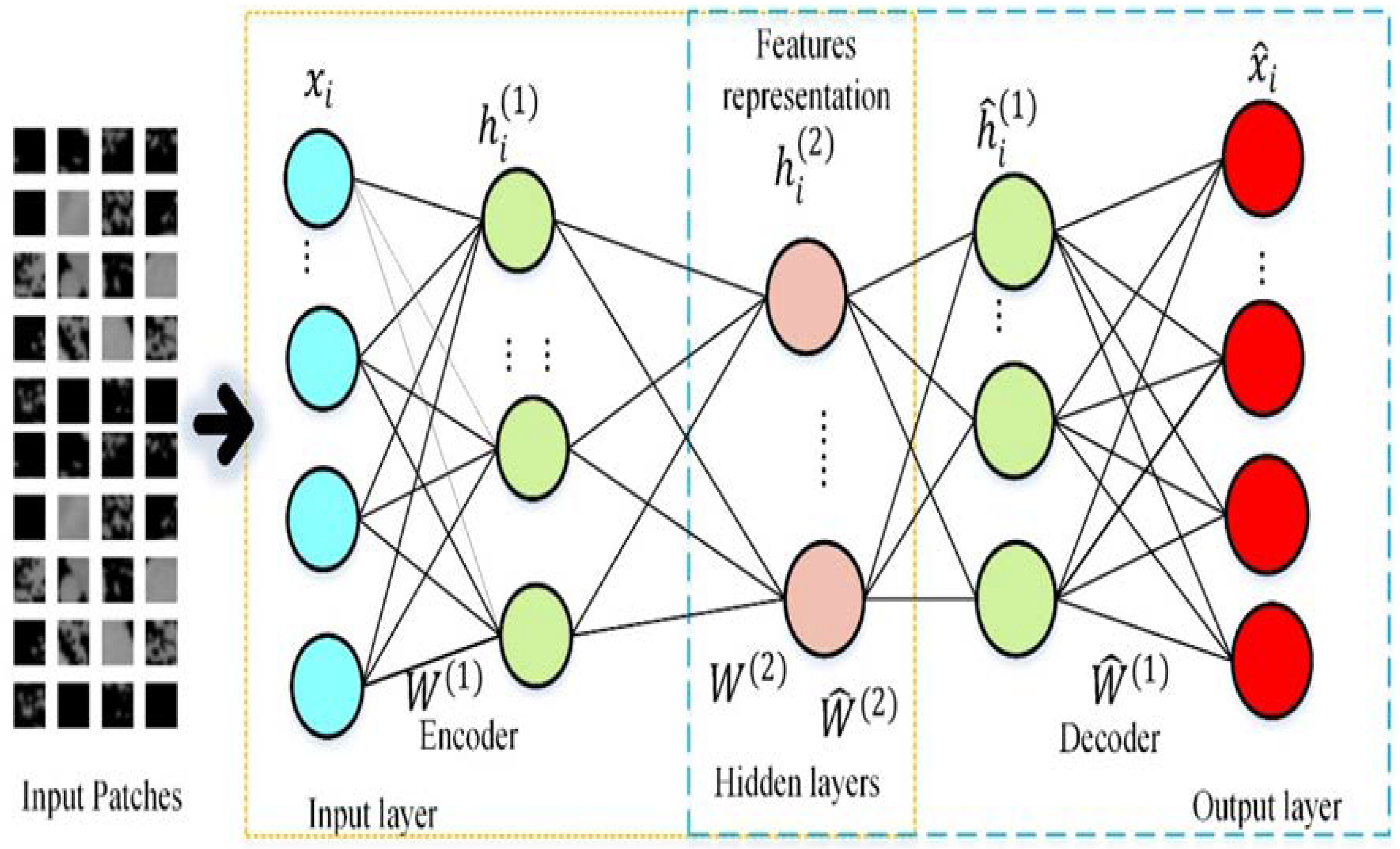
The fundamental unit for SSAE, autoencoder (AE) works for feedforward nonlinear neural network training. It is composed of three fundamental layers: an input, a hidden layer, and an output layer structure. There are a number of nodes that make up each layer of AE; these nodes establish full connections between the nodes of adjacent layers. Basically, the autoencoder consists of the encoder–decoder processing step, as shown in Figure 3. The input vector presentation is encoded in the encoding stage to link the input layer and the autoencoder’s hidden layer. In contrast, the autoencoder implies the input vector reconstruction from encoded features learning in the hidden layers in the decoding stage. The autoencoder’s purpose is to determine the input data representation that could be used to create the best reconstruction. A concatenated vector feature of an image patch was fed into AE in our method. Input image patches were given to AE in the training, and reducing the error factor for all network connection weights was performed as follows:
In Equation (1), are the weights, biases, and activation function of autoencoder parameters. Given an input vector , the autoencoder first encodes this input into the representation , where is the responses of hidden-layer neurons and h is the dimension that corresponds to the number of neurons in the hidden layer. The autoencoder decodes the original input from the encoding learning throughout the decoding process, . For effective feature extraction from input image patches, the autoencoder requires that the hidden layer dimension be less than the input layer’s dimensions; otherwise, error minimization would lead to a trivial solution. The authors of [52] determined that the feature learning of the autoencoder is similar to that of PCA.
Rather than a limitation of hidden layer dimension, an alternate approach called sparse autoencoder (SAE) imposed sparsity regularization on the autoencoder’s hidden layers. SAE implements the regularization of the hidden layer’s responses to avoid trivial solutions that the basic autoencoders tend towards. Those basic autoencoders required the hidden layer’s dimension to be less than the input layer’s dimension. Precisely, to make infinitesimal, the sparsity regularization is imposed on the autoencoder. To create a balance between the hidden layer’s sparsity and reconstruction power, for every input node, only the most suitable hidden nodes responses that drive the SAE to represent the training set in sparse features. It can be stated as follows:
where shows the balancing parameter between sparsity and reconstruction and the dimensions of the hidden layer are defined by M. The term , known as the Kullback–Leibler equation [53] (Equation (3)), shows the divergence in two Bernoulli distributions that have the probability . The sparsity is minimized when for each hidden neuron . From the image patches of vertebrae, the low-level features can be learned by SAE. However, due to variations in the appearance of vertebrae, low-level feature learning is insufficient. In contrast, abstract high-features are more robust to CT images’ inhomogeneity. Based on human perception, we applied SSAE for high-level feature learning based on low-level feature representation. The stacking of multiple SAEs, known as SSAE, contracts deep hierarchies. To learn abstract high-level features from input images patch, we stacked the SAE to feed the low-level SAE output layer as an input layer for the high-level SAE. This SSAE network uses an unsupervised method for pretraining the SVseg model. From input overlapping patches, the SSAE was trained without utilizing the label data.
2.3. SSAE + SC for Supervised SVseg Model Designing
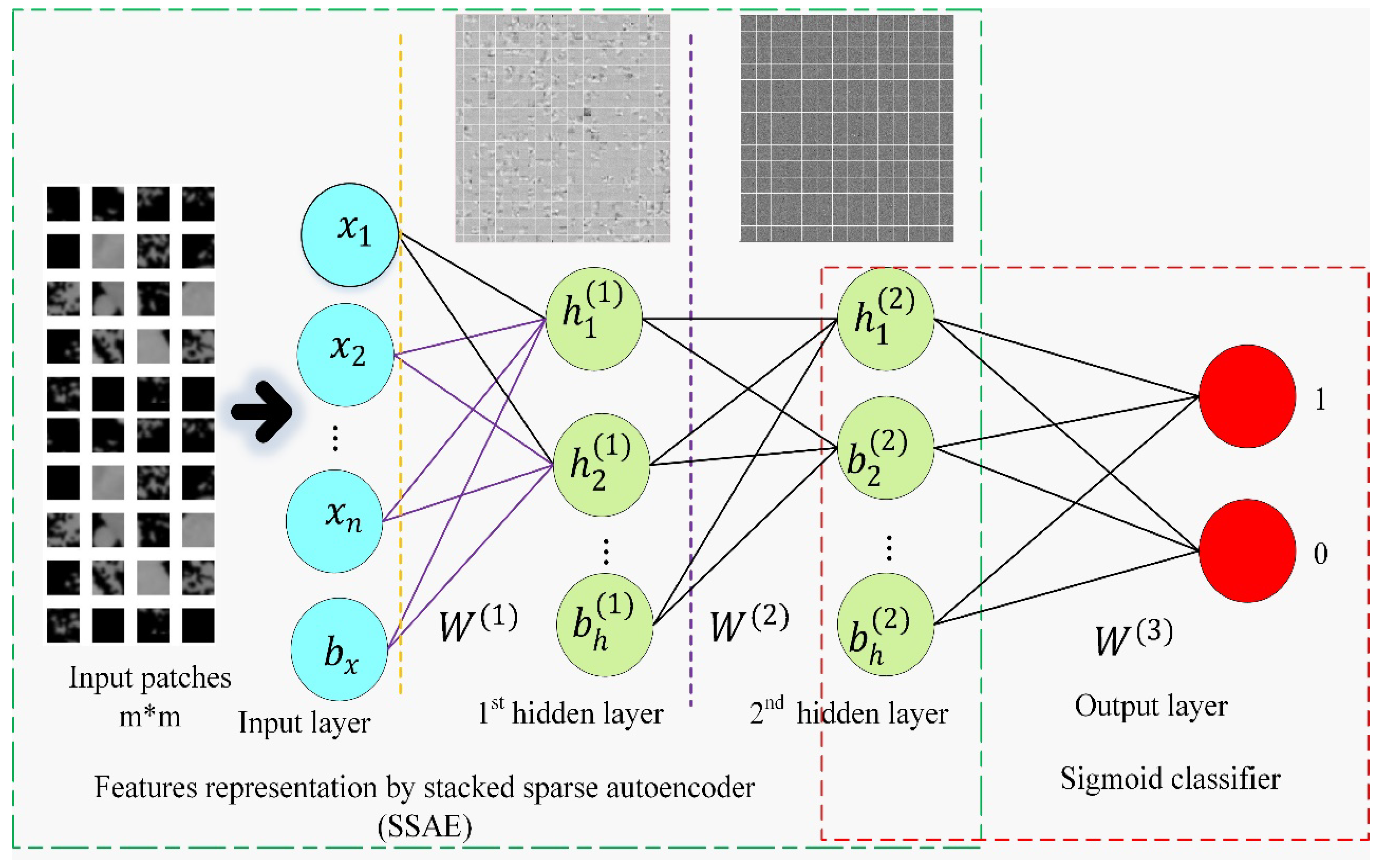
Since SSAE is trained in an unsupervised manner, the high-level feature representation is only data-adaptive, and not necessarily discriminative enough for separating the vertebra from background patches. To discriminate learned features [54,55], a supervised fine-tuned approach SSAE+SC (sigmoid classifier) [56] was used, as shown in Figure 4.
The proposed SVseg model contains four network layers: one input layer, two hidden layers, and one sigmoid layer. The training procedure consists of different stages. Firstly, a sparse autoencoder (SAE) was imposed on the overlapped patches in training data for primary feature learning by the adjustment of weight . After that, input pixels were given to this trained SAE for representation activations . The secondary presentation learning was obtained by using the primary representation as an input to the other SAE by the adjustment of the weight. These secondary representations were used for the sigmoid layer as input and to learn the mapping of to labels by the adjustment of the weight. Finally, one input and two hidden layers were stacked for making SSAE and a final sigmoid layer was added an output layer capable of detecting the vertebrae from the background. The SVseg model included the bottom-up training of SSAE in an unsupervised way, followed by a sigmoid classifier that used supervised learning for top layer training and fine-tuned the entire deep framework.
The number of nodes in the sigmoid layer was determined to be equal to the number of labels. The sigmoid layer in our method had two nodes, one for vertebra and the other for the background. The sigmoid layer predicts the likelihood of the label of the input data based on learned features, the second hidden layer representation . Other classifiers such as SVM and MLP can also be used. The SVM classifier calculates a posterior probability score for a pixel belonging to the target or background class. A probability image was created by reconstructing the score vector, which requires a high degree of generalization. On the other hand, a multilayer perceptron (MLP) is a feedforward neural network with a large number of layers and many nodes in each layer that cannot overcome the problem of overfitting and are stuck in local minima. However, sigmoid logistic regression allowed us to optimize the whole deep framework jointly through fine-tuning. The sigmoid classifier that generalizes logistic regression is shown in the below equation:
where x is the input and σ is the sigmoid output function [56] in Equation (4). For fine-tuning, the weights and biases of the sigmoid layer and SSAEs were optimized together, and the sigmoid layer was used for classification. The cost function can be minimized using a gradient descent-based model [51]. For every input , the two output values are calculated and these values are the classification probability of the input. This paper considers two class classification problems, and the label of the patch is {0, 1}, where 1 and 0 refer to vertebrae and nonvertebrae patches, respectively. It should be noted that the label information is not used in the SSAE learning procedure because SSAE learning is a method of unsupervised learning. After the high-level feature learning, the sigmoid layer (output layer) is fed the learned high-level representation of vertebrae structures along with its label (Figure 4). The trained model is then fed test patches, which return a 0 or 1 value indicating whether the input image patch represents a vertebra or not.
2.4. Testing
After training, the SVseg model is ready to test unseen vertebrae patches for model validation. Test image patches were fed to the SVseg model and produced a predicted value of one or zero, interpreted as the probability of corresponding to vertebra or background. Based on these results, a binary segmented image was obtained after reconstruction of the predicted patches. Due to the high contrast between vertebra, ribs, and other skeletal structural tissues, some background pixels were misclassified as vertebrae, while some vertebrae pixels were misclassified as background. Thus, these outliers were removed by applying morphological operations [57] such as dilation, erosion, and hole filling to improve the segmentation accuracy in postprocessing.
3. Experimental Setup
We intended to compare our proposed SVseg model with other segmentation algorithms. Our model’s performance was evaluated on the public dataset of segmentation challenge in MICCAI Computational Spine Imaging (CSI) 2014 [49].
3.1. Dataset
The datasets were collected at the Medical Center at the University of California, Irvine (Orange, CA, USA) [49]. The dataset contained a total of 15 CT images, 10 CT images (5595 slices) for the training, and five CT images (3418 slices) for the testing. Each CT scan covered the whole lumbar and thoracic spine and included complete vertebrae segmentation masks. The scanning settings were: slice thickness of 0.7–2.0 mm, voltage of 120 kVp, a kernel for soft tissue reconstruction, and intravenous contrast. The axial in-plane resolution varied between 0.3125 and 0.3613 .
3.2. Experiments
A given set of hyperparameters initialized the SSAE network. These parameters included framework parameters, weights of the sigmoid layer, number of layer’s hidden neurons, target activation for hidden neurons, sparsity penalty β, and L2 regularization λ. A random search [58] was used to find the optimal network structure in terms of performance. First, we tried to define the spectrum of hyperparameters, and then we selected the values randomly. We trained our framework with these selected values and repeated this process until we found the best productivity. For evaluation, the dataset was split into three subgroups , , and . From the 20 training CT images, we generated 651,712 overlapping image patches (325,856 vertebrae patches + 325,856 nonvertebrae patches). We randomly selected 80% of the patches for I_train and 20% for I_valid. The size of each slice was about 512 × 512 pixels. Training set I_train and I_valid contained 525,568 and 126,144 sample patches, respectively, which were used to train the SVseg model. The mini-batch size was set to 64 for efficient training, and I_train was divided into 8212 mini-batches and I_valid into 1971 mini-batches. The proposed method contained four network layers: one input layer with 1024 neurons; two hidden layers with 729 and 196 hidden neurons, respectively; and one sigmoid layer consisting of two neurons corresponding to the number of classes. Many experiments were conducted to determine the SVSeg model’s number of hidden layers and the number of nodes in each hidden layer. The performance of the models was monitored in each experiment until the SVseg model achieved its optimal performance (two hidden layers, the first with 729 nodes and the second with 196 nodes).
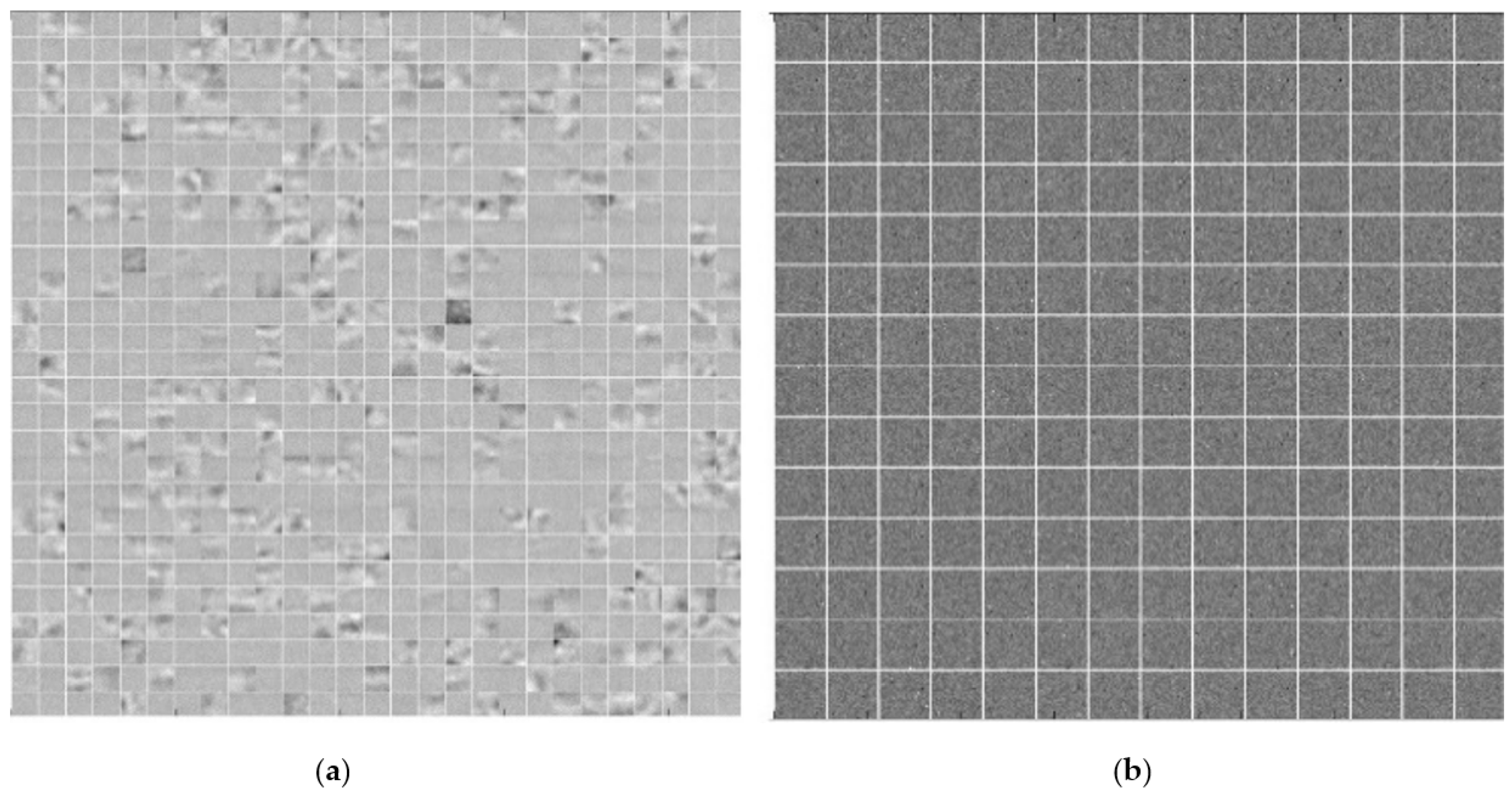
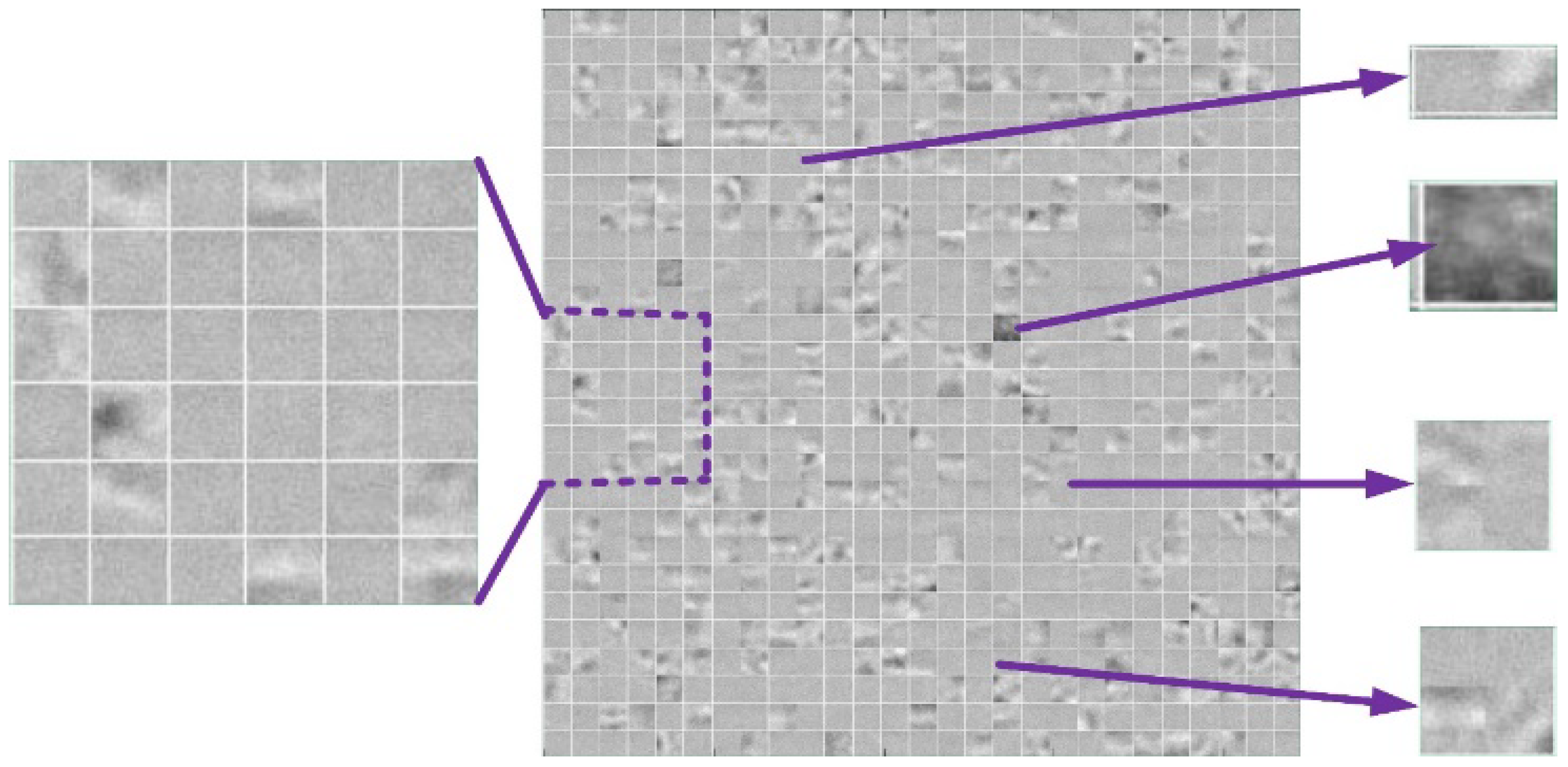
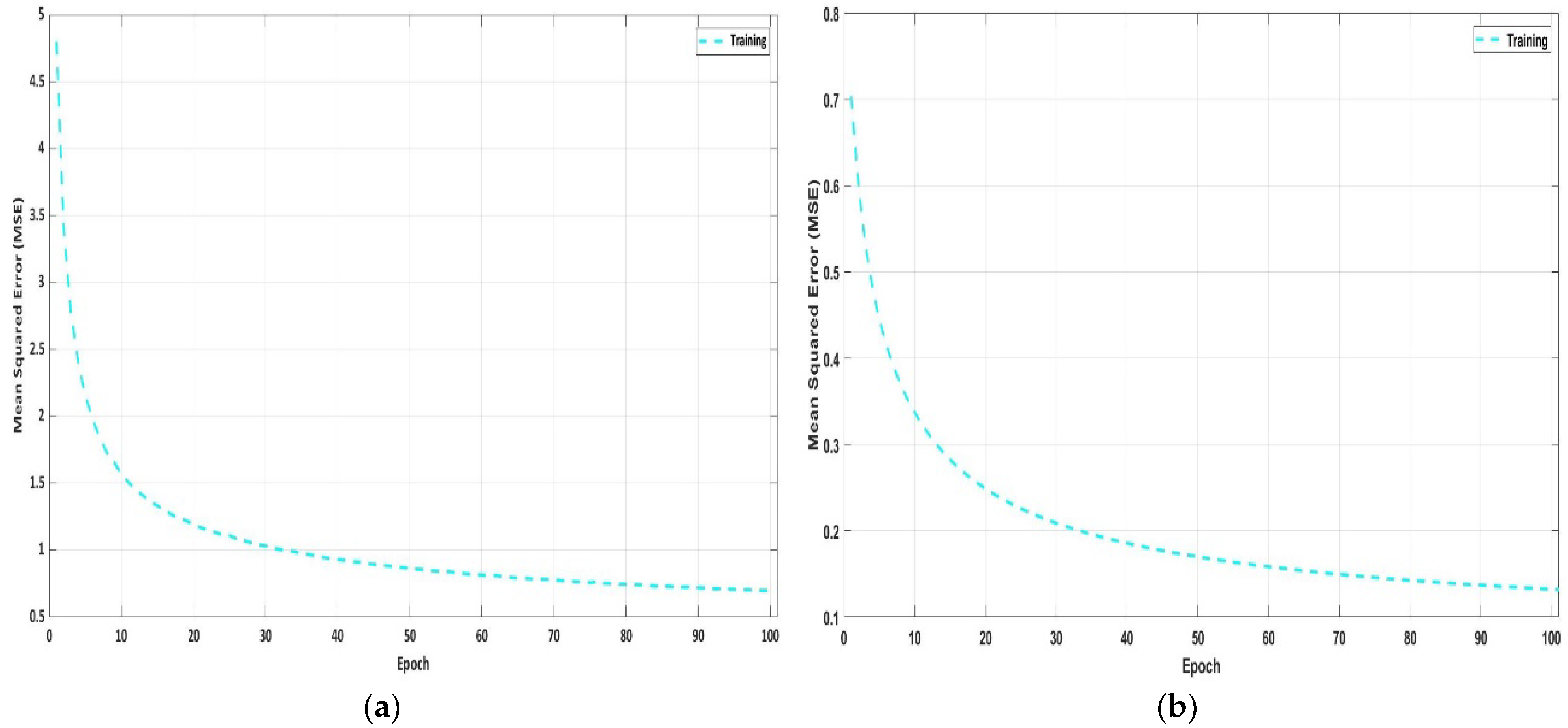
Figure 5 shows the visualization of the first and second hidden layers’ feature presentations by the four-layered SSAE based on the visualization model [59]. These features demonstrate that the model is capable of revealing vertebrae and nonvertebral structures from training patches. The learned feature representation in the first hidden layer (with 729 (27 × 27) nodes) indicates the vertebrae’s detailed boundary features and other structures as shown in Figure 5a, while feature representation in the second hidden layer (with 196 (14 × 14) nodes) expresses the high-level feature learning of vertebrae as shown in Figure 5b. The 6 × 6 zoomed image of the SSAE’s first hidden layer indicates weights at the left side, and the boundary and corner of vertebrae at the right side in Figure 6. Each square represents the weight between a single hidden node and the corresponding pixel in the original image. In the weight matrix, a gray pixel represents zero, whereas a white pixel represents a positive value. According to these findings, SVseg appears to be capable of learning useful high-level features that can be used to better describe vertebrae structures. The hyperparameters were selected to minimize the discrepancy between input and its reconstructions. In our work, this disparity was calculated as the mean square error (MSE). MSE is calculated between the input and reconstructed input from the AE decoder. Its gradually decreasing values relate to its saturation with respect to the number of epochs during the training phase.
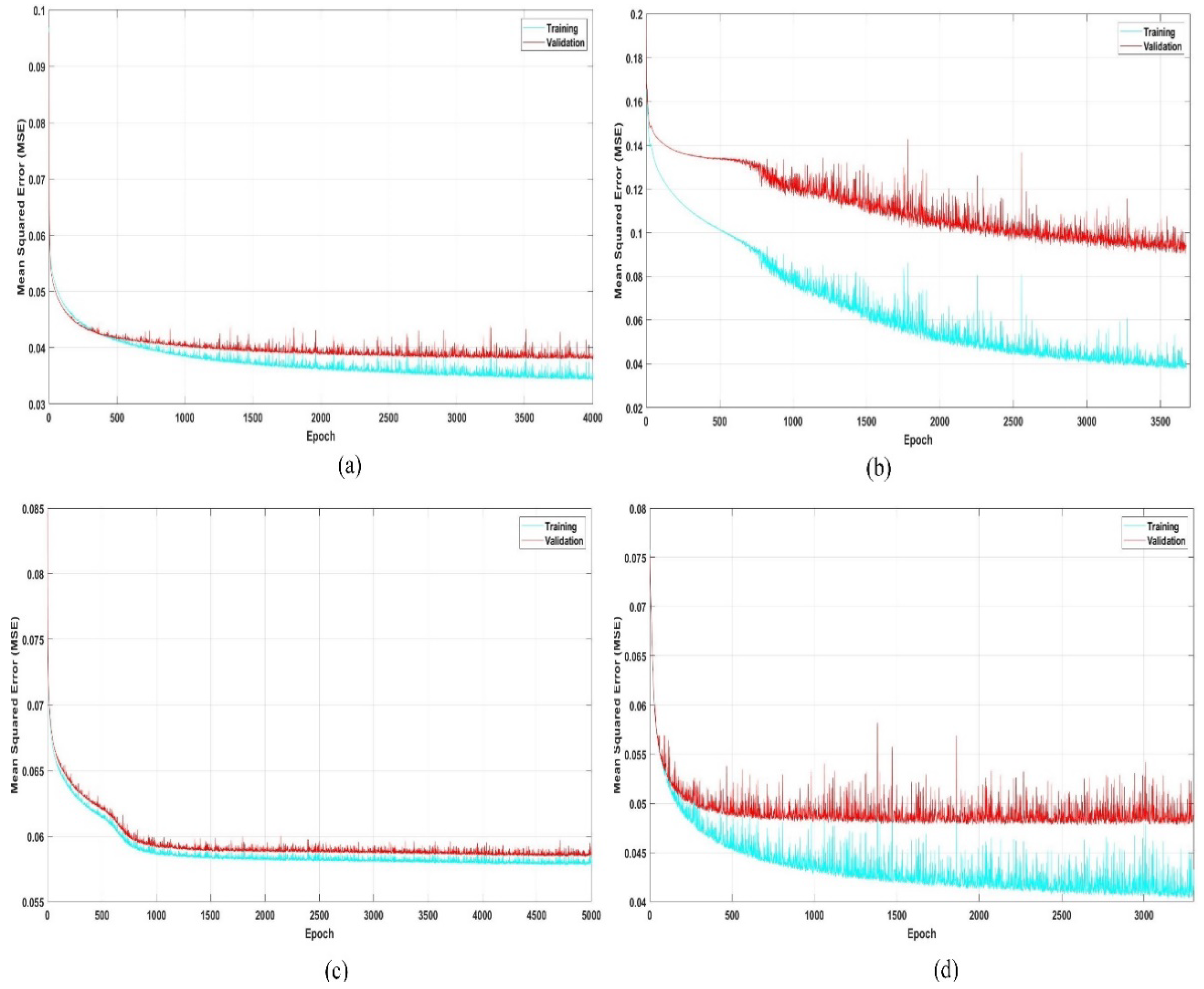
Figure 7 shows the SVseg model pretraining learning curve in an unsupervised fashion, where 100 epochs are used and no label data are provided. After the pretraining, the supervised SVseg model learning curve, MSE of training, and validation corresponding to a number of epochs are shown in Figure 8. Figure 8a shows the best fit curve for our model training with MSE of 0.034 for training and MSE of 0.038 for validation. The learning curve diverges rapidly before 700 epochs and then stabilizes after 2500 epochs. Figure 8b depicts the problem of overfitting caused by a deviation in the validation curve from the training curve. Figure 8c,d shows the poor training MSE graph with a low learning rate and small batch size, respectively. The heuristic approach was used to obtain the correct training curve, as illustrated in Figure 8a. Therefore, initialization of weight is important in deep learning.
3.3. Evaluation Metrics
In this study, the Dice similarity coefficient (DSC) [60], Jaccard similarity coefficient (JSC) [61], precision (PRE), and sensitivity (SEN) were used as quantitative assessment metrics to evaluate segmentation performance [20,29]. We evaluated true positives (TP), true negatives (TN), false positives (FP), and false negatives (FN) by comparing the true labels with predicted labels:
4. Results and Discussion
To demonstrate the efficiency of the SVseg model, the model was compared to five other state-of-the-art models. We, therefore, compared the SVseg to other models to evaluate the segmentation efficiency. The training procedures of AE + SC, StAE + SC, SAE + SC, 3SAE + SC, and 4SAE + SC were similar to the techniques used for SVseg, as shown in Figure 4.
(i) Autoencoder plus sigmoid classifier (AE + SC): The sparsity constraint on the hidden layer of AE as controlled by the parameter σ in Equation (2). If the sparsity constraint was removed by σ = 0 in Equation (2), the sparse AE was transformed into a single-layered AE. The input x of the sigmoid classifier in Equation (4) was learned via single-layer AE, and the SC was trained for model fine-tuning. Then, SC was used with AE to determine if a vertebra was present or absent inside each image patch.
(ii) Stacked Autoencoder plus sigmoid classifier (StAE + SC) is a neural network composed of many layers of basic AE with each layer’s outputs connected to the inputs of the subsequent layer. StAE is a two-layered fundamental AEs model. SC’s input x in Equation (4) is a feature learned from the pixel intensities of an image patch using a two-layer AEs.
(iii) Sparse autoencoder plus sigmoid classifier (SAE + SC): In this approach, the input x of SC in Equation (4) is a feature learned from the pixel intensities of an image patch using a single layer of Sparse AE.
(iv) Three-layer sparse autoencoder plus sigmoid classifier (3SAE + SC): This model is composed of three Sparse AE layers, with the outputs of each layer connected to the inputs of the subsequent layer. The first and second hidden layers have the same nodes as in our SVseg, and the third layer has 49 hidden nodes.
(v) Four-layer sparse autoencoder plus sigmoid classifier (4SAE + SC): This network is composed of four sparse AE layers and has the same parametric settings as the SVseg model but the third and fourth layers have 49 and 16 hidden nodes, respectively. An SC layer is attached at the end of network for fine-tuning. The 4SAE + SC model uses the same method for training as shown in Figure 4.
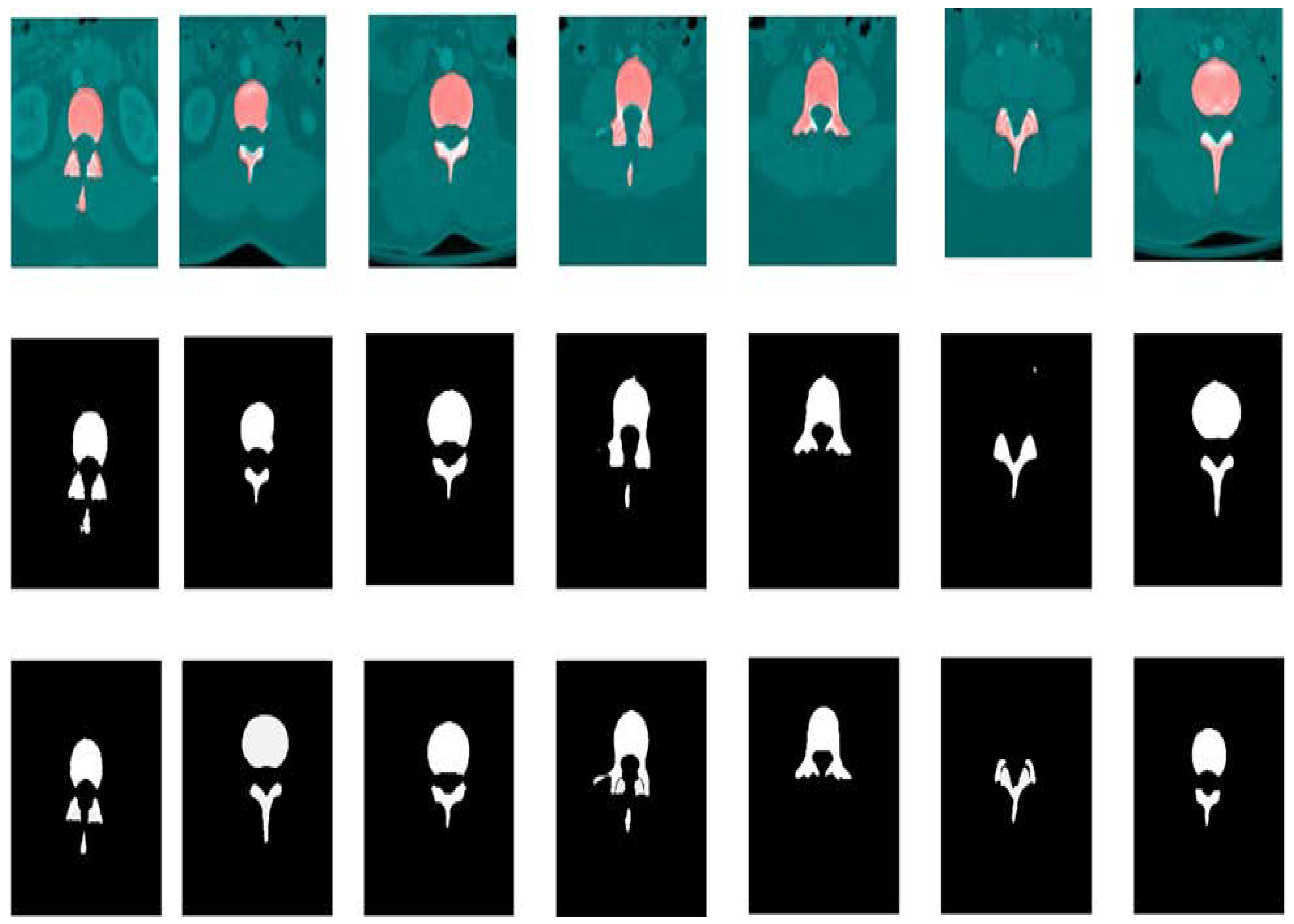
The quantitative performance of SVseg and different models was analyzed using the metrics in Equations (5)–(8), respectively. Table 1 indicates the means of DSC, JSC, PRE, and SEN of SVseg and comparative models. Table 1 shows that the SVseg model results give superior segmentation performance compared to the other models in all metrics. While the results tend to favor “deeper” architecture over “shallow” architecture in encoding high-level features from pixel intensities, the 3SAE + SC and 4SAE + SC models’ poor performance compared to the SVseg model suggests that adding more layers may cause an overfitting problem. Figure 9 shows the visualization of vertebrae segmentation results, randomly selected from five test cases based on our SVseg model.
4.1. Computational Cost
The experiments were carried out on a 1.80 GHz i7 CPU, 32 GB RAM, NVIDIA GeForce MX250 GPU using MATLAB 2018a environment. In this study, we compared SVseg’s computational efficiency to that of five other state-of-the-art approaches. Table 2 shows the execution times for each model. Regarding training time, the two autoencoder-based models that do not include sparsity required less training time than the three models with sparsity. In addition, as the number of layers in the architecture increased, more time was needed for training. In terms of run-time execution, our proposed SVseg model was more efficient than the other five models.
4.2. Discussion
As shown in Table 3, we also compared our SVseg model with classical segmentation algorithms including U-Net [62], DeepLabv3+ [63], MultiResUNet [64], Densely-UNet [65], and other well-known vertebrae segmentation methods. Table 3 indicates that the proposed SVseg model outperformed all the other models in terms of DSC and JSC. Compared with the classical U-Net [62], DeepLabv3+ [63], MultiResUNet [64], Densely-UNet [65], SpineParseNet [20], Mask R-CNN [66], and multiscale CNN [67] our SVseg model was significantly better by (3.79, 5.78), (13.86, 19.46), (1.90, 3.05), (4.23, 6.43), (0.07, 0.11), (18.19, 24.45), (0.89, 2.93) on average (DSC%, JSC%), respectively.
The SVseg model also achieved the best results compared with well-known vertebrae segmentation methods. For example, a mean 86.17% DICE score was reported for vertebrae segmentation using (D-TVNet) based on U-Net [68]. The experimental results showed that D-TVNet was unable to determine the critical points for measuring the spine curve angle using segmented bones. Additionally, when the noise was significant, and the bones not sharp, this method was ineffective at identifying them. While the D-TVNet method is capable of removing some noise from images, it can also accidentally remove relevant bones in some cases. In [29], a deep learning approach was proposed for automatic CT vertebra segmentation and achieved a 86.1% DICE score. The starting thoracic vertebrae have a lower DICE due to the influence of the ribs and intervertebral discs. This method segmented several bones not seen in the label annotations, resulting in misclassification and a low DICE score. These variables contributed to error segmentations. A deep learning patch-based technique for cervical vertebra segmentation in X-ray images was proposed in [32] with a DICE score of 84%, but this framework has a number of flaws. By eliminating outlier centers away from the vertebral curve, the center localization structure can be strengthened even further. The current framework for center localization was limited by the fact that it does not know which center belongs to which vertebra. In another paper [69], a DICE score of 87% was obtained using a deep learning approach on the thoracolumbar spine from CT images, but this approach omits information about a spine’s structural consistency. The result is odd behavior in which this method fails to segment parts of a vertebra, or, in some cases, entire vertebrae at the beginning or end of a spine. It should be investigated how such global systemic regularity can be imposed during the training phase. Table 3 shows that SVseg achieved the highest mean DSC and JSC for segmentation of vertebrae compared to all methods.
The above results and discussion prove that our proposed approach has the benefits of automatically learning high-level features from data images, rather than relying on handcrafted feature extraction, which often necessitates advanced engineering skills. SSAE differs from an autoencoder (AE) because it imposes sparsity on the mapped features, preventing the problem of trivial solutions when the dimensionality of hidden features exceeds the dimensions of input features. After stacking, SSAE can learn high-level features, similar to other deep learning techniques. Our SVseg model has the ability of high-level feature extraction by unsupervised learning, followed by training the sigmoid classifier in a supervised manner. The model was evaluated on a publicly CSI MICCAI dataset for training and testing.
As a result, the SVseg model achieved excellent segmentation of the vertebrae from CT images. To avoid potential issues caused by the limited amount of training data, we pretrained the model layer-by-layer, which allowed it to learn the hierarchy of features one layer at a time. Specifically, the previous layer’s learned features were fed into the next layer during each layer’s training. Secondly, the entire model was refined by only a few iterations during the fine-tuning stage, which is important for mitigating the overfitting problem. Thus, our model enhanced the accuracy and practicality of segmentation findings, enabling spine clinical diagnosis to be supported without relying on a complex network design.
We can also use transfer learning to avoid overfitting problems [47,70]. We can use other human organs’ CT images to initialize our model in the unsupervised pretraining process, obtaining a more general CT image appearance. We believe that, by performing this initialization, we will be able to improve the fine-tuning process and, as a result, overcome the small sample problem. In the fields of machine learning and computer vision, similar methods have been commonly used [47,70]. However, our model takes a long time to segment the vertebrae since it is implemented in MATLAB. Using Keras with a TensorFlow backend in Python is an option to improve the time efficiency of our approach. This will result in a decrease in computational time.
5. Conclusions
In conclusion, we proposed the SVseg model for CT image-based vertebrae segmentation. To overcome the difficulties of robust feature presentation caused by the large diversity of vertebra appearance, we proposed deep feature extraction by the SSAE architecture. The supervised sigmoid classifier fine-tunes the learned features from pretraining to estimate the target image’s vertebrae likelihood map. In this study, we found that the supervised fine-tuning step was positively impacted by sparsity regularization during training. The sparsity target forced the filters to collect more distinct features from image patches during the training phase. Our proposed method was tested on the publicly available CSI MICCAI dataset. When compared to other classical segmentation algorithms and well-known vertebrae segmentation methods, our model performed better in terms of segmentation accuracy. Finally, the SVseg model outperformed a variety of state-of-the-art methods in terms of vertebrae segmentation accuracy, both qualitatively and quantitatively. To better characterize vertebrae, we intend to extend our proposed model to other imaging modalities in the future and incorporate it with other deep learning feature extraction methods. Additionally, further validation, improvement, and implementation of our approach for additional applications like 3D medical image segmentation and multiclass classification will be our future focus.
Author Contributions
Conceptualization, S.F.Q. and L.S.; methodology, S.F.Q.; software, S.F.Q. and M.A.; validation, S.F.Q., L.S. and S.Q.; formal analysis, M.A., S.Q., S.S.Z. and M.A.A.; investigation, L.S.; resources, L.S.; data curation, S.F.Q.; writing—original draft preparation, S.F.Q. and L.S.; writing—review and editing, S.F.Q., L.S.; visualization, M.A., S.Q., S.S.Z. and M.A.A; supervision, L.S.; project administration, S.F.Q. and L.S.; funding acquisition, L.S. All authors have read and agreed to the published version of the manuscript.
Funding
This work was supported in part by the Natural Science Foundation of China through grant 91959108.
Institutional Review Board Statement
Not applicable.
Informed Consent Statement
Not applicable.
Data Availability Statement
The authors confirm that the data supporting the findings of this study are available within the article.
Conflicts of Interest
The authors declare no conflict of interest.
References
- Muñoz, H.E.; Yao, J.; Burns, J.E.; Summers, R.M. Detection of vertebral degenerative disc disease based on cortical shell unwrapping. In Proceedings of the International Conference on Medical Image Computing and Computer-Assisted Intervention, Novak, CL, USA, 29 March 2013; Aylward, S., Ed.; Volume 15, p. 86700C. [Google Scholar]
- Bourgeois, A.C.; Faulkner, A.R.; Pasciak, A.S.; Bradley, Y.C. The evolution of image-guided lumbosacral spine surgery. Ann. Transl. Med. 2015, 3, 69. [Google Scholar] [PubMed]
- Kim, G.-U.; Chang, M.C.; Kim, T.U.; Lee, G.W. Diagnostic modality in spine disease: A review. Asian Spine J. 2020, 14, 910. [Google Scholar] [CrossRef] [PubMed]
- Qadri, S.F.; Shen, L.; Ahmad, M.; Qadri, S.; Shamaila, S.; Khan, S. OP-convNet: A patch classification based framework for CT vertebrae segmentation. IEEE Access 2021, 9, 158227–158240. [Google Scholar] [CrossRef]
- Lim, P.H.; Bagci, U.; Bai, L. Introducing willmore flow into level set segmentation of spinal vertebrae. IEEE Trans. Biomed. Eng. 2013, 60, 115–122. [Google Scholar] [CrossRef]
- Huang, J.; Jian, F.; Wu, H.; Li, H. An improved level set method for vertebra CT image segmentation. Biomed. Eng. Online 2013, 12, 48. [Google Scholar] [CrossRef] [PubMed] [Green Version]
- Yao, J.; O’Connor, S.D.; Summers, R.M. Automated spinal column extraction and partitioning. In Proceedings of the Biomedical Imaging: Nano to Macro, Arlington, VA, USA, 6–9 April 2006; pp. 390–393. [Google Scholar]
- Naegel, B. Using mathematical morphology for the anatomical labeling of vertebrae from 3D CT-scan images. Comput. Med. Imaging Graph. 2007, 31, 141–156. [Google Scholar] [CrossRef]
- Kim, Y.; Kim, D. A fully automatic vertebra segmentation method using 3D deformable fences. Comput. Med. Imaging Graph. 2009, 33, 343–352. [Google Scholar] [CrossRef]
- Mastmeyer, A.; Engelke, K.; Fuchs, C.; Kalender, W.A. A hierarchical 3D segmentation method and the definition of vertebral body coordinate systems for QCT of the lumbar spine. Med. Image Anal. 2006, 10, 560–577. [Google Scholar] [CrossRef]
- Burnett, S.S.C.; Starkschall, G.; Stevens, C.W.; Liao, Z. A deformable-model approach to semi-automatic segmentation of CT images demonstrated by application to the spinal canal. Med. Phys. 2004, 31, 251–263. [Google Scholar] [CrossRef]
- Klinder, T.; Ostermann, J.; Ehm, M.; Franz, A.; Kneser, R.; Lorenz, C. Automated model-based vertebra detection, identification, and segmentation in CT images. Med. Image Anal. 2009, 13, 471–482. [Google Scholar] [CrossRef]
- Ma, J.; Lu, L.; Zhan, Y.; Zhou, X.; Salganicoff, M.; Krishnan, A. Hierarchical segmentation and identification of thoracic vertebra using learning-based edge detection and coarse-to-fine deformable model. In Proceedings of the International Conference on Medical Image Computing and Computer-Assisted Intervention, Beijing, China, 20–24 September 2010; pp. 19–27. [Google Scholar]
- Rasoulian, A.; Rohling, R.; Abolmaesumi, P. Lumbar spine segmentation using a statistical multi-vertebrae anatomical shape+pose model. IEEE Trans. Med. Imaging 2013, 32, 1890–1900. [Google Scholar] [CrossRef] [PubMed]
- Kadoury, S.; Labelle, H.; Paragios, N. Automatic inference of articulated spine models in CT images using high-order Markov Random Fields. Med. Image Anal. 2011, 15, 426–437. [Google Scholar] [CrossRef] [PubMed]
- Ibragimov, B.; Likar, B.; Pernuš, F.; Vrtovec, T. Shape representation for efficient landmark-based segmentation in 3-D. IEEE Trans. Med. Imaging 2014, 33, 861–874. [Google Scholar] [CrossRef] [PubMed]
- Zhang, L.; Wang, H. A novel segmentation method for cervical vertebrae based on PointNet++ and converge segmentation. Comput. Methods Programs Biomed. 2021, 200, 105798. [Google Scholar] [CrossRef] [PubMed]
- Tufail, A.B.; Ma, Y.-K.; Kaabar, M.K.A.; Rehman, A.U.; Khan, R.; Cheikhrouhou, O. Classification of Initial Stages of Alzheimer’s Disease through Pet Neuroimaging Modality and Deep Learning: Quantifying the Impact of Image Filtering Approaches. Mathematics 2021, 9, 3101. [Google Scholar] [CrossRef]
- Hirra, I.; Ahmad, M.; Hussain, A.; Usman Ashraf, M.; Saeed, I.A.; Qadri, S.F.; Alghamdi, A.M.; Alfakeeh, A.S. Breast Cancer Classification from Histopathological Images using Patch-based Deep Learning Modeling. IEEE Access 2021, 9, 24273–24287. [Google Scholar] [CrossRef]
- Pang, S.; Pang, C.; Zhao, L.; Chen, Y.; Su, Z.; Zhou, Y.; Huang, M.; Yang, W.; Lu, H.; Feng, Q. SpineParseNet: Spine Parsing for Volumetric MR Image by a Two-Stage Segmentation Framework with Semantic Image Representation. IEEE Trans. Med. Imaging 2021, 40, 262–273. [Google Scholar] [CrossRef]
- Masuzawa, N.; Kitamura, Y.; Nakamura, K.; Iizuka, S.; Simo-Serra, E. Automatic Segmentation, Localization, and Identification of Vertebrae in 3D CT Images Using Cascaded Convolutional Neural Networks. In Proceedings of the Lecture Notes in Computer Science (Including Subseries Lecture Notes in Artificial Intelligence and Lecture Notes in Bioinformatics), Lima, Peru, 4–8 October 2020; Volume 12266 LNCS, pp. 681–690. [Google Scholar]
- Chen, Y.; Gao, Y.; Li, K.; Zhao, L.; Zhao, J. Vertebrae Identification and Localization Utilizing Fully Convolutional Networks and a Hidden Markov Model. IEEE Trans. Med. Imaging 2020, 39, 387–399. [Google Scholar] [CrossRef]
- Ahmad, M.; Ai, D.; Xie, G.; Qadri, S.F.; Song, H.; Huang, Y.; Wang, Y.; Yang, J. Deep Belief Network Modeling for Automatic Liver Segmentation. IEEE Access 2019, 7, 20585–20595. [Google Scholar] [CrossRef]
- Ahmad, M.; Ding, Y.; Qadri, S.F.; Yang, J. Convolutional-neural-network-based feature extraction for liver segmentation from CT images. In Proceedings of the Eleventh International Conference on Digital Image Processing (ICDIP 2019), Guangzhou, China, 10–13 May 2019; Jiang, X., Hwang, J.-N., Eds.; Volume 1117934, p. 159. [Google Scholar]
- Sekuboyina, A.; Valentinitsch, A.; Kirschke, J.S.; Menze, B.H. A Localisation-Segmentation Approach for Multi-label Annotation of Lumbar Vertebrae using Deep Nets. arXiv 2017, arXiv:1703.04347. [Google Scholar]
- Korez, R.; Likar, B.; Pernuš, F.; Vrtovec, T. Model-based segmentation of vertebral bodies from MR images with 3D CNNs. In Proceedings of the International Conference on Medical Image Computing and Computer-Assisted Intervention, Athens, Greece, 17–21 October 2016; pp. 433–441. [Google Scholar]
- Yang, D.; Xiong, T.; Xu, D.; Huang, Q.; Liu, D.; Zhou, S.K.; Xu, Z.; Park, J.; Chen, M.; Tran, T.D.; et al. Automatic vertebra labeling in large-scale 3D CT using deep image-to-image network with message passing and sparsity regularization. In Proceedings of the International Conference on Information Processing in Medical Imaging, Boone, NC, USA, 25–30 June 2017; pp. 633–644. [Google Scholar]
- Chen, H.; Shen, C.; Qin, J.; Ni, D.; Shi, L.; Cheng, J.C.Y.; Heng, P.-A. Automatic localization and identification of vertebrae in spine CT via a joint learning model with deep neural networks. In Proceedings of the International Conference on Medical Image Computing and Computer-Assisted Intervention, Munich, Germany, 5–9 October 2015; pp. 515–522. [Google Scholar]
- Qadri, S.F.; Ai, D.; Hu, G.; Ahmad, M.; Huang, Y.; Wang, Y.; Yang, J. Automatic Deep Feature Learning via Patch-Based Deep Belief Network for Vertebrae Segmentation in CT Images. Appl. Sci. 2019, 9, 69. [Google Scholar] [CrossRef] [Green Version]
- Qadri, S.F.; Ahmad, M.; Ai, D.; Yang, J.; Wang, Y. Deep Belief Network Based Vertebra Segmentation for CT Images. In Proceedings of the Chinese Conference on Image and Graphics Technologies; Wang, Y., Wang, S., Liu, Y., Yang, J., Yuan, X., He, R., Duh, H.B.-L., Eds.; Springer: Singapore, 2018; Volume 757, pp. 536–545. [Google Scholar]
- Liu, X.; Yang, J.; Song, S.; Cong, W.; Jiao, P.; Song, H.; Ai, D.; Jiang, Y.; Wang, Y. Sparse intervertebral fence composition for 3D cervical vertebra segmentation. Phys. Med. Biol. 2018, 63, 115010. [Google Scholar] [CrossRef] [PubMed]
- Al Arif, S.M.M.R.; Knapp, K.; Slabaugh, G. Fully automatic cervical vertebrae segmentation framework for X-ray images. Comput. Methods Programs Biomed. 2018, 157, 95–111. [Google Scholar] [CrossRef] [PubMed] [Green Version]
- Liao, H.; Mesfin, A.; Luo, J. Joint vertebrae identification and localization in spinal CT images by combining short- and long-range contextual information. IEEE Trans. Med. Imaging 2018, 37, 1266–1275. [Google Scholar] [CrossRef] [Green Version]
- Türk, F.; Lüy, M.; Baricsçi, N. Kidney and Renal Tumor Segmentation Using a Hybrid V-Net-Based Model. Mathematics 2020, 8, 1772. [Google Scholar] [CrossRef]
- Abraham, B.; Nair, M.S. Computer-aided classification of prostate cancer grade groups from MRI images using texture features and stacked sparse autoencoder. Comput. Med. Imaging Graph. 2018, 69, 60–68. [Google Scholar] [CrossRef]
- Li, G.; Han, D.; Wang, C.; Hu, W.; Calhoun, V.D.; Wang, Y.P. Application of deep canonically correlated sparse autoencoder for the classification of schizophrenia. Comput. Methods Programs Biomed. 2020, 183, 105073. [Google Scholar] [CrossRef]
- Hou, L.; Nguyen, V.; Kanevsky, A.B.; Samaras, D.; Kurc, T.M.; Zhao, T.; Gupta, R.R.; Gao, Y.; Chen, W.; Foran, D.; et al. Sparse autoencoder for unsupervised nucleus detection and representation in histopathology images. Pattern Recognit. 2019, 86, 188–200. [Google Scholar] [CrossRef]
- Li, S.; Jiang, H.; Bai, J.; Liu, Y.; Yao, Y.-D. Stacked sparse autoencoder and case-based postprocessing method for nucleus detection. Neurocomputing 2019, 359, 494–508. [Google Scholar] [CrossRef]
- Jia, W.; Muhammad, K.; Wang, S.H.; Zhang, Y.D. Five-category classification of pathological brain images based on deep stacked sparse autoencoder. Multimed. Tools Appl. 2019, 78, 4045–4064. [Google Scholar] [CrossRef]
- Qadri, S.F.; Zhao, Z.; Ai, D.; Ahmad, M.; Wang, Y. Vertebrae segmentation via stacked sparse autoencoder from computed tomography images. In Proceedings of the Eleventh International Conference on Digital Image Processing (ICDIP 2019), Guangzhou, China, 10–13 May 2019; Jiang, X., Hwang, J.-N., Eds.; p. 160. [Google Scholar]
- Adem, K.; Kiliçarslan, S.; Cömert, O. Classification and diagnosis of cervical cancer with softmax classification with stacked autoencoder. Expert Syst. Appl. 2019, 115, 557–564. [Google Scholar] [CrossRef]
- Ahmad, M.; Yang, J.; Ai, D.; Qadri, S.F.; Wang, Y. Deep-Stacked Auto Encoder for Liver Segmentation. In Proceedings of the Chinese Conference on Image and Graphics Technologies, Beijing, China, 30 June–1 July 2018; pp. 243–251. [Google Scholar]
- Xu, J.; Xiang, L.; Hang, R.; Wu, J. Stacked Sparse Autoencoder (SSAE) based framework for nuclei patch classification on breast cancer histopathology. IEEE Trans. Med. Imaging 2016, 35, 119–130. [Google Scholar] [CrossRef] [PubMed] [Green Version]
- Guo, Y.; Gao, Y.; Shen, D. Deformable MR Prostate Segmentation via Deep Feature Learning and Sparse Patch Matching. IEEE Trans. Med. Imaging 2016, 35, 1077–1089. [Google Scholar] [CrossRef] [PubMed] [Green Version]
- Hassan, T.M.; Elmogy, M.; Sallam, E.-S. Diagnosis of Focal Liver Diseases Based on Deep Learning Technique for Ultrasound Images. Arab. J. Sci. Eng. 2017, 42, 3127–3140. [Google Scholar] [CrossRef]
- Qadri, S.F.; Awan, S.A.; Amjad, M.; Anwar, M.; Shehzad, S. Applications, challenges, security of wireless body area networks (WBANs) and functionality of IEEE 802.15.4/zigbee. Sci. Int. 2013, 25, 697–702. [Google Scholar]
- Pan, S.J.; Yang, Q. A survey on transfer learning. IEEE Trans. Knowl. Data Eng. 2009, 22, 1345–1359. [Google Scholar] [CrossRef]
- Deng, J.; Dong, W.; Socher, R.; Li, L.-J.; Li, K.; Fei-Fei, L. Imagenet: A large-scale hierarchical image database. In Proceedings of the 2009 IEEE Conference on Computer Vision and Pattern Recognition, Miami, FL, USA, 20–25 June 2009; pp. 248–255. [Google Scholar]
- Yao, J.; Burns, J.E.; Forsberg, D.; Seitel, A.; Rasoulian, A.; Abolmaesumi, P.; Hammernik, K.; Urschler, M.; Ibragimov, B.; Korez, R.; et al. A multi-center milestone study of clinical vertebral CT segmentation. Comput. Med. Imaging Graph. 2016, 49, 16–28. [Google Scholar] [CrossRef] [Green Version]
- Shin, H.-C.; Roth, H.R.; Gao, M.; Lu, L.; Xu, Z.; Nogues, I.; Yao, J.; Mollura, D.; Summers, R.M. Deep convolutional neural networks for computer-aided detection: CNN architectures, dataset characteristics and transfer learning. IEEE Trans. Med. Imaging 2016, 35, 1285–1298. [Google Scholar] [CrossRef] [Green Version]
- Ng, A. Sparse Autoencoder; CS294A Lecture Notes; Stanford Univ.: Stanford, CA, USA, 2011; Available online: https://web.stanford.edu/class/cs294a/sparseAutoencoder_2011new.pdf (accessed on 28 January 2022).
- Bengio, Y. Deep learning of representations for unsupervised and transfer learning. In Proceedings of the ICML Workshop on Unsupervised and Transfer Learning, Bellevue, WA, USA, 2 July 2012; pp. 17–36. [Google Scholar]
- Kullback, S.; Leibler, R.A. On information and sufficiency. Ann. Math. Stat. 1951, 22, 79–86. [Google Scholar] [CrossRef]
- Rota Bulo, S.; Kontschieder, P. Neural decision forests for semantic image labelling. In Proceedings of the IEEE Conference on Computer Vision and Pattern Recognition, Columbus, OH, USA, 23–28 June 2014; pp. 81–88. [Google Scholar]
- Suk, H.-I.; Shen, D. Deep learning-based feature representation for AD/MCI classification. In Proceedings of the International Conference on Medical Image Computing and Computer-Assisted Intervention, Berlin/Heidelberg, Germany, 22 September 2013; pp. 583–590. [Google Scholar]
- Han, J.; Moraga, C. The influence of the sigmoid function parameters on the speed of backpropagation learning. In Proceedings of the International Workshop on Artificial Neural Networks, Berlin/Heidelberg, Germany, 7 June 1995; pp. 195–201. [Google Scholar]
- Kang, Y.; Engelke, K.; Kalender, W.A. A new accurate and precise 3-D segmentation method for skeletal structures in volumetric CT data. IEEE Trans. Med. Imaging 2003, 22, 586–598. [Google Scholar] [CrossRef]
- Bergstra, J.; Bengio, Y. Random search for hyper-parameter optimization. J. Mach. Learn. Res. 2012, 13, 281–305. [Google Scholar]
- Lee, H.; Grosse, R.; Ranganath, R.; Ng, A.Y. Convolutional deep belief networks for scalable unsupervised learning of hierarchical representations. In Proceedings of the 26th Annual International Conference on Machine Learning, Montreal, QC, Canada, 14–18 June 2009; pp. 609–616. [Google Scholar]
- Dice, L.R. Measures of the amount of ecologic association between species. Ecology 1945, 26, 297–302. [Google Scholar] [CrossRef]
- Jaccard, P. Étude comparative de la distribution florale dans une portion des Alpes et des Jura. Bull. Soc. Vaud. Sci. Nat. 1901, 37, 547–579. [Google Scholar]
- Ronneberger, O.; Fischer, P.; Brox, T. U-net: Convolutional networks for biomedical image segmentation. In Proceedings of the International Conference on Medical Image Computing and Computer-Assisted Intervention, Munich, Germany, 5–9 October 2015; pp. 234–241. [Google Scholar]
- Chen, L.-C.; Zhu, Y.; Papandreou, G.; Schroff, F.; Adam, H. Encoder-decoder with atrous separable convolution for semantic image segmentation. In Proceedings of the European Conference on Computer Vision (ECCV), Munich, Germany, 8–14 September 2018; pp. 801–818. [Google Scholar]
- Wang, Z.; Zhang, Z.; Voiculescu, I. RAR-U-NET: A Residual Encoder to Attention Decoder by Residual Connections Framework for Spine Segmentation Under Noisy Labels. In Proceedings of the 2021 IEEE International Conference on Image Processing (ICIP), Anchorage, AK, USA, 19–22 September 2021; pp. 21–25. [Google Scholar]
- Kolařík, M.; Burget, R.; Uher, V.; Říha, K.; Dutta, M. Optimized High Resolution 3D Dense-U-Net Network for Brain and Spine Segmentation. Appl. Sci. 2019, 9, 404. [Google Scholar] [CrossRef] [Green Version]
- Wang, R.; Yi Voon, J.H.; Ma, D.; Dabiri, S.; Popuri, K.; Beg, M.F. Vertebra Segmentation for Clinical CT Images Using Mask R-CNN. In 8th European Medical and Biological Engineering Conference, Proceedings of the EMBEC 2020, Portorož, Slovenia, 29 November–3 December 2021; Springer: Cham, Switzerland, 2021; Volume 80, pp. 1156–1165. ISBN 9783030646097. [Google Scholar]
- Whitehead, W.; Moran, S.; Gaonkar, B.; Macyszyn, L.; Iyer, S. A deep learning approach to spine segmentation using a feed-forward chain of pixel-wise convolutional networks. In Proceedings of the 2018 IEEE 15th International Symposium on Biomedical Imaging (ISBI 2018), Washington, DC, USA, 4–7 April 2018; Volume 2018, pp. 868–871. [Google Scholar]
- Lyu, J.; Bi, X.; Banerjee, S.; Huang, Z.; Leung, F.H.F.; Lee, T.T.-Y.; Yang, D.-D.; Zheng, Y.-P.; Ling, S.H. Dual-task ultrasound spine transverse vertebrae segmentation network with contour regularization. Comput. Med. Imaging Graph. 2021, 89, 101896. [Google Scholar] [CrossRef] [PubMed]
- Sekuboyina, A.; Kukačka, J.; Kirschke, J.S.; Menze, B.H.; Valentinitsch, A. Attention-driven deep learning for pathological spine segmentation. In Proceedings of the International Workshop and Challenge on Computational Methods and Clinical Applications in Musculoskeletal Imaging, Quebec City, QC, Canada, 10 September 2017; pp. 108–119. [Google Scholar]
- Van Opbroek, A.; Ikram, M.A.; Vernooij, M.W.; De Bruijne, M. Transfer learning improves supervised image segmentation across imaging protocols. IEEE Trans. Med. Imaging 2015, 34, 1018–1030. [Google Scholar] [CrossRef] [Green Version]
Figure 1.
The flowchart of the proposed SVseg model (training stage and testing stage): SVseg consists of four steps: (i) data preprocessing; (ii) SVseg model pretraining; (iii) SSAE + SC for supervised SVseg model designing; and (iv) testing.
Figure 1.
The flowchart of the proposed SVseg model (training stage and testing stage): SVseg consists of four steps: (i) data preprocessing; (ii) SVseg model pretraining; (iii) SSAE + SC for supervised SVseg model designing; and (iv) testing.

Figure 2.
Examples of data preprocessing: 2D axial (512 × 512 pixels) slices are extracted from the 3D CT volume, a threshold window is applied, and a Gaussian smoothing filter is used on these slices; then images are divided into 32 × 32-pixel square patches (vertebrae and nonvertebrae patches).
Figure 2.
Examples of data preprocessing: 2D axial (512 × 512 pixels) slices are extracted from the 3D CT volume, a threshold window is applied, and a Gaussian smoothing filter is used on these slices; then images are divided into 32 × 32-pixel square patches (vertebrae and nonvertebrae patches).

Figure 3.
Architecture illustration of high-level feature learning of vertebral input image patches using an autoencoder with encoder and decoder networks.
Figure 3.
Architecture illustration of high-level feature learning of vertebral input image patches using an autoencoder with encoder and decoder networks.

Figure 4.
Illustration of unsupervised SSAE fine-tuned by adding a sigmoid classifier (output layer) for the supervised SVseg model design to classify the image patches into vertebrae or nonvertebrae.
Figure 4.
Illustration of unsupervised SSAE fine-tuned by adding a sigmoid classifier (output layer) for the supervised SVseg model design to classify the image patches into vertebrae or nonvertebrae.

Figure 5.
Visualization of high-level feature presentation extracted from input pixel intensities of our proposed two-hidden-layer SVseg model with sparsity constraint of 0.15 and sparsity regularization of 0.20. (a) The learned feature representation in the first hidden layer with 729 nodes. The learned high-level feature representation in the second hidden layer with 196 nodes is shown in (b). As anticipated, (a) illustrates detailed border features of vertebrae and other tissue, whereas (b) illustrates high-level vertebral features.

Figure 6.
The visualizations of SSAE’s first hidden layer expresses the learned feature representation (center image). The 6 × 6 zoomed image shows the weights of first hidden layer (left image), and four random weights from the 729-node hidden layer (right images).
Figure 6.
The visualizations of SSAE’s first hidden layer expresses the learned feature representation (center image). The 6 × 6 zoomed image shows the weights of first hidden layer (left image), and four random weights from the 729-node hidden layer (right images).

Figure 7.
Pretraining graph of SSAE for the unsupervised analysis of two hidden layers: (a) first hidden layer with 729 nodes; (b) second hidden layer with 196 nodes; 100 epochs are used.
Figure 7.
Pretraining graph of SSAE for the unsupervised analysis of two hidden layers: (a) first hidden layer with 729 nodes; (b) second hidden layer with 196 nodes; 100 epochs are used.

Figure 8.
Learning curves of SSAEs model during different experiments. (a) Best fit curve for our model training with MSE of 0.034 for training and MSE of 0.038 for validation; 4000 epochs were used and the mini-batch size was set to 64 for efficient model training. The learning curve diverged rapidly before 700 epochs and then stabilized after 2500 epochs; (b) depicts the problem of overfitting caused by a deviation in the validation curve from the training curve; (c,d) show poor training MSE graphs with a low learning rate and small batch size, respectively.

Figure 9.
Visualization of vertebrae segmentation results, randomly selected from five test cases of the thoracolumbar spine database (mid-axial slices). The first row shows the segmentation superimposed on the image, the second row shows segmented images, and the last row shows ground truths.
Figure 9.
Visualization of vertebrae segmentation results, randomly selected from five test cases of the thoracolumbar spine database (mid-axial slices). The first row shows the segmentation superimposed on the image, the second row shows segmented images, and the last row shows ground truths.


Table 1.
Performance evaluation metrics (DSC, JSC, PRE, and SEN) of SVseg with various models AE + SC, StAE + SC, SAE+SC, 3SAE + SC, and 4SAE for vertebrae segmentation on MACCAI CSI dataset.
Table 1.
Performance evaluation metrics (DSC, JSC, PRE, and SEN) of SVseg with various models AE + SC, StAE + SC, SAE+SC, 3SAE + SC, and 4SAE for vertebrae segmentation on MACCAI CSI dataset.
| Methods | DSC (%) | JSC (%) | PRE (%) | SEN (%) |
|---|---|---|---|---|
| AE + SC | 78.91 | 65.17 | 82.57 | 79.61 |
| StAE + SC | 83.39 | 71.51 | 88.17 | 85.71 |
| SAE + SC | 81.41 | 69.65 | 85.83 | 78.63 |
| 3SAE + SC | 85.12 | 74.09 | 90.59 | 88.41 |
| 4SAE + SC | 84.73 | 73.51 | 85.33 | 90.13 |
| SVseg (proposed) | 87.39 | 77.60 | 91.53 | 90.88 |
Table 2.
The execution time of AE + SC, StAE + SC, SAE + SC, 3SAE + SC, and 4SAE + SC trained on the training dataset and the time required to evaluate them on a test image of 512 × 512 pixels.
Table 2.
The execution time of AE + SC, StAE + SC, SAE + SC, 3SAE + SC, and 4SAE + SC trained on the training dataset and the time required to evaluate them on a test image of 512 × 512 pixels.
| Methods | Training Time (h) | Segmentation Time (s) |
|---|---|---|
| AE + SC | 21.05 | 16 |
| StAE + SC | 22.16 | 19 |
| SAE + SC | 23.07 | 13 |
| 3SAE + SC | 26.47 | 23 |
| 4SAE + SC | 37.22 | 23 |
| SVseg Model | 22.35 | 12 |
Table 3.
The SVseg model achieved the highest mean DSC (%) and JSC (%) compared with classical segmentation algorithms and also other vertebrae segmentation methods.
Table 3.
The SVseg model achieved the highest mean DSC (%) and JSC (%) compared with classical segmentation algorithms and also other vertebrae segmentation methods.
| Methods | Backbone | DSC (%) | (JSC) (%) |
|---|---|---|---|
| Classical U-Net [62] | U-Net | 83.60 | 71.82 |
| DeepLabv3+ [63] | DeepLabv3+ | 73.53 | 58.14 |
| MultiResUNet [64] | U-Net | 85.42 | 74.55 |
| Densely-UNet [65] | 3DU-Net | 83.16 | 71.17 |
| SpineParseNet [20] | 3D-GCSN, 2DResUNet | 87.32 | 77.49 |
| Mask R-CNN [66] | ResNet 101 | 69.20 | 53.15 |
| Multiscale CNN [67] | FCN | 86.50 | 74.67 |
| D-TVNet [68] | U-Net | 86.68 | 76.49 |
| PaDBN [29] | DBN | 86.10 | 75.59 |
| S. Al Arif et al. [32] | U-Net | 84.00 | 72.41 |
| A. Sekuboyina et al. [69] | U-Net | 87.00 | 76.99 |
| SVseg Model (proposed) | SSAE | 87.39 | 77.60 |
Publisher’s Note: MDPI stays neutral with regard to jurisdictional claims in published maps and institutional affiliations. |
© 2022 by the authors. Licensee MDPI, Basel, Switzerland. This article is an open access article distributed under the terms and conditions of the Creative Commons Attribution (CC BY) license (https://creativecommons.org/licenses/by/4.0/).
Share and Cite
MDPI and ACS Style
Qadri, S.F.; Shen, L.; Ahmad, M.; Qadri, S.; Zareen, S.S.; Akbar, M.A. SVseg: Stacked Sparse Autoencoder-Based Patch Classification Modeling for Vertebrae Segmentation. Mathematics 2022, 10, 796. https://doi.org/10.3390/math10050796
AMA Style
Qadri SF, Shen L, Ahmad M, Qadri S, Zareen SS, Akbar MA. SVseg: Stacked Sparse Autoencoder-Based Patch Classification Modeling for Vertebrae Segmentation. Mathematics. 2022; 10(5):796. https://doi.org/10.3390/math10050796
Chicago/Turabian StyleQadri, Syed Furqan, Linlin Shen, Mubashir Ahmad, Salman Qadri, Syeda Shamaila Zareen, and Muhammad Azeem Akbar. 2022. "SVseg: Stacked Sparse Autoencoder-Based Patch Classification Modeling for Vertebrae Segmentation" Mathematics 10, no. 5: 796. https://doi.org/10.3390/math10050796
Note that from the first issue of 2016, this journal uses article numbers instead of page numbers. See further details here.