
Novel Analysis of the Fractional-Order System of Non-Linear Partial Differential Equations with the Exponential-Decay Kernel


1
Department of Mathematics, College of Science, University of Bisha, P.O. Box 511, Bisha 61922, Saudi Arabia
2
Department of Mathematics, Faculty of Science, University of Ha’il, Ha’il 2440, Saudi Arabia
3
Department of Mathematics, Faculty of Science, Khon Kaen University, Khon Kaen 40002, Thailand
*
Author to whom correspondence should be addressed.
Mathematics 2022, 10(4), 615; https://doi.org/10.3390/math10040615
Submission received: 28 January 2022
/
Revised: 10 February 2022
/
Accepted: 14 February 2022
/
Published: 17 February 2022
(This article belongs to the Special Issue Computational, Experimental, and Theoretical Aspect of Fractional Order Operators)
Abstract
:This article presents a homotopy perturbation transform method and a variational iterative transform method for analyzing the fractional-order non-linear system of the unsteady flow of a polytropic gas. In this method, the Yang transform is combined with the homotopy perturbation transformation method and the variational iterative transformation method in the sense of Caputo–Fabrizio. A numerical simulation was carried out to verify that the suggested methodologies are accurate and reliable, and the results are revealed using graphs and tables. Comparing the analytical and actual solutions demonstrates that the proposed approaches are effective and efficient in investigating complicated non-linear models. Furthermore, the proposed methodologies control and manipulate the achieved numerical solutions in a very useful way, and this provides us with a simple process to adjust and control the convergence regions of the series solution.
1. Introduction
In the last few centuries, fractional derivative have been applied to solve several physical models, and these representations have been very good at modeling the real world. Numerous fundamental definitions of fractional derivatives were introduced by Atangana–Baleanu, Caputo–Fabrizio, Liouville–Caputo, Riemann–Liouville, Riesz, Weyl, Grunwald–Letnikov, and Hadamard, among others [1,2,3,4,5,6]. Numerous non-linear problems have been established and widely applied in applied sciences such as biology, mathematics, chemistry, and numerous classical mechanics fields such as fluid mechanics, condensed matter physics, transport phenomena, theoretical physics, and non-linear optics over the last few decades. When dealing with linear problems, it is hard to determine the actual conclusion of non-linear equations, which is vital for defining the features and attributes of physical events [7,8,9]. Several useful techniques have been used to investigate non-linear fractional partial differential equations (PDEs), for instance the variational iterative transformation technique [10], the natural Adomian decomposition technique [11,12,13,14], the homotopy perturbation transformation technique [15,16], the homotopy analysis transformation technique [17,18], the q-homotopy analysis transformation technique [19,20,21], the finite element technique [22,23], the finite difference technique [24], the reduced differential transformation technique [25,26,27], and so on.
Here, we stud a fractional gas dynamics system model that describes the evolution of the two-dimensional unsteady flow of a perfect gas. In astrophysics, the polytropic gas is defined as [28]:
in which represents the energy density, represents the total energy of the gas, represents the container volume, h represents a constant, and m represents the polytropic index. Two examples of such gases are degenerated electron gas and adiabatic gas. Polytropic gases are studied extensively in astrophysics and cosmology [29], and these gases can act similarly to dark energy [30]. Consider the following set of gas dynamic equations that describe the behavior of an unsteady flow of any ideal gas [31,32]:
under initial conditions:
where and are the velocity components, is the density, is the pressure, q is time, and is the ratio of the heat capacity, which denotes the adiabatic index.
In 1999, the homotopy perturbation method (HPM) was constructed by [33], which merges the homotopy method and the classic perturbation technique, which has been widely utilized in linear and non-linear problems [34,35,36]. The HPM is significant because it eliminates the necessity for a small parameter in the problems, therefore avoiding the difficulties associated with the standard perturbation methods. The primary aim of this study was to apply the HPM to the analysis of fractional-order non-linear gas dynamic equations by applying a newly presented integral transform called the “Yang transform” [37]. We gain a power-series-form result in the setting of a quick convergence series, where some termsare necessary to achieve very efficient solutions. There is no requirement for a linearization or discretization of non-linear problems, and only a few of these methods can produce a result that can be calculated fast.
J.H. He was the first to suggest the variational iteration method. The approach provides the results as a quickly converging consecutive approximation, which may yield a precise solution if one exists [38,39,40]. It was discovered that a few terms can be employed for numerical purposes for concrete problems where a precise answer is not possible. Afshan et al. proposed a new modification for the variational iteration technique in [41]. The primary impetus for this modification was the combination of the functional corrections of the variational iteration technique and the Laplace transform.
2. Preliminaries and Concepts
Definition 1.
Definition 2.
The fractional CF integral is expressed as [42]:
Definition 3.
For , we show the following solution of the Laplace transform of the CF derivative [42]:
Definition 4.
The Yang transform of is expressed as [37]:
3. Remarks
The Yang transform of several valuable terms is described as:
Lemma 1.
Let the Laplace transform of is , then [43].
Proof.
From Equation (5), we can obtain the Yang transform by putting as:
Since , this implies that:
Putting in (8), we obtain:
Thus, from Equation (7), we obtain:
Furthermore, from Equations (5) and (8), we obtain:
The links (10) and (11) represent the duality connection among the Laplace and Yang transforms. □
Lemma 2.
Let be a continuous function; then, the Yang transform of the CF derivatives of is defined by [43]:
Proof.
The fractional Laplace transform of CF is defined as:
Additionally, we have the relationship between the Yang and Laplace properties, namely . To achieve the required answer, we put for v in Equation (13), and we obtain:
As a result, the proof is complete. □
4. Road Map of the Suggested Method
The analysis of non-linear fractional PDEs via the HPTM: Consider the non-linear function and the linear fractional as [43]:
where the term defines the source function. Applying the Yang transform to Equation (15), we obtain:
Implementing the inverse Yang transform, we obtain:
Now, we use the homotopy perturbation technique:
We decompose the non-linear function as:
where shows He’s polynomials and is determined with the help of the formula:
Putting Equations (18) and (19) in Equation (17), we obtain:
By analyzing the coefficient of in (21), we derive the following terms:
The achieved result of Equation (15) can be defined as follows:
5. Error Analysis and Convergence
The following theorems are foundational to address the original models (15), the convergence, and the error analysis.
Theorem 1.
Let be the exact solution of (15), and let and , where H defines the Hilbert space. Then, the obtained solution will be convergent if , i.e., for any , such that
Proof.
We make a sequence of
To obtain the proper result, we must show that forms a “Cauchy sequence.” Consider the following:
For , we obtain:
Since and is bounded, take , and we obtain Thus, forms a “Cauchy sequence” in H. That is, the following sequence is a convergent sequences with the limits for . As a result, the proof is complete. □
Theorem 2.
Let be finite and show the obtained series result. Let such that ; therefore, the following analysis yields the maximum absolute error.
Proof.
Since is finite, this implies that .
Consider:
As a result, the proof is complete. □
6. The General Discussion of the VITM
In this portion, we describe the VITM solution for the fractional-order PDEs.
with the initial conditions being:
where is the fractional Caputo operator of ℘, , and , are linear and non-linear terms, respectively, and , are the source functions.
7. Applications
7.1. Example 1
Consider the fractional scheme of the non-linear gas equations:
with the initial conditions:
where c is the real constant.
7.2. Case 1
First, we solve this system with the help of the HPTM.
Now, applying the Yang transform of Equation (37), we obtain:
Taking the inverse Yang transform, we obtain:
Implementing the HPM in Equation (41), we can obtain:
where , , , and are He’s polynomials, which signify the non-linear terms. The first few terms of He’s polynomials are suggested as:
On both sides of the comparison coefficient of p, we have:
The suggested problem is a series form result defined as results in Figure 1, Figure 2 and Figure 3:
7.3. Case 2
The approximate result by the VITM:
8. Results and Discussion
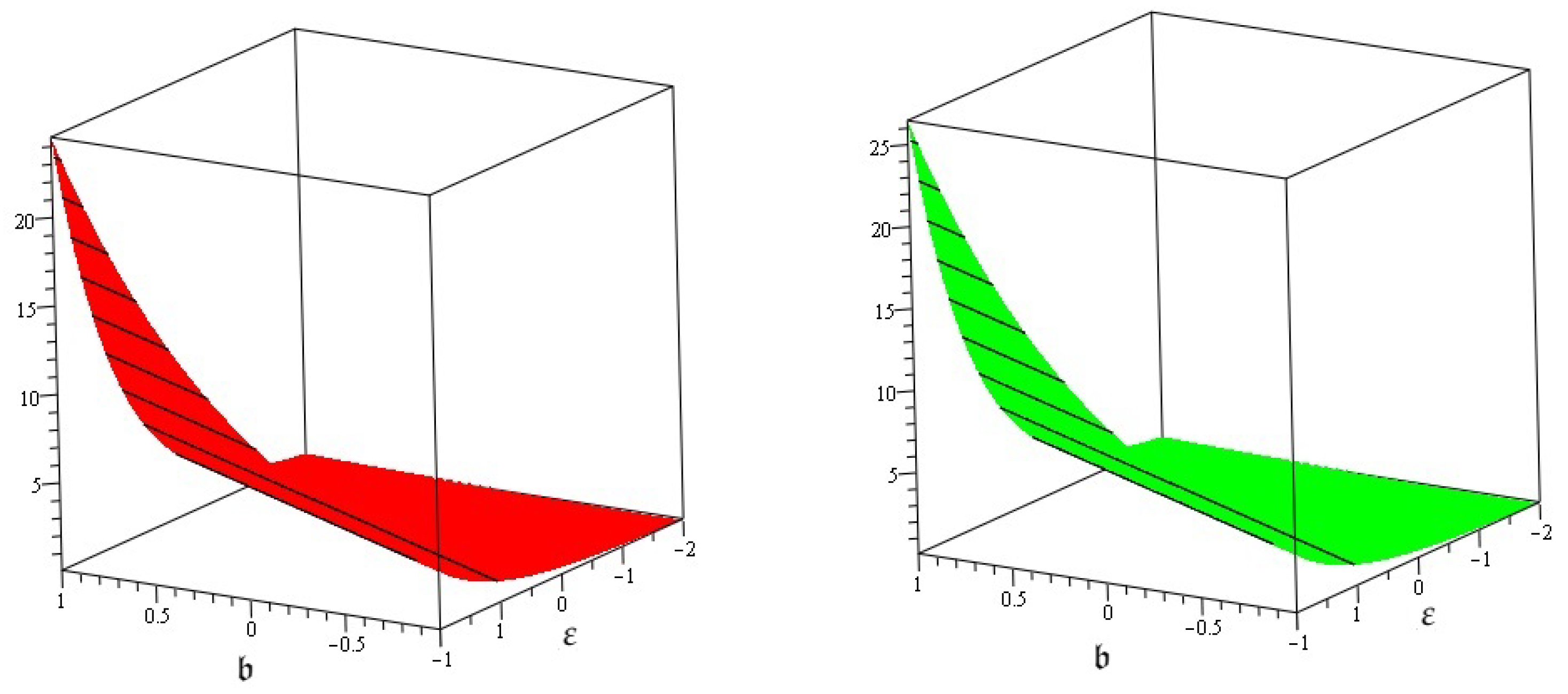
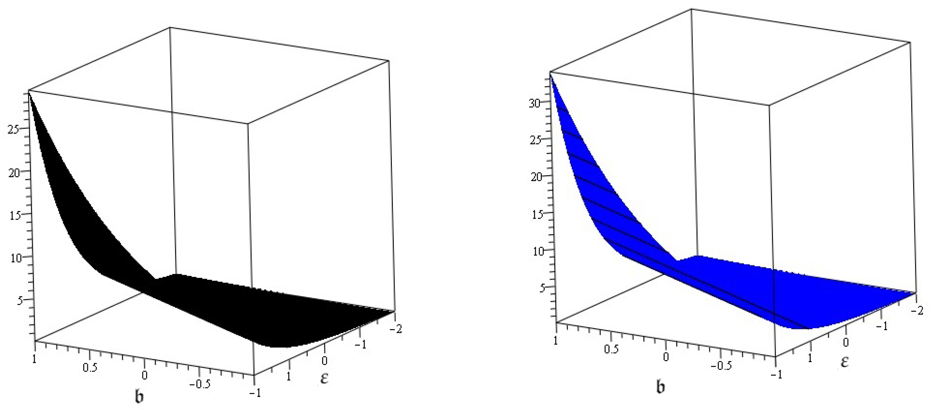
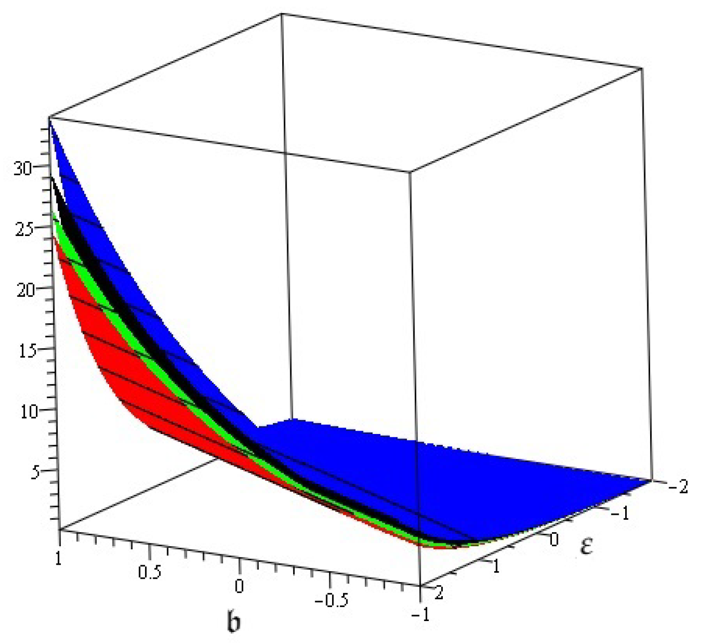
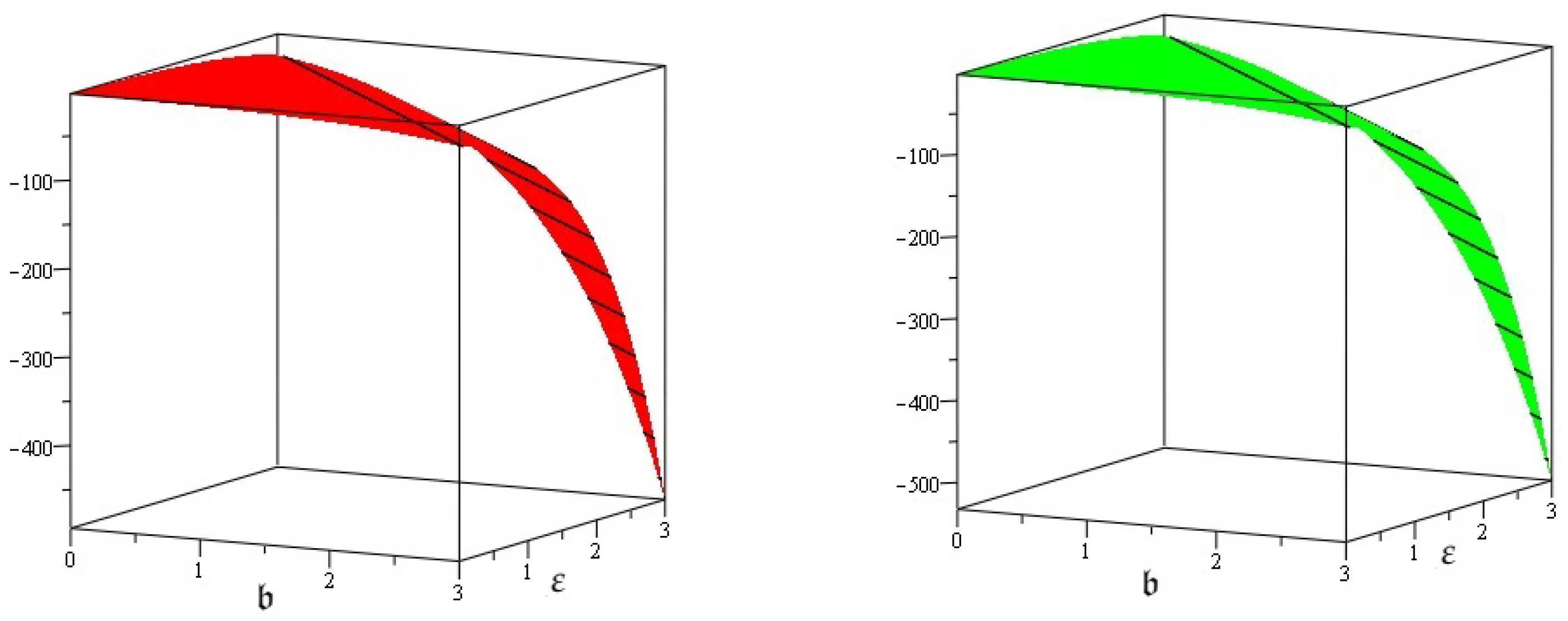
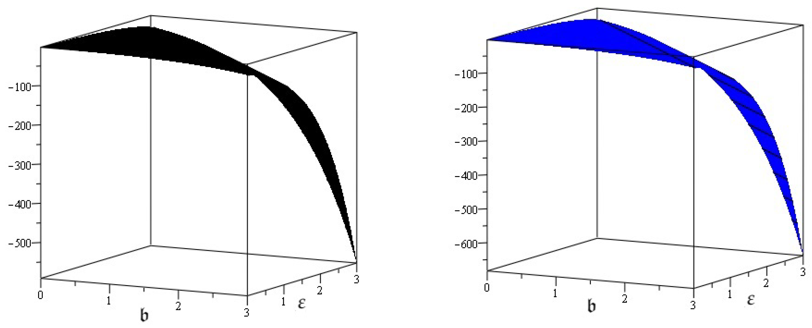
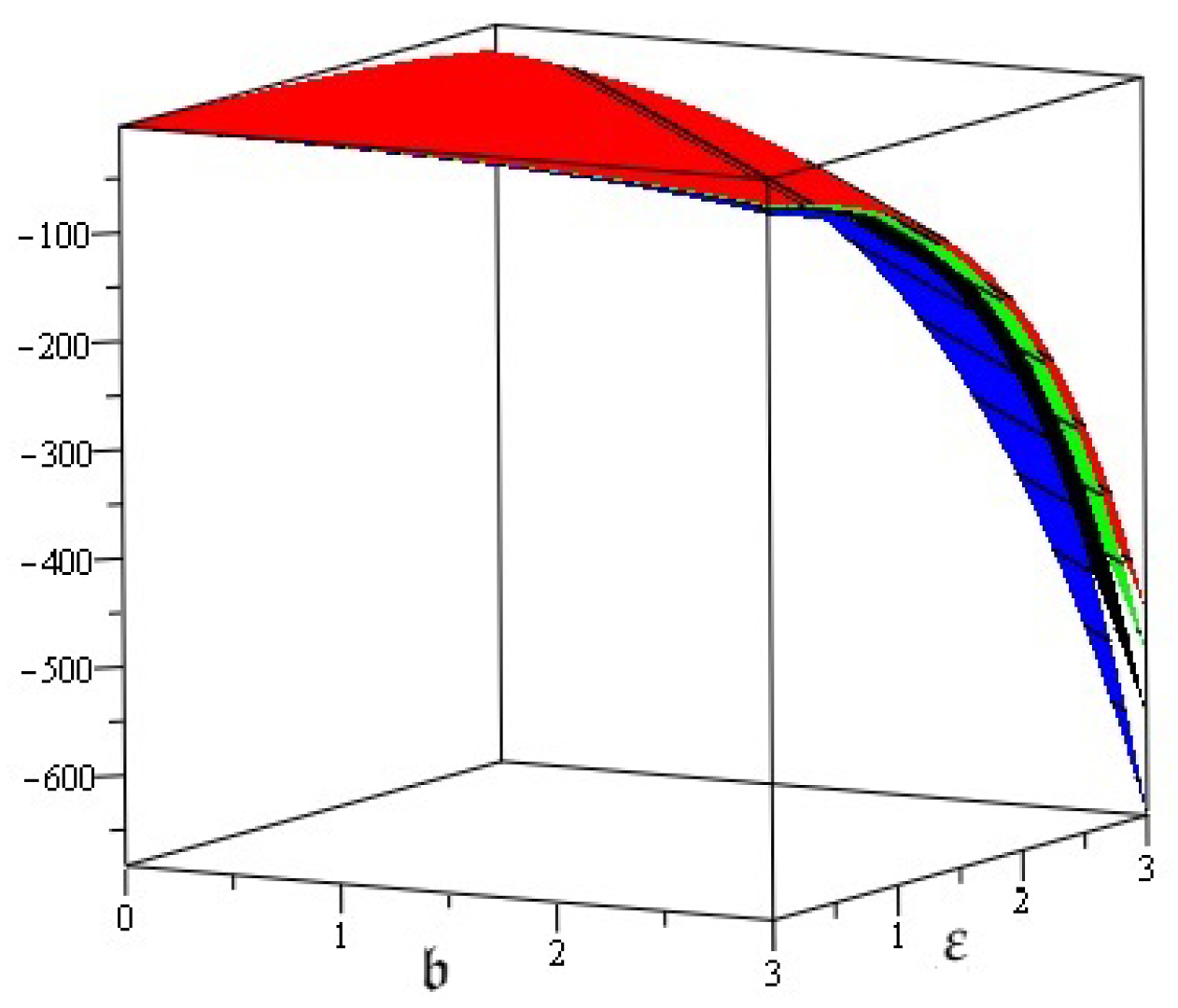
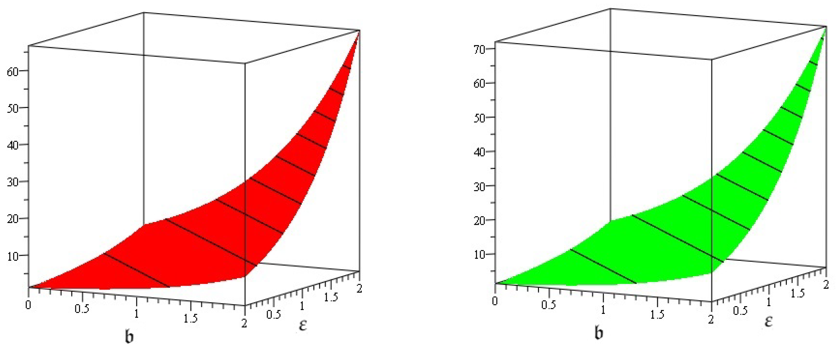
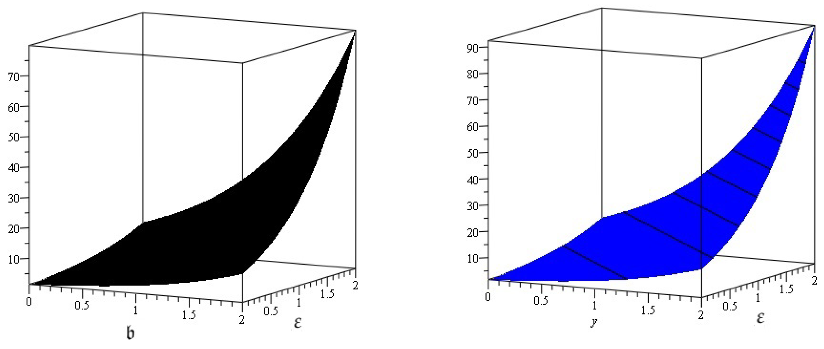
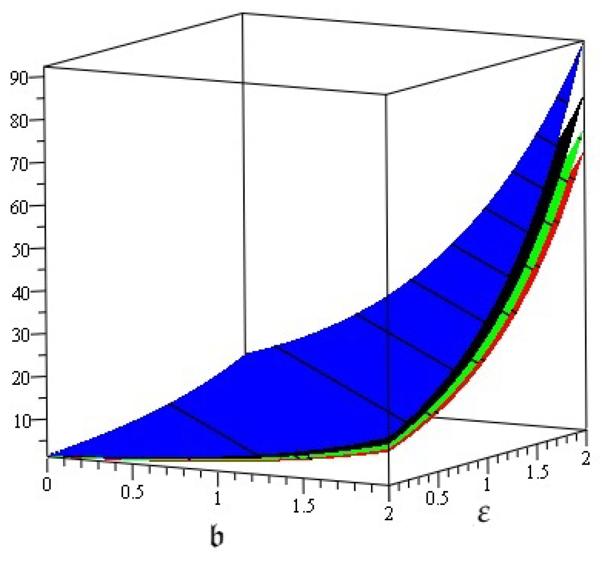
In this section, we analysis the solution-figures of problem which have been investigated by applying homotopy perturbation transformation method and the variational iterative transformation method in the sense of Caputo-Fabrizio. Figure 1, represents the three-dimensional solution-figures for variables of example 1 at fractional order and , respectively in Figure 2 at and . It is observed that homotopy perturbation transformation method and the variational iterative transformation method solution-figures are identical and close contact with each other. In Figure 3, show that the different fractional order graph of ℘. In similar way in Figure 4 represents the three-dimensional solution-figures for variables of example 1 at fractional order and , respectively in Figure 5 at and . In Figure 6, show that the different fractional order graph of ℘. The same graphs of the suggested methods are attained and confirmed the applicability of the present techniques. In Figure 7, Figure 8 and Figure 9, the homotopy perturbation transformation method and the variational iterative transformation method solutions are plotted in three dimensional at fractional-order and of example 1. The convergence phenomenon of the fractional-solutions towards integer-solution is observed. The same accuracy is achieved by using the present techniques.
9. Conclusions
This paper used the homotopy perturbation transform methodology and the variational iterative transform method to provide numerical fractional-order solutions for a non-linear system of the unsteady flow of a polytropic gas, which is widely employed in applied mathematics as a challenge for spatial effects. The procedures provide a succession of convergent findings in physical models. The findings of this research are predicted to be beneficial in the analysis of complex non-linear physical issues in the future. These strategies have extremely basic and clear computations. As a solution, we may deduce that these approaches can be applied to a wide range of non-linear fractional-order systems of PDEs.
Author Contributions
Conceptualization, N.I.; Data curation, T.B.; Formal analysis, M.A., N.I. and T.B.; Funding acquisition, T.B.; Investigation, M.A.; Methodology, N.I.; Project administration, T.B.; Software, N.I.; Validation, T.B.; Visualization, M.A. and T.B.; Writing—original draft, M.A. and N.I.; Writing—review and editing, N.I. and T.B. All authors have read and agreed to the published version of the manuscript.
Funding
This research received no external funding.
Institutional Review Board Statement
Not applicable.
Informed Consent Statement
Not applicable.
Data Availability Statement
Not applicable.
Conflicts of Interest
The authors declare no conflict of interest.
References
- Sabatier, J.A.T.M.J.; Agrawal, O.P.; Machado, J.T. Advances in Fractional Calculus; Springer: Dordrecht, The Netherlands, 2007; Volume 4, No. 9. [Google Scholar]
- Atangana, A.; Baleanu, D. Caputo–Fabrizio Derivative Applied to Groundwater Flow within Confined Aquifer. J. Eng. Mech. 2017, 143, 4016005. [Google Scholar] [CrossRef]
- Abbas, M.I. Controllability and Hyers-Ulam stability results of initial value problems for fractional differential equations via generalized proportional-Caputo fractional derivative. Miskolc Math. Notes 2021, 22, 491–502. [Google Scholar] [CrossRef]
- Akdemir, A.O.; Butt, S.I.; Nadeem, M.; Ragusa, M.A. New General Variants of Chebyshev Type Inequalities via Generalized Fractional Integral Operators. Mathematics 2021, 9, 122. [Google Scholar] [CrossRef]
- Alshabanat, A.; Samet, B. A numerical study of a coupled system of fractional differential equations. Filomat 2020, 34, 2585–2600. [Google Scholar] [CrossRef]
- Rezapour, S.; Iqbal, M.Q.; Hussain, A.; Zada, A.; Etemad, S. Fixed Point and Endpoint Theories for Two Hybrid Fractional Differential Inclusions with Operators Depending on an Increasing Function. J. Funct. Spaces 2021, 2021, 4512223. [Google Scholar] [CrossRef]
- Sidhardh, S.; Patnaik, S.; Semperlotti, F. Geometrically non-linear response of a fractional-order nonlocal model of elasticity. Int. J. Non-linear Mech. 2020, 125, 103529. [Google Scholar] [CrossRef]
- Amin, R.; Senu, N.; Hafeez, M.B.; Arshad, N.I.; Ahmadian, A.; Salahshour, S.; Sumelka, W. A Computational AlgorithmL for the numerical solution of non-linear fractional integral equations. Fractals 2022, 30, 2240030. [Google Scholar]
- Patnaik, S.; Sidhardh, S.; Semperlotti, F. Geometrically non-linear analysis of nonlocal plates using fractional calculus. Int. J. Mech. Sci. 2020, 179, 105710. [Google Scholar] [CrossRef]
- Shah, R.; Khan, H.; Baleanu, D.; Kumam, P.; Arif, M. A semi-analytical method to solve family of Kuramoto–Sivashinsky equations. J. Taibah Univ. Sci. 2020, 14, 402–411. [Google Scholar] [CrossRef]
- Khan, H.; Shah, R.; Kumam, P.; Arif, M. Analytical Solutions of Fractional-Order Heat and Wave Equations by the Natural Transform Decomposition Method. Entropy 2019, 21, 597. [Google Scholar] [CrossRef] [Green Version]
- Shah, R.; Khan, H.; Kumam, P.; Arif, M.; Baleanu, D. Natural Transform Decomposition Method for Solving Fractional-Order Partial Differential Equations with Proportional Delay. Mathematics 2019, 7, 532. [Google Scholar] [CrossRef] [Green Version]
- Khan, H.; Shah, R.; Baleanu, D.; Kumam, P.; Arif, M. Analytical Solution of Fractional-Order Hyperbolic Telegraph Equation, Using Natural Transform Decomposition Method. Electronics 2019, 8, 1015. [Google Scholar] [CrossRef] [Green Version]
- Shah, R.; Khan, H.; Mustafa, S.; Kumam, P.; Arif, M. Analytical Solutions of Fractional-Order Diffusion Equations by Natural Transform Decomposition Method. Entropy 2019, 21, 557. [Google Scholar] [CrossRef] [PubMed] [Green Version]
- Madani, M.; Fathizadeh, M.; Khan, Y.; Yildirim, A. On the coupling of the homotopy perturbation method and Laplace transformation. Math. Comput. Model. 2011, 53, 1937–1945. [Google Scholar] [CrossRef]
- Khan, Y.; Wu, Q. Homotopy perturbation transform method for non-linear equations using He’s polynomials. Comput. Math. Appl. 2011, 61, 1963–1967. [Google Scholar] [CrossRef] [Green Version]
- Morales-Delgado, V.F.; Gómez-Aguilar, J.F.; Yépez-Martínez, H.; Baleanu, D.; Jiménez, R.E.; Olivares-Peregrino, V.H. Laplace homotopy analysis method for solving linear partial differential equations using a fractional derivative with and without kernel singular. Adv. Differ. Equ. 2016, 2016, 1. [Google Scholar] [CrossRef] [Green Version]
- Li, Y.; Nohara, B.T.; Liao, S. Series solutions of coupled Van der Pol equation by means of homotopy analysis method. J. Math. Phys. 2010, 51, 63517. [Google Scholar] [CrossRef] [Green Version]
- Shah, R.; Khan, H.; Baleanu, D. Fractional Whitham–Broer–Kaup Equations within Modified Analytical Approaches. Axioms 2019, 8, 125. [Google Scholar] [CrossRef] [Green Version]
- Iqbal, N.; Yasmin, H.; Ali, A.; Bariq, A.; Al-Sawalha, M.M.; Mohammed, W.W. Numerical Methods for Fractional-Order Fornberg-Whitham Equations in the Sense of Atangana-Baleanu Derivative. J. Funct. Spaces 2021, 2021, 2197247. [Google Scholar] [CrossRef]
- Iqbal, N.; Wu, R. Pattern formation by fractional cross-diffusion in a predator-prey model with Beddington-DeAngelis type functional response. Int. J. Mod. Phys. 2019, 33, 1950296. [Google Scholar] [CrossRef]
- Iqbal, N.; Yasmin, H.; Rezaiguia, A.; Kafle, J.; Almatroud, A.O.; Hassan, T.S. Analysis of the Fractional-Order Kaup–Kupershmidt Equation via Novel Transforms. J. Math. 2021, 2021, 2567927. [Google Scholar] [CrossRef]
- Huebner, K.H.; Dewhirst, D.L.; Smith, D.E.; Byrom, T.G. The Finite Element Method for Engineers; John Wiley & Sons: Hoboken, NJ, USA, 2001. [Google Scholar]
- Smith, G.D.; Smith, G.D.; Smith, G.D.S. Numerical Solution of Partial Differential Equations: Finite Difference Methods; Oxford University Press: Oxford, UK, 1985. [Google Scholar]
- Keskin, Y.; Oturanc, G. Reduced Differential Transform Method for Partial Differential Equations. Int. J. Nonlinear Sci. Numer. Simul. 2009, 10, 741–750. [Google Scholar] [CrossRef]
- Gupta, P.K. Approximate analytical solutions of fractional Benney–Lin equation by reduced differential transform method and the homotopy perturbation method. Comput. Math. Appl. 2011, 61, 2829–2842. [Google Scholar] [CrossRef] [Green Version]
- Mohammed, W.W.; Albosaily, S.; Iqbal, N.; El-Morshedy, M. The effect of multiplicative noise on the exact solutions of the stochastic Burgers’ equation. Waves Random Complex Media 2021, 1–13. [Google Scholar] [CrossRef]
- Veeresha, P.; Prakasha, D.G.; Baskonus, H.M. An efficient technique for a fractional-order system of equations describing the unsteady flow of a polytropic gas. Pramana 2019, 93, 1–13. [Google Scholar] [CrossRef]
- Klebanov, I.; Panov, A.; Ivanov, S.; Maslova, O. Group analysis of dynamics equations of self-gravitating polytropic gas. Commun. Nonlinear Sci. Numer. Simul. 2017, 59, 437–443. [Google Scholar] [CrossRef]
- Moradpour, H.; Abri, A.; Ebadi, H. Thermodynamic behavior and stability of Polytropic gas. Int. J. Mod. Phys. D 2016, 25, 1650014. [Google Scholar] [CrossRef] [Green Version]
- Matinfar, M.; Saeidy, M. Homotopy analysis method for solving the equation governing the unsteady flow of a polytropic gas. World Appl. Sci. J. 2010, 9, 980–983. [Google Scholar]
- Maitama, S. Exact solution of equation governing the unsteady flow of a polytropic gas using the natural decomposition method. Appl. Math. Sci. 2014, 8, 3809–3823. [Google Scholar] [CrossRef]
- He, J.-H. Homotopy perturbation technique. Comput. Methods Appl. Mech. Eng. 1999, 178, 257–262. [Google Scholar] [CrossRef]
- He, J.-H. Application of homotopy perturbation method to non-linear wave equations. Chaos Solitons Fractals 2005, 26, 695–700. [Google Scholar] [CrossRef]
- Das, S.; Gupta, P.K. An Approximate Analytical Solution of the Fractional Diffusion Equation with Absorbent Term and External Force by Homotopy Perturbation Method. Z. Naturforschung A 2010, 65, 182–190. [Google Scholar] [CrossRef]
- Yildirim, A. An Algorithm for Solving the Fractional Nonlinear Schrödinger Equation by Means of the Homotopy Perturbation Method. Int. J. Nonlinear Sci. Numer. Simul. 2009, 10, 445–450. [Google Scholar] [CrossRef]
- Yang, X.-J. A new integral transform method for solving steady heat-transfer problem. Therm. Sci. 2016, 20, 639–642. [Google Scholar] [CrossRef] [Green Version]
- He, J. A new approach to non-linear partial differential equations. Commun. Nonlinear Sci. Numer. Simul. 1997, 2, 230–235. [Google Scholar] [CrossRef]
- He, J.-H.; Wu, X.-H. Variational iteration method: New development and applications. Comput. Math. Appl. 2007, 54, 881–894. [Google Scholar] [CrossRef] [Green Version]
- Wazwaz, A.-M. The variational iteration method for analytic treatment for linear and non-linear ODEs. Appl. Math. Comput. 2009, 212, 120–134. [Google Scholar]
- Wazwaz, A.-M. The variational iteration method for rational solutions for KdV, K(2,2), Burgers, and cubic Boussinesq equations. J. Comput. Appl. Math. 2007, 207, 18–23. [Google Scholar] [CrossRef] [Green Version]
- Caputo, M.; Fabrizio, M. On the singular kernels for fractional derivatives. some applications to partial differential equations. Progr. Fract. Differ. Appl. 2021, 7, 1–4. [Google Scholar]
- Ahmad, S.; Ullah, A.; Akgül, A.; De la Sen, M. A Novel Homotopy Perturbation Method with Applications to Nonlinear Fractional Order KdV and Burger Equation with Exponential-Decay Kernel. J. Funct. Spaces 2021, 2021, 8770488. [Google Scholar] [CrossRef]
Figure 1.
The solution graph of the HPTM/VITM of of Example 1 at (left) and (right).

Figure 2.
The solution graph of the HPTM/VITM of of Example 1 at (left) and (right).

Figure 3.
The graph of the HPTM/VITM of of Example 1 at various fractional orders.

Figure 4.
The solution graph of the HPTM/VITM of of Example 1 at (left) and (right).

Figure 5.
The solution graph of the HPTM/VITM of of Example 1 at (left) and (right).

Figure 6.
The solution graph of the HPTM/VITM of of Example 1 at different fractional orders.

Figure 7.
The solution graph of the HPTM/VITM of of Example 1 at (left) and (right).

Figure 8.
The solution graph of the HPTM/VITM of of Example 1 at (left) and (right).

Figure 9.
The solution graphof the HPTM/VITM of of example 1 at different fractional orders.

Publisher’s Note: MDPI stays neutral with regard to jurisdictional claims in published maps and institutional affiliations. |
© 2022 by the authors. Licensee MDPI, Basel, Switzerland. This article is an open access article distributed under the terms and conditions of the Creative Commons Attribution (CC BY) license (https://creativecommons.org/licenses/by/4.0/).
Share and Cite
MDPI and ACS Style
Alesemi, M.; Iqbal, N.; Botmart, T. Novel Analysis of the Fractional-Order System of Non-Linear Partial Differential Equations with the Exponential-Decay Kernel. Mathematics 2022, 10, 615. https://doi.org/10.3390/math10040615
AMA Style
Alesemi M, Iqbal N, Botmart T. Novel Analysis of the Fractional-Order System of Non-Linear Partial Differential Equations with the Exponential-Decay Kernel. Mathematics. 2022; 10(4):615. https://doi.org/10.3390/math10040615
Chicago/Turabian StyleAlesemi, Meshari, Naveed Iqbal, and Thongchai Botmart. 2022. "Novel Analysis of the Fractional-Order System of Non-Linear Partial Differential Equations with the Exponential-Decay Kernel" Mathematics 10, no. 4: 615. https://doi.org/10.3390/math10040615
Note that from the first issue of 2016, this journal uses article numbers instead of page numbers. See further details here.