
PFVAE: A Planar Flow-Based Variational Auto-Encoder Prediction Model for Time Series Data


1
Artificial Intelligence College, Beijing Technology and Business University, Beijing 100048, China
2
China Light Industry Key Laboratory of Industrial Internet and Big Data, Beijing Technology and Business University, Beijing 100048, China
*
Author to whom correspondence should be addressed.
Mathematics 2022, 10(4), 610; https://doi.org/10.3390/math10040610
Submission received: 7 January 2022
/
Revised: 11 February 2022
/
Accepted: 14 February 2022
/
Published: 16 February 2022
(This article belongs to the Special Issue Mathematical Method and Application of Machine Learning)
Abstract
:Prediction based on time series has a wide range of applications. Due to the complex nonlinear and random distribution of time series data, the performance of learning prediction models can be reduced by the modeling bias or overfitting. This paper proposes a novel planar flow-based variational auto-encoder prediction model (PFVAE), which uses the long- and short-term memory network (LSTM) as the auto-encoder and designs the variational auto-encoder (VAE) as a time series data predictor to overcome the noise effects. In addition, the internal structure of VAE is transformed using planar flow, which enables it to learn and fit the nonlinearity of time series data and improve the dynamic adaptability of the network. The prediction experiments verify that the proposed model is superior to other models regarding prediction accuracy and proves it is effective for predicting time series data.
1. Introduction
Time series data refer to a sequence of sampling arranged in chronological order [1]. With the development of sensors, information communication, and computer storage technology, the time series data collected have become more abundant. Time series data prediction has become one of the key research directions in artificial intelligence, widely found in traffic flow [2], air pollution [3,4,5], anomaly detection [6,7,8], etc. The parameters of time series models can be used for identification methods [9,10,11,12,13], such as hierarchical algorithms [14,15,16,17,18].
At present, the prediction methods of time series data can be roughly divided into three categories: statistical methods, machine-learning methods, and deep learning algorithms [19,20]. Statistical methods include generalized linear prediction model [21], seasonal gray prediction model [22], Markov prediction method [23], Gaussian process model [24], etc. These models have clear mathematical forms and are easy to understand, while they require the data’s prior knowledge. Moreover, it is difficult to describe the complex nonlinearity.
In contrast, machine-learning methods with parameter self-learning and nonlinear adaptation are more suitable for time series data. The most widely used machine-learning methods include artificial neural network (ANN) [25], support vector regression (SVR) [26], integrated moving average autoregressive model (ARIMA) [27], etc. These models are easy to implement, but they cannot fit complex nonlinear relationships due to insufficient parameters [28,29].
The deep learning method has been popular in artificial intelligence in recent years. It can learn effective feature representations from extensive input data and has robust learning and predictive capabilities [30,31,32]. Recurrent neural network (RNN) [33] in deep learning and its variant forms of long short-term memory network (LSTM) [34] and gated recurrent unit (GRU) [35] has been widely used in the field of time series data prediction. In addition, many advanced network structures have been studied, such as bidirectional long short-term memory network (BiLSTM) [36], bidirectional gated recurrent unit (BiGRU) [37], convolutional neural network-long short-term memory network (CNN-LSTM) [38], convolutional long short-term memory network (ConvLSTM) [39], and Bayesian long short-term memory network (BayesLSTM) [40,41]. BiLSTM and BiGRU can improve the model’s learning power by considering the complete past and future contextual information; ConvLSTM improves the LSTM network’s ability by introducing convolution calculations. BayesLSTM improves LSTM based on variational reasoning theory, replacing fixed-value weights and deviations with optimizable and sampled distributions, which enhances the anti-noise ability and robustness of the model.
Although the abovementioned RNN-based methods have been widely used in time series data prediction, its modeling is still an opening problem due to the complex nonlinear relationship and random distribution of time series data. The remaining paper is as follows. Section 2 summarizes the related works and Section 3 introduces the model proposed, named PFVAE, in detail. Section 4 describes the experimental results to support the model’s effectiveness; finally, Section 5 summarizes and suggests future work.
2. Related Works
The machine-learning model is one of the popular prediction methods in time series data, such that Fi-John Chang et al. [42] used the self-organizing mapping method to extract spatiotemporal features of series data; Gholamreza Goudarzi et al. [43] used an artificial neural network, and Wenbo Liu et al. [44] used support vector regression with different kernel functions to predict the daily average concentration of PM2.5 in Beijing; Shihab Ahmad Shahriar et al. [45] evaluated autoregressive integrated moving average (ARIMA)-artificial neural network (ANN), ARIMA-support vector machine (SVM), and principal component regression (PCR) along with decision tree (DT) and CatBoost deep learning model for the prediction. In practice, machine-learning methods are unsuitable for big time series data prediction with complex nonlinearities because they will fail to give enough performance.
Compared with the classical machine-learning model, deep learning networks have powerful modeling capabilities, can extract potential information, and are widely used in time series data prediction. Xue-Bo Jin et al. [46] proposed a deep hybrid model with a serial two-layer decomposition structure to predict the future power load. Agga, Ali, et al. [47] proposed two models, CNN-LSTM and ConvLSTM, to predict the power generation of photovoltaic power plants in four different time ranges from 1 day to 7 days; Luo, Xianglong, et al. [48] proposed a structural deformation prediction model based on the time convolutional network (TCN), which uses one-dimensional expansion causal convolution to reduce model parameters and obtain long-term memory of time series. Although deep learning methods have strong learning capabilities, the prediction performance is not high enough since a large amount of data causes the learning efficiency of neural networks to be low.
Auto-encoder is a data compression algorithm that can compress and decompress data to reduce noise and complex information interference. Therefore, it has attracted more attention in time series prediction. Yi-Wei Lu et al. [49] proposed a model based on an auto-encoder gated recurrent unit (AE-GRU), where an auto-encoder (AE) extracts important features from raw data and a gated recurrent unit (GRU) selects information to predict the remaining service life. Xinghan Xu et al. [50] proposed a LSTM auto-encoder multi-task predictor to predict air quality in multiple locations. Ki-Su Kim et al. [51] proposed a deep learning model combining a denoising auto-encoder and convolutional LSTM to predict global ocean weather. Thanongsak Xayasouk et al. [52] used LSTM and deep auto-encoder (DAE) to predict the concentration of fine particles.
With the increase of research on auto-encoders, many special auto-encoders have appeared. Variational auto-encoder (VAE) can describe an observation in latent space with a probability distribution, which has been widely used in image and classification and has been gradually applied in time series prediction. Xiaosong Zhu et al. [53] proposed a long-term deformation prediction model for arch dams based on VAE and time attention-based long short-term memory (TALSTM) network. To improve the accuracy of equipment health prediction, Yanfang Yang et al. [54] proposed a neural network prediction model combining VAE and time convolutional network (TCN), which uses VAE to reduce the dimensionality, extracts the hidden information in the original data, reconstructs high-quality sample data, and then uses TCN to mine the internal connection in the long sequence of information.
In the above research, VAE only uses Gaussian approximation, which makes it challenging to simulate the complex time series data. On the other hand, normalizing flow is a tool for calculating complicated distribution. Aditya Arie Nugraha et al. [55] combined the normalizing flows with the VAE method to establish a latent variable model called GF-VAE for speech spectrogram modeling and enhancement; Philippe Esling et al. [56] proposed an audio synthesizer control formula by variational auto-encoder (VAE) and normalized stream. Henter, Gustav Eje et al. [57] proposed a model for probability, generation, and controllable motion data based on normalizing flows with MoGlow. The model is used to generate motion data sequences from normalizing flows so that it cannot only describe the distribution with high complexity but can use accurate maximum likelihood for effective training; Ho, YH et al. [58] built an end-to-end learning image compression system based on a novel flow model Augmented Normalizing Flows (ANF) and stacked with multiple Variational Auto-encoders (VAEs) is built.
The research above illustrates the high modeling ability of normalizing flows for nonlinear relationships. This paper uses VAE as the time series data predictor with normalizing flows to model the complex posterior distribution of time series data, which guarantees the robustness of the network to noise and improves its ability to model complex nonlinear relationships. The main contributions of this research are as follows:
- (1)
- VAE with LSTM is designed as a time series data predictor to learn the long- and short-term dependencies of time series data. Compared with the prediction networks [34,35,36,37,38,39,40,48,53], the proposed VAE model can effectively learn the relation and extract representative information of time series and improve the computational efficiency of the model. Moreover, it has sufficient robustness to noise and prevents overfitting.
- (2)
- Based on the Planar flow, this paper reforms the internal structure of VAE, improves the modeling ability of complex posterior approximation, enables it to learn and process time series data with more complex characteristics, and improves the nonlinearity and dynamic adaptability of the network.
3. Method
3.1. Variational Auto-Encoder (VAE)
When neural networks are used in time series prediction and image processing, they often need to receive a large amount of input information, usually containing useless or less valuable data, making it difficult for neural networks to learn. Therefore, we must compress a large amount of input data, extract representative information from the data, reduce the amount of input information, and put the reduced information into the neural network for learning so that the neural network will be easier to learn.
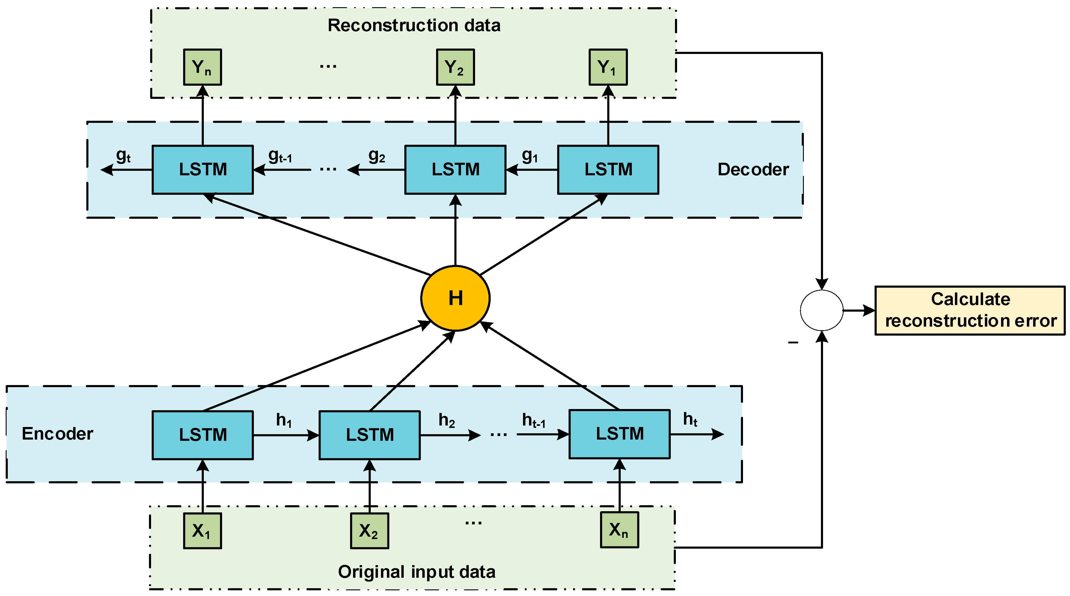
An auto-encoder is a data compression algorithm in which the data compression and decompression functions are data-related, lossy, and automatically learned from samples. In most cases where auto-encoders are mentioned, compression and decompression functions are implemented through neural networks. In this research, we used LSTM as the encoder and decoder to realize the compression and reconstruction process of the input data. The proposed prediction auto-encoder is shown in Figure 1.
In Figure 1, represents the original input data, and represents the hidden state passed in the encoder and decoder, respectively, H is the encoding vector output by the encoder, which means the essence of the original input data, and represents the reconstructed data through the decoder. The model’s error is the difference between the reference input and the reconstructed data, defined as the reconstruction error. The auto-encoder uses the mean square error (MSE) as the loss function to calculate the reconstruction error. The loss function is defined as follows:
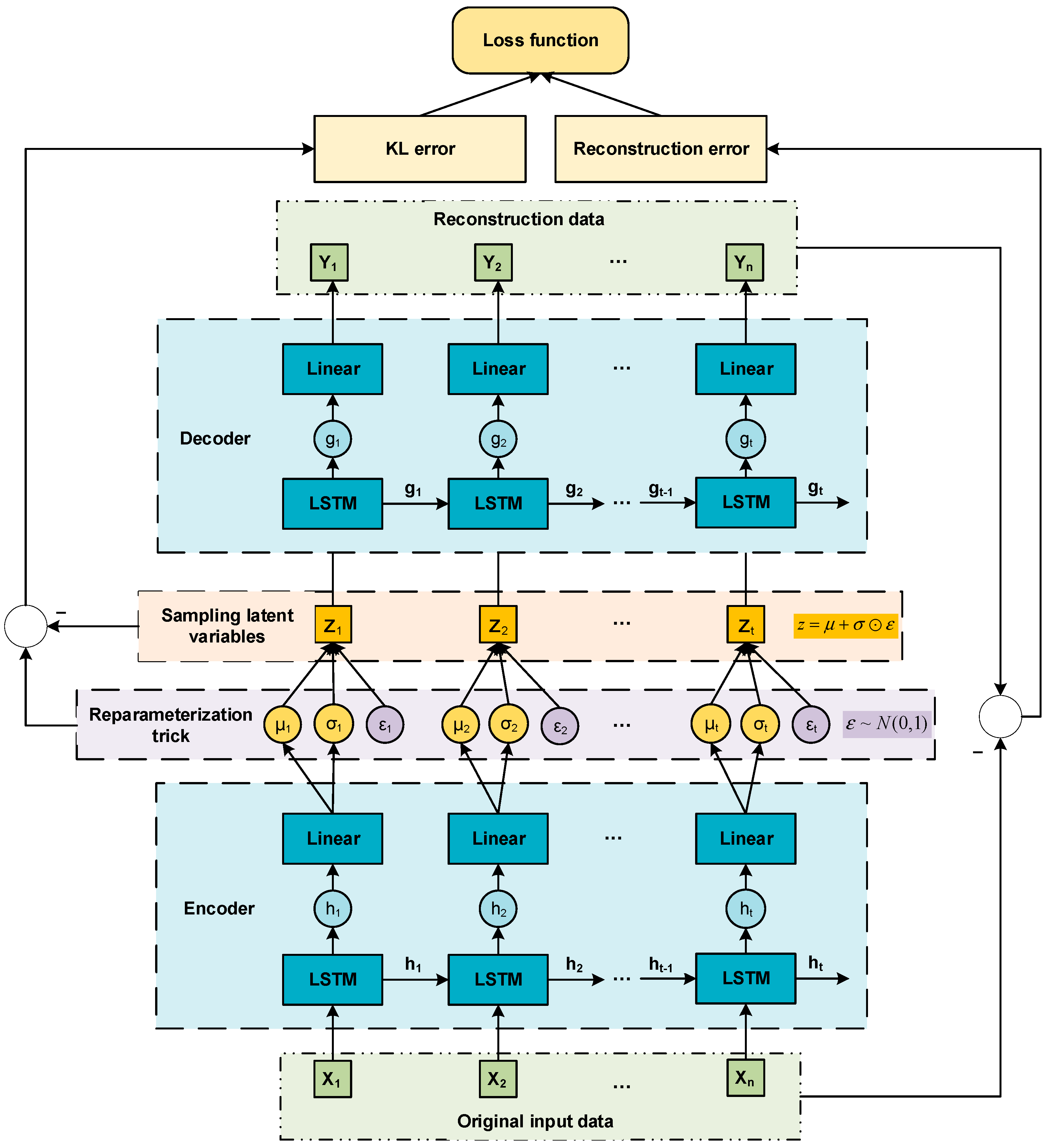
where is the total number of samples in the dataset, is the i-th reference value in the test set, and is the reconstructed value obtained by the model. Then we develop the auto-encoder in Figure 1 to VAE by variational inference [59], shown in Figure 2.
In Figure 2, and are the mean and variance obtained by the encoder after encoding the input data; is the parameter required for reparameterization, ; is the latent variable sampled.
It can be seen from Figure 2 that the loss function of VAE described as (2) includes: (1) the reconstruction error between the reference input data and reconstructed data; (2) the Kullback–Leibler divergence error (KL error) caused by the encoder sampling.
where and , stands for the element-wise product.
The optimization mechanism of the loss function of VAE can be understood as an adversarial learning process for and :
When the reconstructed data of VAE differs from the reference data, the mean and variance will be adjusted to fit the sampled data, thus is changed to improve the quality of the reconstructed data.
3.2. VAE Based on Normalizing Flows
3.2.1. Planar Flow: One of the Normalizing Flows
To optimize in Formula (2), we must find a distribution that is the same with posterior distribution as the input data. Still, the general Gaussian distribution cannot fit a sufficiently complex posterior distribution. Therefore, we embed normalizing flows into the VAE model.
The normalizing flows describe the transformation of probability density through a reversible mapping sequence. The initial density “flow” passes through the reversible mapping sequence, repeatedly applying the variable transformation rules [60].
By optimizing this series of distributions, a simple Gaussian distribution can be changed into a complex actual posterior distribution.
Specifically, given a reversible mapping: , use it to transform the latent variable into a new variable , therefore the distribution of the new variable is:
Formula (3) is the Jacobian matrix of invertible functions by the chain rule (inverse function theorem). It is possible to construct the complex density by synthesizing several simple mappings and applying Formula (3) in turn. For the random variable with the distribution of , the transformation chain is sequentially used, and after times, the density obtained is:
and,
In this way, it is not necessary to explicitly calculate , but only the initial distribution and the mapped Jacobian matrix. Normalizing flows need to find an invertible mapping function that the Jacobian matrix can be operated on efficiently. Here we used one of the normalizing flows called the Planar flow.
Planar flow is defined as a function of the following form:
where and are vectors (called scale and weight here), is a scalar (deviation) to be set by learning, is the activation function.
For Planar flow, the determinant of the Jacobian can be calculated in time by relying on the matrix determinant lemma:
3.2.2. VAE Based on Planar Flow
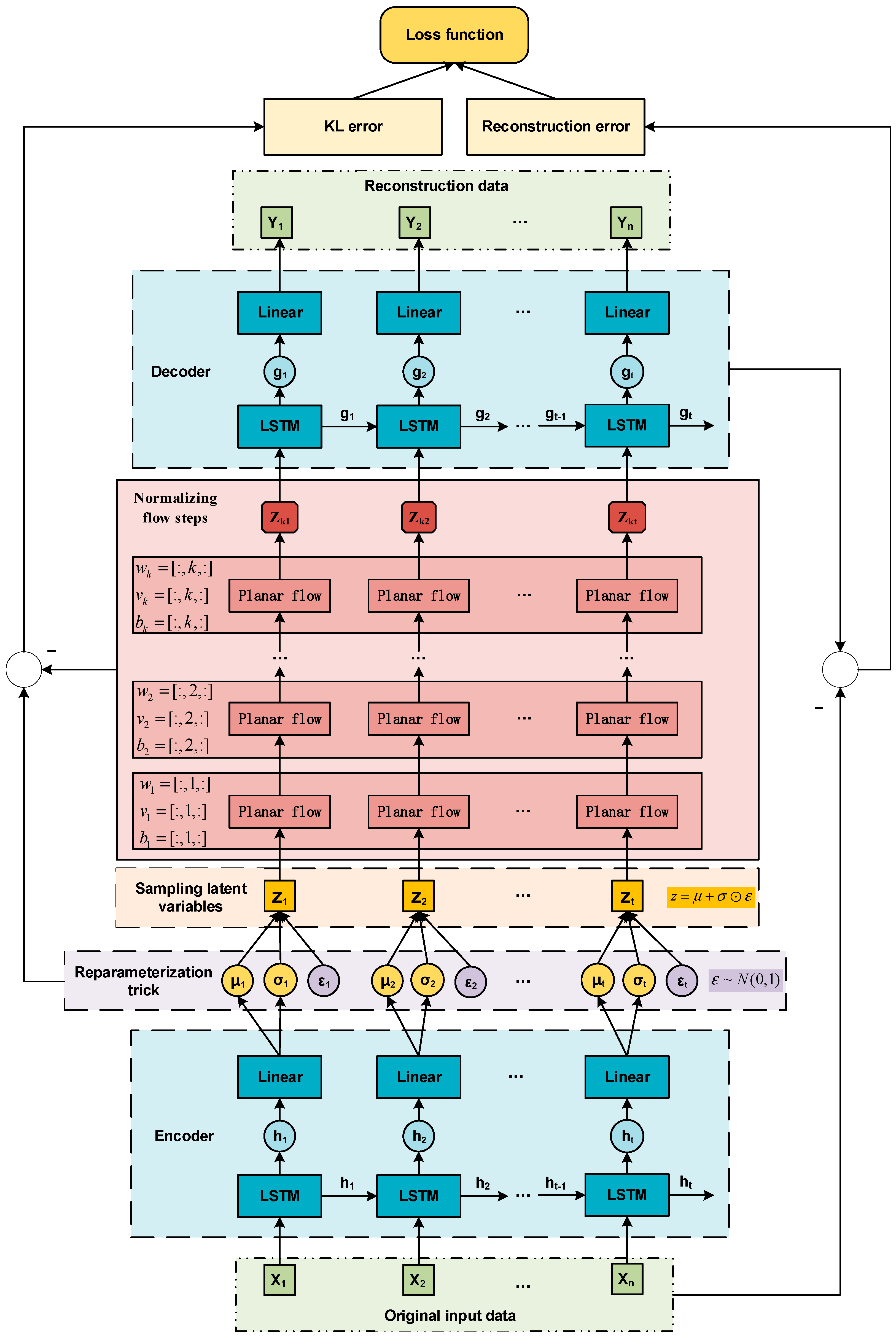
We used the Planar flow of length to parameterize the approximate posterior distribution of the encoder in the VAE. The proposed PFVAE prediction model structure is shown in Figure 4. , and are the weights, scales, and deviations of Planar flow; is a latent variable with a complex distribution obtained by the Planar flow posterior.
In the case of applying Planar flow , Equation (9) can be written as the expectation of the initial distribution:
Normalizing flows and free energy circles can be used in any variational optimization scheme. For variational inference, we used a deep neural network to build an inference model from the observation to the initial density and the parameter of the flow to create a mapping. The complete optimization goal is written as:
The Planar flow is used as the posterior to fit the complicated posterior distribution. It enables the VAE prediction model to learn and process time series data with complex characteristics and improves the network’s degree of nonlinearity and dynamic adaptability. The loss function of PFVAE is shown in Formula (11):
With the Planar flow method, the output of the encoder is sampled from a more complex distribution than the Gaussian distribution. This makes the reconstructed output of the decoder more robust to noise, improves the reconstruction of data with a high degree of nonlinearity, and improves the dynamic adaptability of the prediction model.
The specific iterative calculation process of our proposed PFVAE prediction model is shown below:
- (1)
- The input data is encoded by the encoder to obtain and .
- (2)
- Using the reparameterization technique and sampling the latent variable , we get , .
- (3)
- Planar flow is applied to obtain latent variables with a complex distribution .
- (4)
- The latent variables are entered into the decoder to obtain reconstructed data .
- (5)
- Calculate loss function and optimize the model.
4. Experimental Results and Discussions
4.1. Experiment Setup and Evaluation Indicators
The experiments were performed on a desktop computer equipped with an AMD R7-5800 processor, 4.0 GHz, and 16 GB of RAM by PyTorch to build a VAE-LSTM network model based on the Planar flow. This consists of a LSTM network for the encoder and decoder with hidden neural units set to 24 and used the Adam algorithm to perform supervised learning. Its learning rate was set to 0.01, and 100 epochs were trained. The prediction steps were 24.
We used 80% of the data as the model’s training set and the remaining 20% as the test set. The Z-score method shown in (12) was used for standardizing the input data.
where represents the input data, represents the mean value of the observation data, represents the variance of the observation data.
In the experiment, we compared the prediction performance with the other seven models, LSTM [34], GRU [35], BiLSTM [36], BiGRU [37], TCN [48], CNN-LSTM [38], ConvLSTM [39], BayesLSTM [40], and VAE [53], under the same parameters and the same dataset.
In order to evaluate the predictive performance of different models, six evaluation indicators were used, including root mean square error (RMSE), mean absolute error (MAE), symmetric mean fundamental percentage error (SMAPE), mean square error (MSE), Pearson correlation coefficient (R), and goodness-of-fit (R2). The calculation formulas of these six evaluation indicators are shown in Formulas (13)–(18):
where is the total number of samples in the dataset, is the actual in the test set, is the average value of the actual value, is the i-th prediction, and is the average value of the prediction.
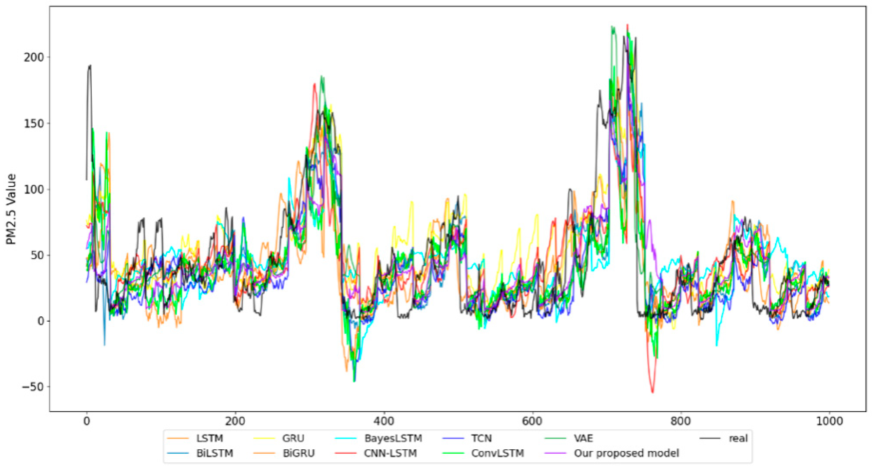
4.2. PM2.5 Prediction
This study used the PM2.5 concentration data in Beijing, China to carry out verification experiments. With the continuous development of the global economy, people are paying more and more attention to the ecological environment. Air pollution is one of the most urgent environmental pollution problems. The PM2.5 is a particulate matter with a diameter of less than 2.5 μm, an essential indicator for measuring and controlling the degree of air pollution. As air quality is affected by various factors such as meteorological factors and human factors, the changes of PM 2.5 time series data are highly nonlinear and are disturbed by noise, which is a challenging problem in forecasting.
The sampling time in the experiment was from 1 January 2017 to 31 December 2019, with a sampling frequency of 1 h. In Figure 5, we show part of the prediction results of each model.
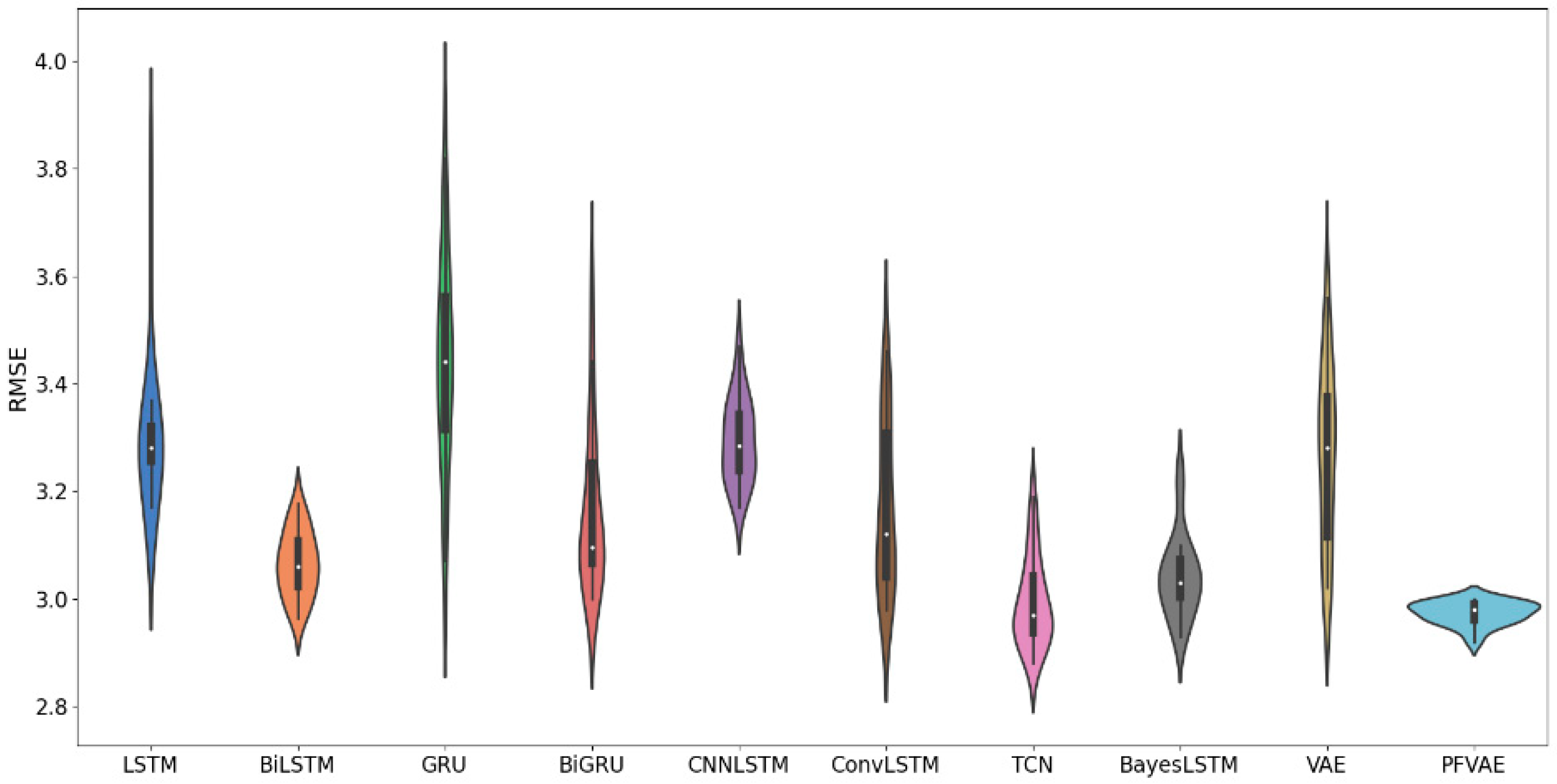
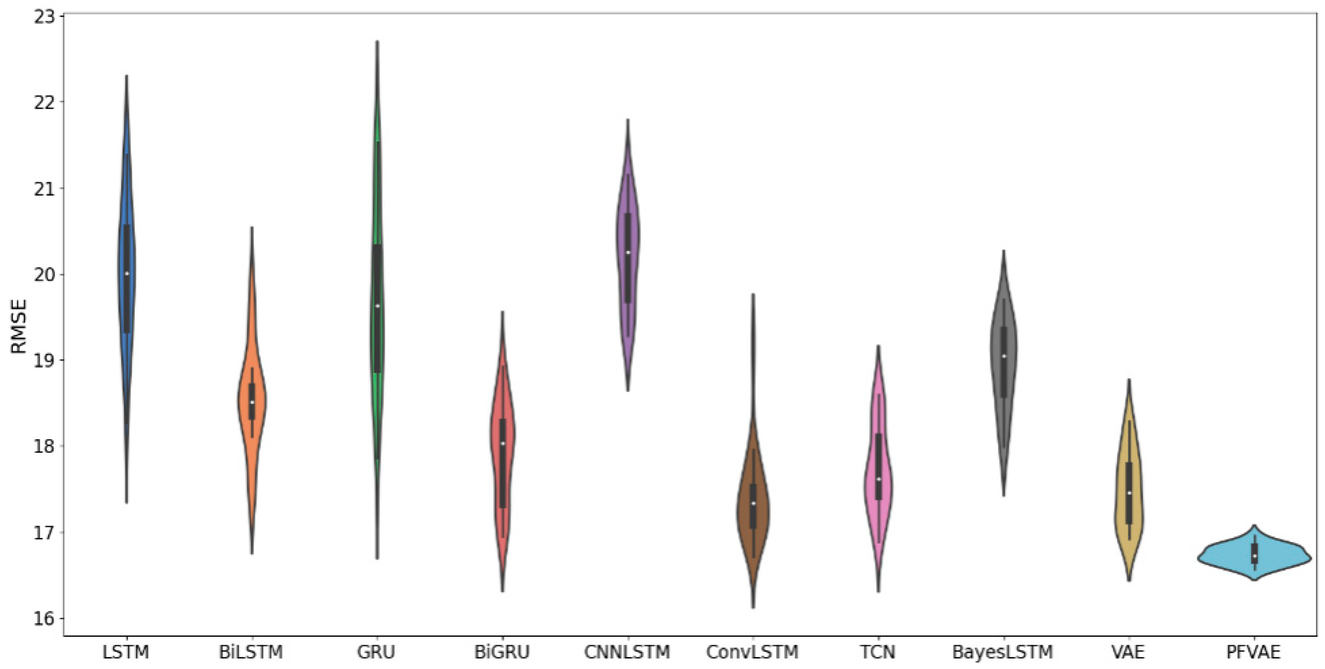
To validate the effectiveness of the proposed method, we repeated each model independently with the same dataset 20 times and recorded its RMSE values to ensure the objectivity of the results. The statistical results are shown in Figure 6.
As shown in Figure 6, our proposed model (PFVAE) has the minor error range, the most uniform and concentrated distribution, and the smallest average error of the model, which maintains high accuracy and stability compared to other models.
It can be seen from Table 1 that our proposed model has the lowest RMSE, MAE, SMAPE, and MSE and the highest R and R2. RMSE, MAE, SMAPE, MSE, R and R2 were 24.45, 17.07, 51.29, 598.13, 0.65 and 0.42, respectively. Compared with the other seven models, the RMSE of our PFVAE model improved by 26.9%, 6.0%, 15.5%, 9.2% 15.0%, 7.2%, 8.6%, 18.5%, and 5.3%, respectively; MAE improved by 30.5%, 3.1%, 20.1%, 4.1%, 16.8%, 5.7%, 7.5%, 26.2%, and 3.6%, respectively. As for SMAPE, the prediction performance of the PFVAE model proposed improved by 23.5%, 3.3%, 17.3%, 7.9%, 14.4%, 7.9%, 16.4%, 26.1%, and 3.3%, respectively; and MSE, 46.5%, 11.5%, 28.5%, 17.5%, 27.8%, 13.9%, 16.5%, 33.6%, and 10.4%, respectively. Moreover, the maximum R-value and R2-value of the proposed PFVAE model represent the best fit between the predicted and observed values. The above experimental data show that our proposed model is better than other models in terms of prediction accuracy and result fit, which proves the applicability of this model in the field of time series prediction.
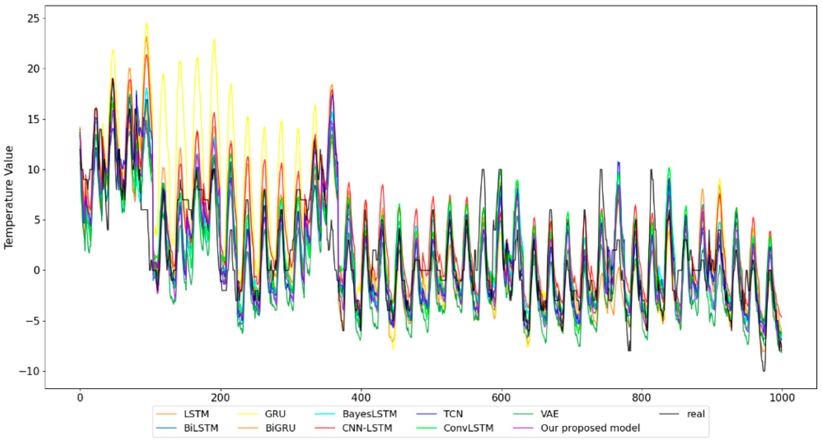
4.3. Temperature Prediction
This study used the temperature data from Haidian District, Beijing, China, to conduct verification experiments. As we know, changes in atmospheric temperature are closely related to human production and life. The atmospheric temperature significantly impacts human travel, social development, and the ecological environment. Therefore, accurate prediction of atmospheric temperature has essential application prospects in people’s daily life.
Figure 7 shows part of the prediction results. The sampling time was from 1 January 2017 to 31 December 2019, with a sampling frequency of 1 h. The statistical results are shown in Figure 8.
Figure 8 shows that the proposed model (PFVAE) obtained the highest accuracy and stability compared to other models. It can be seen from Table 2 that compared with the other seven models, RMSE improved by 12.2%, 3.9%, 30.5%, 9.3%, 12.5%, 9.5%, 3.9%, 3.3%, and 14.3%, respectively; MAE, though the same as TCN, improved compared to others by 11.2%, 7.2%, 33.7%, 10.9%, 13.0%, 13.0%, 4.3%, and 15.7%, respectively. As with SMAPE, the prediction performance of the PFVAE model improved by 5.1%, 4.8%, 14.5%, 5.5%, 11.7%, 6.2%, 1.3%, 3.7%, and 13.9%, respectively; and MSE, 23.3%, 7.5%, 51.8%, 17.7%, 23.7%, 14.8%, 7.6%, 6.5%, and 26.7%, respectively. Moreover, the maximum R-value and R2-value of the proposed PFVAE model represent the best fit between the predicted and observed values.
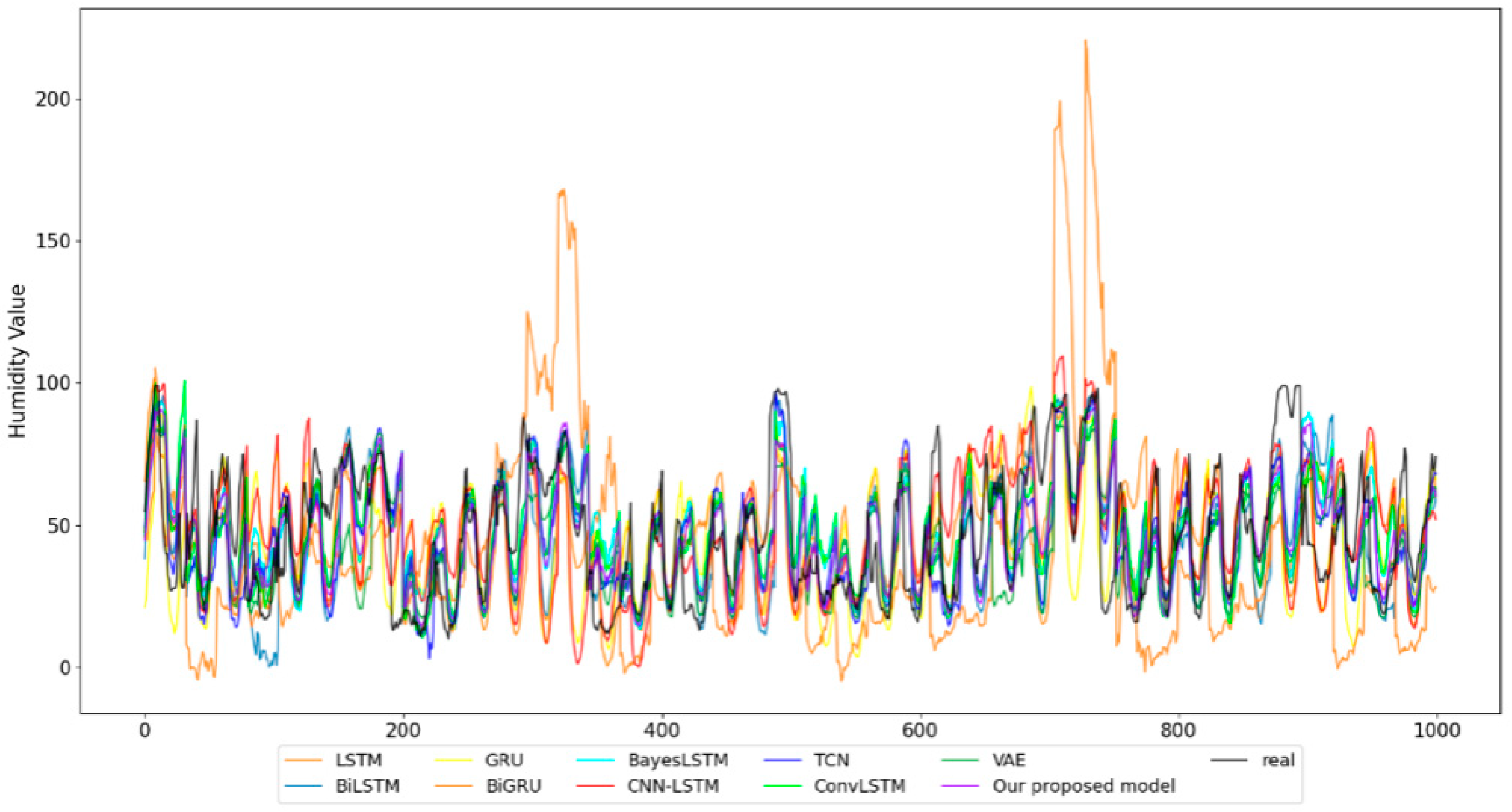
4.4. Humidity Prediction
In this study, we used the humidity data of Haidian District, Beijing, China to carry out verification experiments. The sampling time was from 1 January 2017 to 31 December 2019, with a sampling frequency of 1 h. In Figure 9, we show part of the prediction results of each model.
As shown in Figure 10, our proposed model (PFVAE) has a minor error fluctuation range, the most uniform and concentrated distribution, and the smallest average error of the models.
It can be seen from Table 3 that compared with the other seven models, our PFVAE model improved RMSE by 19.0%, 8.5%, 19.6%, 5.7%, 20.4%, 0.7%, 4.1%, 2.1%, and 7.6%, respectively; MAE improved by 20.4%, 4.3%, 19.3%, 2.5%, 21.8%, 0.6%, 3.2%, 2.1%, and 9.4%, respectively. As with SMAPE, though it is almost the same as ConvLSTM, it increased by 20.7%, 9.7%, 25.5%, 9.8%, 27.2%, 5.6%, 3.1%, and 9.4%; and MSE, 34.4%, 16.3%, 35.4%, 16.3%,36.6%, 1.4%, 8.0%, 4.2%, and 14.8%, respectively. Moreover, the maximum R-value and R2-value of the proposed PFVAE model represent the best fit between the predicted and observed values. The results show that our proposed model is better than other models in terms of prediction accuracy and result fit.
5. Summary and Future Work
It is challenging to learn and fit the prediction model due to the high nonlinearity and complex random distribution of time series data. This paper proposed a novel VAE prediction model based on Planar flow, which uses LSTM as the encoder and decoder and designs VAE as a time series data predictor, using Planar flow to transform the internal structure of VAE to learn the time series data with complex characteristics. Through verification experiments on a variety of time series datasets and the multiple evaluation indicators such as RMSE, MAE, SMAPE, MSE, R, and R2, our proposed model is superior to other models in terms of prediction accuracy. The proposed prediction approaches of time series models in the paper can combine other parameter estimation algorithms [61,62,63,64,65,66,67,68] with studying the parameter identification problems of linear and nonlinear systems with different disturbances [69,70,71,72,73,74,75,76,77]. The proposed prediction approach can build the soft sensor models and prediction models based on the time series data and can be applied to other fields [78,79,80,81,82,83,84,85,86], such as signal processing and engineering application systems [87,88,89,90,91].
In future work, we will further verify the effectiveness of our proposed time series forecasting model. Meanwhile, we will explore other normalizing flows to transform our proposed prediction model.
Author Contributions
Conceptualization, X.-B.J. and W.-T.G.; methodology, X.-B.J. and W.-T.G.; software, W.-T.G.; validation, X.-B.J. and W.-T.G.; formal analysis, J.-L.K.; investigation, Y.-T.B. and T.-L.S.; resources, X.-B.J. and J.-L.K.; data curation, W.-T.G., Y.-T.B. and T.-L.S.; writing—original draft preparation, X.-B.J. and W.-T.G.; writing—review and editing, X.-B.J. and W.-T.G.; visualization, W.-T.G.; supervision, J.-L.K., Y.-T.B. and T.-L.S.; project administration, X.-B.J. and J.-L.K.; funding acquisition, X.-B.J. All authors have read and agreed to the published version of the manuscript.
Funding
This work was supported in part by the National Natural Science Foundation of China, No. 62006008, 62173007, 61903009.
Data Availability Statement
Not applicable.
Conflicts of Interest
The authors declare no conflict of interest.
References
- Kim, J.; Moon, N. A deep bidirectional similarity learning model using dimensional reduction for multivariate time series clus-tering. Multimed. Tools Appl. 2021, 80, 34269–34281. [Google Scholar] [CrossRef]
- Qiao, Y.; Wang, Y.; Ma, C.; Yang, J. Short-term traffic flow prediction based on 1DCNN-LSTM neural network structure. Mod. Phys. Lett. B 2020, 35, 2150042. [Google Scholar] [CrossRef]
- Kong, T.; Choi, D.; Lee, G.; Lee, K. Air Pollution Prediction Using an Ensemble of Dynamic Transfer Models for Multivariate Time Series. Sustainability 2021, 13, 1367. [Google Scholar] [CrossRef]
- Jin, X.; Yang, N.; Wang, X.; Bai, Y.; Su, T.; Kong, J. Integrated Predictor Based on Decomposition Mechanism for PM2.5 Long-Term Prediction. Appl. Sci. 2019, 9, 4533. [Google Scholar] [CrossRef] [Green Version]
- Jin, X.B.; Yang, N.X.; Wang, X.Y.; Bai, Y.T.; Su, T.L.; Kong, J.L. Deep hybrid model based on EMD with classification by frequency characteristics for long-term air quality prediction. Mathematics 2020, 8, 214. [Google Scholar] [CrossRef] [Green Version]
- Ji, Z.; Gong, J.; Feng, J. A Novel Deep Learning Approach for Anomaly Detection of Time Series Data. Sci. Program. 2021, 2021, 6636270. [Google Scholar] [CrossRef]
- Du, S.; Li, T.; Yang, Y.; Horng, S.-J. Multivariate time series forecasting via attention-based encoder–decoder framework. Neurocomputing 2020, 388, 269–279. [Google Scholar] [CrossRef]
- Jin, X.B.; Yu, X.H.; Wang, X.Y.; Bai, Y.T.; Su, T.L.; Kong, J.L. Deep learning predictor for sustainable precision agriculture based on internet of things system. Sustainability 2020, 12, 1433. [Google Scholar] [CrossRef] [Green Version]
- Ding, F.; Chen, T. Combined parameter and output estimation of dual-rate systems using an auxiliary model. Automatica 2004, 40, 1739–1748. [Google Scholar] [CrossRef]
- Ding, F.; Chen, T. Parameter estimation of dual-rate stochastic systems by using an output error method. IEEE Trans. Autom. Control 2005, 50, 1436–1441. [Google Scholar] [CrossRef]
- Ding, F.; Shi, Y.; Chen, T. Auxiliary model-based least-squares identification methods for Hammerstein output-error systems. Syst. Control Lett. 2007, 56, 373–380. [Google Scholar] [CrossRef]
- Zhou, Y.; Ding, F. Modeling Nonlinear Processes Using the Radial Basis Function-Based State-Dependent Autoregressive Models. IEEE Signal Process. Lett. 2020, 27, 1600–1604. [Google Scholar] [CrossRef]
- Zhou, Y.; Zhang, X.; Ding, F. Partially-coupled nonlinear parameter optimization algorithm for a class of multivariate hybrid models. Appl. Math. Comput. 2021, 414, 126663. [Google Scholar] [CrossRef]
- Zhou, Y.; Zhang, X.; Ding, F. Hierarchical Estimation Approach for RBF-AR Models with Regression Weights Based on the Increasing Data Length. IEEE Trans. Circuits Syst. II Express Briefs 2021, 68, 3597–3601. [Google Scholar] [CrossRef]
- Ding, F.; Zhang, X.; Xu, L. The innovation algorithms for multivariable state-space models. Int. J. Adapt. Control Signal Process. 2019, 33, 1601–1618. [Google Scholar] [CrossRef]
- Ding, F.; Liu, G.; Liu, X.P. Parameter estimation with scarce measurements. Automatica 2011, 47, 1646–1655. [Google Scholar] [CrossRef]
- Liu, Y.; Ding, F.; Shi, Y. An efficient hierarchical identification method for general dual-rate sampled-data systems. Automatica 2014, 50, 962–970. [Google Scholar] [CrossRef]
- Zhang, X.; Ding, F. Optimal Adaptive Filtering Algorithm by Using the Fractional-Order Derivative. IEEE Signal Process. Lett. 2022, 29, 399–403. [Google Scholar] [CrossRef]
- Wang, B.; Kong, W.; Zhao, P. An air quality forecasting model based on improved convnet and RNN. Soft Comput. 2021, 25, 9209–9218. [Google Scholar] [CrossRef]
- Shi, Z.; Bai, Y.; Jin, X.; Wang, X.; Su, T.; Kong, J. Parallel deep prediction with covariance intersection fusion on non-stationary time series. Knowl.-Based Syst. 2021, 211, 106523. [Google Scholar] [CrossRef]
- Cholianawati, N.; Cahyono, W.E.; Indrawati, A.; Indrajad, A. Linear Regression Model for Predicting Daily PM2.5 Using VIIRS-SNPP and MODIS-Aqua AOT. In IOP Conference Series: Earth and Environmental Science; IOP Publishing: Bristol, UK, 2019; Volume 303. [Google Scholar]
- Zhou, W.; Wu, X.; Ding, S.; Ji, X.; Pan, W. Predictions and mitigation strategies of PM2.5 concentration in the Yangtze River Delta of China based on a novel nonlinear seasonal grey model. Environ. Pollut. 2021, 276, 116614. [Google Scholar] [CrossRef] [PubMed]
- Li, T.; Ma, J.; Lee, C. Markov-Based Time Series Modeling Framework for Traffic-Network State Prediction under Various External Conditions. J. Transp. Eng. Part A Syst. 2020, 146, 04020042. [Google Scholar] [CrossRef]
- Jang, J.; Shin, S.; Lee, H.; Moon, I.C. Forecasting the Concentration of Particulate Matter in the Seoul Metropolitan Area Using a Gaussian Process Model. Sensors 2020, 20, 3845. [Google Scholar] [CrossRef] [PubMed]
- Abraham, E.R.; Mendes dos Reis, J.G.; Vendrametto, O.; Oliveira Costa Neto, P.L.D.; Carlo Toloi, R.; Souza, A.E.D.; Oliveira Morais, M.D. Time series prediction with artificial neural networks: An analysis using Brazilian soybean production. Agriculture 2020, 10, 475. [Google Scholar] [CrossRef]
- Quan, Q.; Hao, Z.; Xifeng, H.; Jingchun, L. Research on water temperature prediction based on improved support vector regression. Neural Comput. Appl. 2020, 1–10. [Google Scholar] [CrossRef]
- Guo, N.; Chen, W.; Wang, M.; Tian, Z.; Jin, H. Applying an Improved Method Based on ARIMA Model to Predict the Short-Term Electricity Consumption Transmitted by the Internet of Things (IoT). Wirel. Commun. Mob. Comput. 2021, 2021, 6610273. [Google Scholar] [CrossRef]
- Wen, C.; Liu, S.; Yao, X.; Peng, L.; Li, X.; Hu, Y.; Chi, T. A novel spatiotemporal convolutional long short-term neural network for air pollution prediction. Sci. Total Environ. 2018, 654, 1091–1099. [Google Scholar] [CrossRef]
- Jin, X.B.; Yang, N.X.; Wang, X.Y.; Bai, Y.T.; Su, T.L.; Kong, J.L. Hybrid deep learning predictor for smart agriculture sensing based on empirical mode decomposition and gated recurrent unit group model. Sensors 2020, 20, 1334. [Google Scholar] [CrossRef] [Green Version]
- Kong, J.; Wang, H.; Wang, X.; Jin, X.; Fang, X.; Lin, S. Multi-stream Hybrid Architecture Based on Cross-level Fusion Strategy for Fine-grained Crop Species Recognition in Precision Agriculture. Comput. Electron. Agric. 2021, 185, 106134. [Google Scholar] [CrossRef]
- Kong, J.; Yang, C.; Wang, J.; Wang, X.; Zuo, M.; Jin, X.; Lin, S. Deep-stacking network approach by multisource data mining for hazardous risk identification in IoT-based intelligent food management systems. Comput. Intell. Neurosci. 2021, 2021, 1194565. [Google Scholar] [CrossRef]
- Jin, X.B.; Zheng, W.Z.; Kong, J.L.; Wang, X.Y.; Zuo, M.; Zhang, Q.C.; Lin, S. Deep-Learning Temporal Predictor via Bidirectional Self-attentive Encoder-decoder framework for IOT-based Environmental Sensing in Intelligent Greenhouse. Agriculture 2021, 11, 802. [Google Scholar] [CrossRef]
- Connor, J.T.; Martin, R.D.; Atlas, L.E. Recurrent neural networks and robust time series prediction. IEEE Trans. Neural Netw. 1994, 5, 240–254. [Google Scholar] [CrossRef] [PubMed] [Green Version]
- Choi, H.-M.; Kim, M.-K.; Yang, H. Abnormally high water temperature prediction using LSTM deep learning model. J. Intell. Fuzzy Syst. 2021, 40, 8013–8020. [Google Scholar] [CrossRef]
- Becerra-Rico, J.; Aceves-Fernández, M.A.; Esquivel-Escalante, K.; Pedraza-Ortega, J.C. Airborne particle pollution predictive model using Gated Recurrent Unit (GRU) deep neural networks. Earth Sci. Inform. 2020, 13, 821–834. [Google Scholar] [CrossRef]
- Abduljabbar, R.L.; Dia, H.; Tsai, P.W. Unidirectional and Bidirectional LSTM Models for Short-Term Traffic Prediction. J. Adv. Transp. 2021, 2021, 5589075. [Google Scholar] [CrossRef]
- Chen, W.; Qi, W.; Li, Y.; Zhang, J.; Zhu, F.; Xie, D.; Ru, W.; Luo, G.; Song, M.; Tang, F. Ultra-Short-Term Wind Power Prediction Based on Bidirectional Gated Recurrent Unit and Transfer Learning. Front. Energy Res. 2021, 9, 808116. [Google Scholar] [CrossRef]
- Elmaz, F.; Eyckerman, R.; Casteels, W.; Latré, S.; Hellinckx, P. CNN-LSTM architecture for predictive indoor temperature modeling. Build. Environ. 2021, 206, 108327. [Google Scholar] [CrossRef]
- Wang, W.; Mao, W.; Tong, X.; Xu, G. A Novel Recursive Model Based on a Convolutional Long Short-Term Memory Neural Network for Air Pollution Prediction. Remote Sens. 2021, 13, 1284. [Google Scholar] [CrossRef]
- Jin, X.B.; Yu, X.H.; Su, T.L.; Yang, D.N.; Bai, Y.T.; Kong, J.L.; Wang, L. Distributed deep fusion predictor for multi-sensor system based on causality entropy. Entropy 2021, 23, 219. [Google Scholar] [CrossRef]
- Jin, X.-B.; Zheng, W.-Z.; Kong, J.-L.; Wang, X.-Y.; Bai, Y.-T.; Su, T.-L.; Lin, S. Deep-Learning Forecasting Method for Electric Power Load via Attention-Based Encoder-Decoder with Bayesian Optimization. Energies 2021, 14, 1596. [Google Scholar] [CrossRef]
- Chang, F.J.; Chang, L.C.; Kang, C.C.; Wang, Y.S.; Huang, A. Explore Spatio-temporal PM2.5 features in northern Taiwan using machine learning techniques. Sci. Total Environ. 2020, 736, 139656. [Google Scholar] [CrossRef] [PubMed]
- Goudarzi, G.; Hopke, P.K.; Yazdani, M. Forecasting PM2.5 concentration using artificial neural network and its health effects in Ahvaz, Iran. Chemosphere 2021, 283, 131285. [Google Scholar] [CrossRef] [PubMed]
- Liu, W.; Liang, S.; Yu, Q. PM2.5 concentration prediction based on pseudo-F statistic feature selection algorithm and support vector regression. In IOP Conference Series: Earth and Environmental Science; IOP Publishing: Bristol, UK, 2020; Volume 569. [Google Scholar] [CrossRef]
- Shahriar, S.A.; Kayes, I.; Hasan, K.; Hasan, M.; Islam, R.; Awang, N.R.; Hamzah, Z.; Rak, A.E.; Salam, M.A. Potential of Arima-ann, Arima-SVM, dt and catboost for atmospheric PM2.5 forecasting in bangladesh. Atmosphere 2021, 12, 100. [Google Scholar] [CrossRef]
- Jin, X.B.; Wang, H.X.; Wang, X.Y.; Bai, Y.T.; Su, T.L.; Kong, J.L. Deep-learning prediction model with serial two-level decomposition based on Bayesian optimization. Complexity 2020, 2020, 4346803. [Google Scholar] [CrossRef]
- Agga, A.; Abbou, A.; Labbadi, M.; El Houm, Y. Short-term self consumption PV plant power production forecasts based on hybrid CNN-LSTM, ConvLSTM models. Renew. Energy 2021, 177, 101–112. [Google Scholar] [CrossRef]
- Luo, X.; Gan, W.; Wang, L.; Chen, Y.; Ma, E. A Deep Learning Prediction Model for Structural Deformation Based on Temporal Convolutional Networks. Comput. Intell. Neurosci. 2021, 2021, 8829639. [Google Scholar] [CrossRef]
- Lu, Y.W.; Hsu, C.Y.; Huang, K.C. An autoencoder gated recurrent unit for remaining useful life prediction. Processes 2020, 8, 1155. [Google Scholar] [CrossRef]
- Xu, X.; Yoneda, M. Multitask Air-Quality Prediction Based on LSTM-Autoencoder Model. IEEE Trans. Cybern. 2019, 51, 2577–2586. [Google Scholar] [CrossRef]
- Kim, K.S.; Lee, J.B.; Roh, M.I.; Han, K.M.; Lee, G.H. Prediction of Ocean Weather Based on Denoising AutoEncoder and Convolutional LSTM. J. Mar. Sci. Eng. 2020, 8, 805. [Google Scholar] [CrossRef]
- Xayasouk, T.; Lee, H.; Lee, G. Air Pollution Prediction Using Long Short-Term Memory (LSTM) and Deep Autoencoder (DAE) Models. Sustainability 2020, 12, 2570. [Google Scholar] [CrossRef] [Green Version]
- Shu, X.; Bao, T.; Li, Y.; Gong, J.; Zhang, K. VAE-TALSTM: A temporal attention and variational autoencoder-based long short-term memory framework for dam displacement prediction. Eng. Comput. 2021, 1–16. [Google Scholar] [CrossRef]
- Yang, Y.; Yu, B.; Wang, W. Research on equipment health prediction technology based on edge computing and VAE-TCN. Procedia Comput. Sci. 2021, 183, 100–106. [Google Scholar] [CrossRef]
- Nugraha, A.A.; Sekiguchi, K.; Yoshii, K. A flow-based deep latent variable model for speech spectrogram modeling and en-hancement. IEEE/ACM Trans. Audio Speech Lang. Process. 2020, 28, 1104–1117. [Google Scholar] [CrossRef]
- Esling, P.; Masuda, N.; Bardet, A.; Despres, R.; Chemla-Romeu-Santos, A. Flow synthesizer: Universal audio synthesizer control with normalizing flowss. Appl. Sci. 2020, 10, 302. [Google Scholar] [CrossRef] [Green Version]
- Henter, G.E.; Alexanderson, S.; Beskow, J. Moglow: Probabilistic and controllable motion synthesis using normalising flows. ACM Trans. Graph. 2020, 39, 1–14. [Google Scholar] [CrossRef]
- Ho, Y.H.; Chan, C.C.; Peng, W.H.; Hang, H.M.; Domański, M. ANFIC: Image Compression Using Augmented Normalizing Flows. IEEE Open J. Circuits Syst. 2021, 2, 613–626. [Google Scholar] [CrossRef]
- Rocca, J. Understanding Variational Autoencoders (VAEs). 2019. Available online: https://towardsdatascience.com/understanding-variational-autoencoders-vaes-f70510919f73 (accessed on 7 December 2021).
- Rezende, D.; Mohamed, S. Variational inference with normalizing flows. In Proceedings of the 32nd International Conference on Machine Learning, Lille, France, 6–11 July 2015. [Google Scholar]
- Ding, F.; Lv, L.; Pan, J.; Wan, X.; Jin, X.-B. Two-stage Gradient-based Iterative Estimation Methods for Controlled Autoregressive Systems Using the Measurement Data. Int. J. Control Autom. Syst. 2019, 18, 886–896. [Google Scholar] [CrossRef]
- Ding, F.; Wang, F.F.; Wu, M.H. Decomposition based least squares iterative identification algorithm for multivariate pseu-do-linear ARMA systems using the data filtering. J. Frankl. Inst. 2017, 354, 1321–1339. [Google Scholar] [CrossRef]
- Zhang, X.; Ding, F. Hierarchical parameter and state estimation for bilinear systems. Int. J. Syst. Sci. 2020, 51, 275–290. [Google Scholar] [CrossRef]
- Zhang, X.; Yang, E.F. State estimation for bilinear systems through minimizing the covariance matrix of the state estimation errors. Int. J. Adapt. Control Signal Process. 2019, 33, 1157–1173. [Google Scholar] [CrossRef]
- Pan, J.; Ma, H.; Zhang, X.; Liu, Q.; Ding, F.; Chang, Y.; Sheng, J. Recursive coupled projection algorithms for multivariable output-error-like systems with coloured noises. IET Signal Process. 2020, 14, 455–466. [Google Scholar] [CrossRef]
- Xu, L.; Ding, F.; Zhu, Q. Decomposition strategy-based hierarchical least mean square algorithm for control systems from the impulse responses. Int. J. Syst. Sci. 2021, 52, 1806–1821. [Google Scholar] [CrossRef]
- Zhang, X.; Xu, L.; Ding, F.; Hayat, T. Combined state and parameter estimation for a bilinear state space system with moving average noise. J. Frankl. Inst. 2018, 355, 3079–3103. [Google Scholar] [CrossRef]
- Pan, J.; Jiang, X.; Wan, X.; Ding, W. A filtering based multi-innovation extended stochastic gradient algorithm for multivariable control systems. Int. J. Control Autom. Syst. 2017, 15, 1189–1197. [Google Scholar] [CrossRef]
- Ding, F.; Liu, G.; Liu, X.P. Partially Coupled Stochastic Gradient Identification Methods for Non-Uniformly Sampled Systems. IEEE Trans. Autom. Control 2010, 55, 1976–1981. [Google Scholar] [CrossRef]
- Ding, F.; Shi, Y.; Chen, T. Performance analysis of estimation algorithms of non-stationary ARMA processes. IEEE Trans. Signal Process. 2006, 54, 1041–1053. [Google Scholar] [CrossRef]
- Wang, Y.; Ding, F.; Wu, M. Recursive parameter estimation algorithm for multivariate output-error systems. J. Frankl. Inst. 2018, 355, 5163–5181. [Google Scholar] [CrossRef]
- Zhang, X.; Ding, F. Adaptive parameter estimation for a general dynamical system with unknown states. Int. J. Robust Nonlinear Control 2020, 30, 1351–1372. [Google Scholar] [CrossRef]
- Zhang, X.; Ding, F.; Xu, L. Recursive parameter estimation methods and convergence analysis for a special class of nonlinear systems. Int. J. Robust Nonlinear Control 2020, 30, 1373–1393. [Google Scholar] [CrossRef]
- Zhang, X.; Ding, F. Recursive parameter estimation and its convergence for bilinear systems. IET Control Theory Appl. 2020, 14, 677–688. [Google Scholar] [CrossRef]
- Xu, L. Separable Multi-innovation Newton Iterative Modeling Algorithm for Multi-frequency Signals Based on the Sliding Measurement Window. Circuits Syst. Signal Process. 2022, 41, 805–830. [Google Scholar] [CrossRef]
- Xu, L. Separable Newton Recursive Estimation Method Through System Responses Based on Dynamically Discrete Measurements with Increasing Data Length. Int. J. Control Autom. Syst. 2022, 20, 432–443. [Google Scholar] [CrossRef]
- Xu, L.; Ding, F.; Yang, E. Auxiliary model multi-innovation stochastic gradient parameter estimation methods for nonlinear sandwich systems. Int. J. Robust Nonlinear Control 2021, 31, 148–165. [Google Scholar] [CrossRef]
- Liu, S.; Ding, F.; Xu, L.; Hayat, T. Hierarchical Principle-Based Iterative Parameter Estimation Algorithm for Dual-Frequency Signals. Circuits Syst. Signal Process. 2019, 38, 3251–3268. [Google Scholar] [CrossRef]
- Wan, L.; Ding, F. Decomposition- and gradient-based iterative identification algorithms for multivariable systems using the mul-ti-innovation theory. Circuits Syst. Signal Process. 2019, 38, 2971–2991. [Google Scholar] [CrossRef]
- Wang, X.; Ding, F. Modified particle filtering-based robust estimation for a networked control system corrupted by impulsive noise. Int. J. Robust Nonlinear Control 2021, 32, 830–850. [Google Scholar] [CrossRef]
- Pan, J.; Li, W.; Zhang, H. Control Algorithms of Magnetic Suspension Systems Based on the Improved Double Exponential Reaching Law of Sliding Mode Control. Int. J. Control Autom. Syst. 2018, 16, 2878–2887. [Google Scholar] [CrossRef]
- Ma, H.; Pan, J.; Ding, F.; Xu, L.; Ding, W. Partially-coupled least squares based iterative parameter estimation for multi-variable out-put-error-like autoregressive moving average systems. IET Control Theory Appl. 2019, 13, 3040–3051. [Google Scholar] [CrossRef]
- Ding, F.; Liu, P.X.; Yang, H. Parameter Identification and Intersample Output Estimation for Dual-Rate Systems. IEEE Trans. Syst. Man Cybern. Part A Syst. Hum. 2008, 38, 966–975. [Google Scholar] [CrossRef]
- Ding, F.; Liu, X.P.; Liu, G. Multiinnovation least squares identification for linear and pseudo-linear regression models. IEEE Trans. Syst. Man Cybern. Part B Cybern. 2010, 40, 767–778. [Google Scholar] [CrossRef]
- Xu, L.; Song, G. A Recursive Parameter Estimation Algorithm for Modeling Signals with Multi-frequencies. Circuits Syst. Signal Process. 2020, 39, 4198–4224. [Google Scholar] [CrossRef]
- Xu, L.; Ding, F.; Wan, L.; Sheng, J. Separable multi-innovation stochastic gradient estimation algorithm for the nonlinear dynamic responses of systems. Int. J. Adapt. Control Signal Process. 2020, 34, 937–954. [Google Scholar] [CrossRef]
- Shu, J.; He, J.; Li, L. MSIS: Multispectral Instance Segmentation Method for Power Equipment. Comput. Intell. Neurosci. 2022, 2022, 2864717. [Google Scholar] [CrossRef] [PubMed]
- Peng, H.; He, W.; Zhang, Y.; Li, X.; Ding, Y.; Menon, V.G.; Verma, S. Covert non-orthogonal multiple access communication assisted by multi-antenna jamming. Phys. Commun. 2022, 52, 101598. [Google Scholar] [CrossRef]
- Hou, J.; Chen, F.; Li, P.; Zhu, Z. Gray-Box Parsimonious Subspace Identification of Hammerstein-Type Systems. IEEE Trans. Ind. Electron. 2021, 68, 9941–9951. [Google Scholar] [CrossRef]
- Zhao, Z.; Zhou, Y.; Wang, X.; Wang, Z.; Bai, Y. Water quality evolution mechanism modeling and health risk assessment based on stochastic hybrid dynamic systems. Expert Syst. Appl. 2022, 193, 116404. [Google Scholar] [CrossRef]
- Chen, Q.; Zhao, Z.; Wang, X.; Xiong, K.; Shi, C. Microbiological predictive modeling and risk analysis based on the one-step kinetic integrated Wiener process. Innovat. Food Sci. Emerg. Technol. 2022, 75, 102912. [Google Scholar] [CrossRef]
Figure 1.
Prediction structure diagram of auto-encoder by LSTM.

Figure 2.
VAE structure diagram.

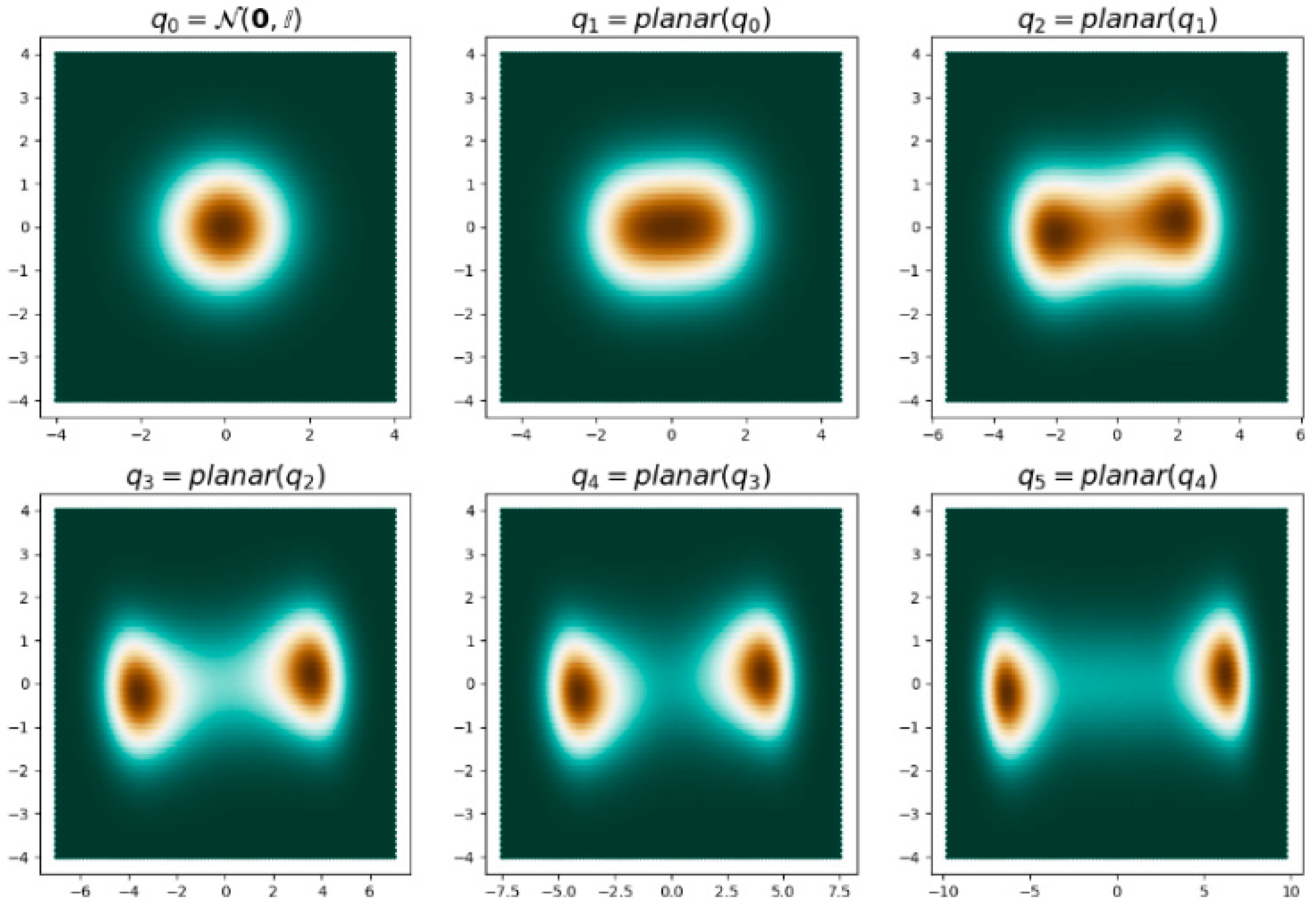
Figure 3.
Applied Planar flow transformation distribution. is the initial unimodal Gaussian distribution, is the bimodal distribution obtained by Planar flow.
Figure 3.
Applied Planar flow transformation distribution. is the initial unimodal Gaussian distribution, is the bimodal distribution obtained by Planar flow.

Figure 4.
PFVAE prediction model structure.

Figure 5.
Plots of prediction results of different models on the PM2.5 dataset.

Figure 6.
RMSE violin plots for each model run 20 times on the PM2.5 dataset.

Figure 7.
Plots of prediction results of different models on temperature datasets.

Figure 8.
RMSE violin plots for each model run 20 times on the temperature dataset.

Figure 9.
Plots of prediction results of different models on the humidity dataset.

Figure 10.
RMSE violin plots for each model run 20 times on the humidity dataset.


Table 1.
Accuracy evaluation of prediction results of each model on the PM2.5 dataset.
| Model | RMSE | MAE | SMAPE | MSE | R | R2 |
|---|---|---|---|---|---|---|
| LSTM [34] | 33.45 | 24.59 | 67.06 | 1119.05 | 0.44 | −0.08 |
| BiLSTM [36] | 26.00 | 17.62 | 53.04 | 676.05 | 0.61 | 0.30 |
| GRU [35] | 28.93 | 21.37 | 62.09 | 836.67 | 0.56 | −0.19 |
| BiGRU [37] | 26.92 | 17.80 | 55.70 | 724.74 | 0.59 | 0.32 |
| CNN-LSTM [38] | 28.78 | 20.52 | 59.94 | 828.56 | 0.52 | 0.20 |
| ConvLSTM [39] | 26.36 | 18.11 | 55.74 | 694.78 | 0.60 | 0.33 |
| TCN [48] | 26.77 | 18.46 | 61.41 | 716.66 | 0.61 | 0.31 |
| BayesLSTM [40] | 30.03 | 23.16 | 69.47 | 901.75 | 0.47 | 0.13 |
| VAE [53] | 25.84 | 17.72 | 53.08 | 667.91 | 0.61 | 0.36 |
| The proposed method | 24.45 | 17.07 | 51.29 | 598.13 | 0.65 | 0.42 |
Table 2.
Accuracy evaluation of prediction results of each model on temperature dataset.
| Model | RMSE | MAE | SMAPE | MSE | R | R2 |
|---|---|---|---|---|---|---|
| LSTM [34] | 3.34 | 2.48 | 33.31 | 11.19 | 0.95 | 0.91 |
| BiLSTM [36] | 3.05 | 2.37 | 33.22 | 9.28 | 0.97 | 0.93 |
| GRU [35] | 4.22 | 3.32 | 37.00 | 17.83 | 0.93 | 0.86 |
| BiGRU [37] | 3.23 | 2.47 | 33.46 | 10.42 | 0.97 | 0.92 |
| CNN-LSTM [38] | 3.35 | 2.53 | 35.81 | 11.25 | 0.96 | 0.91 |
| ConvLSTM [39] | 3.24 | 2.53 | 33.70 | 10.48 | 0.96 | 0.92 |
| TCN [48] | 3.05 | 2.20 | 32.05 | 9.29 | 0.96 | 0.93 |
| BayesLSTM [40] | 3.03 | 2.30 | 32.83 | 9.18 | 0.96 | 0.93 |
| VAE [53] | 3.42 | 2.61 | 36.74 | 11.72 | 0.96 | 0.91 |
| The proposed method | 2.93 | 2.20 | 31.61 | 8.58 | 0.96 | 0.93 |
Table 3.
Accuracy evaluation of prediction results of each model on the humidity dataset.
| Model | RMSE | MAE | SMAPE | MSE | R | R2 |
|---|---|---|---|---|---|---|
| LSTM [34] | 20.47 | 15.74 | 29.78 | 419.13 | 0.62 | 0.31 |
| BiLSTM [36] | 18.12 | 13.08 | 26.15 | 328.19 | 0.72 | 0.46 |
| GRU [35] | 20.63 | 15.53 | 31.70 | 425.68 | 0.66 | 0.30 |
| BiGRU [37] | 17.59 | 12.84 | 26.18 | 309.44 | 0.75 | 0.49 |
| CNN-LSTM [38] | 20.83 | 16.03 | 32.47 | 433.83 | 0.65 | 0.29 |
| ConvLSTM [39] | 16.70 | 12.60 | 23.60 | 279.02 | 0.74 | 0.54 |
| TCN [48] | 17.29 | 12.94 | 25.03 | 299.06 | 0.74 | 0.51 |
| BayesLSTM [40] | 16.94 | 12.80 | 24.37 | 287.02 | 0.73 | 0.53 |
| VAE [53] | 17.96 | 13.83 | 26.06 | 322.71 | 0.71 | 0.47 |
| The proposed method | 16.58 | 12.52 | 23.61 | 274.85 | 0.75 | 0.55 |
Publisher’s Note: MDPI stays neutral with regard to jurisdictional claims in published maps and institutional affiliations. |
© 2022 by the authors. Licensee MDPI, Basel, Switzerland. This article is an open access article distributed under the terms and conditions of the Creative Commons Attribution (CC BY) license (https://creativecommons.org/licenses/by/4.0/).
Share and Cite
MDPI and ACS Style
Jin, X.-B.; Gong, W.-T.; Kong, J.-L.; Bai, Y.-T.; Su, T.-L. PFVAE: A Planar Flow-Based Variational Auto-Encoder Prediction Model for Time Series Data. Mathematics 2022, 10, 610. https://doi.org/10.3390/math10040610
AMA Style
Jin X-B, Gong W-T, Kong J-L, Bai Y-T, Su T-L. PFVAE: A Planar Flow-Based Variational Auto-Encoder Prediction Model for Time Series Data. Mathematics. 2022; 10(4):610. https://doi.org/10.3390/math10040610
Chicago/Turabian StyleJin, Xue-Bo, Wen-Tao Gong, Jian-Lei Kong, Yu-Ting Bai, and Ting-Li Su. 2022. "PFVAE: A Planar Flow-Based Variational Auto-Encoder Prediction Model for Time Series Data" Mathematics 10, no. 4: 610. https://doi.org/10.3390/math10040610
Note that from the first issue of 2016, this journal uses article numbers instead of page numbers. See further details here.