Multi-Stage Multi-Product Production and Inventory Planning for Cold Rolling under Random Yield

Abstract

This paper studies a multi-stage multi-product production and inventory planning problem with random yield derived from the cold rolling process in the steel industry. The cold rolling process has multiple stages, and intermediate inventory buffers are kept between stages to ensure continuous operation. Switching products during the cold rolling process is typically very costly. Backorder costs are incurred for unsatisfied demand while inventory holding costs are incurred for excess inventory. The process also experiences random yield. The objective of the production and inventory planning problem is to minimize the total cost including the switching costs, inventory holding costs, and backorder costs. We propose a stochastic formulation with a nonlinear objective function. Two lower bounds are proposed, which are based on full information relaxation and Jensen’s inequality, respectively. Then, we develop two heuristics from the proposed lower bounds. In addition, we propose a two-stage procedure motivated by newsvendor logic. To verify the performance of the proposed bounds and heuristics, computational tests are conducted on synthetic instances. The results show the efficiency of the proposed bounds and heuristics.

1. Introduction

For the manufacturing system, production and inventory planning is oriented to meet the needs of customers. On the basis of comprehensively considering the production process and inventory management requirements, this planning determines the output of each unit and the inventory strategy of each warehouse so as to reduce production and inventory costs and ensure the stable operation of the production process. Production and inventory planning under uncertainty is a classical problem in operations management. The goal is to find a feasible production and inventory plan that specifies the production quantity and inventory level over a finite time horizon with the lowest cost. The production and inventory planning problem often involves multi-products, and each product requires the use of multiple resources (machines). This paper considers the production and inventory planning problem for cold rolling mills in the steel production process, which involves multiple products and a set of shared production facilities. Further adding to the complexity of the problem, the production process is not perfect, as is typical for cold rolling, resulting in the random yield of the finished products.

In the production management, three planning levels are usually distinguished depending on the time horizon: strategic, tactical, and operational (see Karakostas et al. [1] and Karakostas et al. [2]). Production and inventory planning problems belong to the operational level and have received considerable attention in the literature. Gelders and Wassenhove [3] conduct a literature review of production and inventory planning. Aggregate production planning is concerned with determining the optimum production and workforce levels for each period over the medium-term planning horizon. Cheraghalikhani et al. [4] provide a survey of the models and methodologies used in aggregate production planning. Mula et al. [5] offer a classification scheme for the literature on models for production and inventory planning under uncertainty. As a specific application, production planning and scheduling problems in steel manufacturing have also received significant attention (see, e.g., Han et al. [6], Lv et al. [7], Chen et al. [8], Xu et al. [9], Tang and Meng [10]).

Steel production generally consists of four processes, i.e., ironmaking, steelmaking, hot rolling, and cold rolling (Tang and Wang [11], Tang et al. [12]). Cold rolling is typically the last production stage in steel plants. It uses a pickling roll or other rolls to change the structure of metals and is often used to process stainless steel. Cold rolled steel as a raw material has a wide variety of applications in medical, aerospace, and automotive engineering. Zhao et al. [13] address an integrated scheduling problem of production derived from the rolling sector of steel production. However, cold rolling is heavily dependent on the type of customer order. There is little literature considering the production and inventory planning of cold rolling, which is the focus of this paper.

Cheng and Tang [14] provide robust policies for a multi-stage production/inventory problem with switching costs and uncertain demand, which use examples of cold rolling. This paper has differences from theirs in the following aspects. First, this paper focuses on the flow chart of cold rolling with cross material feeding between different production lines, and the switching costs between two type products are considered. Thus, production and inventory planning are more operational. Second, this paper proposes an expected objective function with random yield, rather than forecasting the yield and optimization step by step. Third, this paper aims to find a better solution, given that the worst case does not often happen.

The problem studied in this paper is motivated from a real application in a steel company. As illustrated in Figure 1, the production line often has a mesh structure characterized by multiple stages and products. Meanwhile, there are parallel units in each stage, and there may be multiple machines in each unit. Second, the inventory is kept at warehouses during the intermediate stages to provide an inventory buffer. When there is insufficient inventory to feed the downstream units, the product line must be halted, which can be very costly. Third, product switching is very costly and needs to be carefully planned. Finally, due to the random yield of the final products, either underage or overage costs are incurred. Insufficient inventory to satisfy demand will result in the loss of goodwill and revenue. Sufficient inventory will lead to a waste of resource space and increase in costs. Our problem requires a decision regarding the production quantity and inventory level at each unit for each period to reduce both the production and inventory costs.

To solve the problem, we formulate it with an expected objective function. The objective function with expectation is due to the random yield, which makes the problem considerably harder to solve. In this paper, we introduce two lower bounds to solve the problem. The first one is based on full information relaxation, where we sample the random yield and solve a series of deterministic linear programs. The second one is based on Jensen’s inequality, which takes advantage of the convexity of the objective function. We construct heuristics from the two lower bounds. In addition, a two-stage procedure is proposed, which is motivated by newsvendor logic. The lower bounds allow us to evaluate the performance of the heuristic solution. Even though we are not able to compute the optimal objective value, a comparison with the lower bounds produces a conservative estimate of the optimality gaps. Using the lower bounds allows us to conclude that the heuristics are not too far from optimality through numerical study.

In a numerical study, we investigate the performance of the three heuristics and analyze the influence of the parameter values on the results. We also investigate scenarios corresponding to different parameters and random yield. The goal of our experiment is to illustrate the superiority and feasibility of the heuristic based on newsvendor logic, which can provide a reference for production planning.

Our main research contribution is a nonlinear programming formulation with random yield and the corresponding bounds and heuristic solution methods. The heuristics we propose can be used to solve large-scale problems in practice and therefore have the potential for practical applications.

The rest of the paper is organized as follows. Section 2 reviews the related literature. Section 3 introduces the background of cold rolling and the problem formulation with random yield as a nonlinear program. Section 4 proposes two lower bounds and a heuristic. The solutions based on these methods provide an upper bound on the expected costs. Section 5 contains the results of a numerical study. We perform the study to test the performance of these heuristics. Finally, some conclusions are outlined in Section 6.

2. Related Literature

The problem studied in this paper is a multi-product multi-stage production and inventory planning problem with random yield derived from the cold rolling process in the steel industry. It is at the intersection of three literature streams. The first one is the literature on production planning and scheduling for the cold rolling mill. The second one is the literature on generalized production and inventory planning problems. The last one is the literature on random yield. Our paper is a synthesis of these three parts.

2.1. Production Planning and Scheduling for Cold Rolling

The planning and scheduling task is important for cold rolling mills and has also attracted the attention of academia. Tang et al. [15] investigated a practical batching decision problem arising in the batch annealing operations in the cold rolling stage of steel production. Exact and heuristic algorithms were proposed to solve different scale instances. Valls Verdejo et al. [16] addressed a sequencing problem in the continuous galvanizing line of the cold rolling stage. A conceptually simple model and a Tabu Search algorithm were proposed to solve it. To solve a continuous galvanizing line scheduling problem with parallel machines, Gao and Qu [17] developed a new hybrid mixed integer linear programming/constraint programming decomposition method. To deal with the coil sequencing/scheduling problem in parallel continuous annealing machines to minimize stringer utilization, Mujawar et al. [18] developed heuristic methodologies to address industrial-sized instances. The main idea behind heuristic methods is the logical grouping of coils and their modes such that (most likely) sequential operations among them can be achieved without the use of stringers. Dong et al. [19] established a multi-objective optimization model for scheduling of a single color-coating turn in the cold rolling stage. To solve the problem, a multi-objective evolutionary algorithm based on decomposition and a dynamic local search was proposed.

The above research on cold rolling planning and scheduling problems mainly focuses on decisions about batching and sequencing coils on machines in a single stage. Rather than considering a single stage, we focus on multi-stage production at the cold rolling mill. In addition, the previous research mainly focused on scheduling-related decisions, while this paper mainly concentrates on planning-related decisions.

2.2. Production and Inventory Planning

The literature on production and inventory planning can be dissected in several different ways. Depending on the planning horizon considered, the literature can be classified into short-term, medium-term, or long-term planning. Based on the number of products, production and inventory planning can be divided into single-product planning and multi-product planning. Depending on the number of stages in the production process, production and inventory planning problems can be divided into single-stage problems and multi-stage problems.

In fact, there is no clear demarcation between planning horizons. Drexl and Kimms [20] described production and inventory planning as a hierarchical process ranging from short-term to long-term. Our work can be considered as a short-term or medium-term production and inventory planning. They also introduced the basic model for production planning with different horizons, which is divided into two types: the capacitated lot-sizing problem (CLSP) and the discrete lot-sizing and scheduling problem (DLSP). Salomon et al. [21] stated that the CLSP is mostly used for medium-term or long-term production planning problems (months or years), while the DLSP is used both for medium-term planning and for short-term planning in which periods stand for days, shifts, or even hours. They also derived the computational complexity of the DLSP. Yanasse [22] showed that the CLSP is NP-hard for some special cases. Many authors have developed heuristics, including Cattrysse et al. [23] and Diaby et al. [24]. Solving the DLSP optimally is also known to be NP-hard. Fleischmann [25] and Salomon et al. [26] developed heuristics to solve the DLSP with some constraints.

There is a huge literature for production and inventory planning with multi-products. Bitran and Dasu [27] and Bitran and Leong [28] modeled production problems where multiple products are produced with stochastic yield. They studied different heuristics and compared their performances. Zijm [29] presented a framework for the planning and control of materials flow in a multi-item production system. Kelle and Milne [30] developed a quantitative tool to analyze a multi-echelon inventory distribution system. They analyzed how the demand variability affects inventory policy and logistics costs. Torkaman et al. [31] considered multi-stage multi-product multi-period production planning with sequence-dependent setups in a closed-loop supply chain. They formulated the problem as a mixed integer programming model and proposed four MIP-based heuristic algorithms and a meta-heuristic algorithm based on simulated annealing. Chen and Zhang [32] investigated a multi-period multi-product stochastic inventory problem in which a cash-constrained online retailer can leverage order-based loans. Sample average approximation and moment-matching scenario tree are adopted to solve this problem. Cyril et al. [33] investigated an integrated lot sizing and scheduling problem inspired by a real-world application in the off-the-road tire industry. A problem-based matheuristic method that solves the lot sizing and assignment problems separately was proposed. Pazhani et al. [34] developed strategic decision-making models for two different closed-loop supply chains with multiple products over multiple periods. For the production planning of multi-product multi-stage production under yield uncertainty, Talay and Ozdemir-Akyıldırım [35] developed a discrete stochastic optimization model.

Whether a production and inventory planning problem involves a single stage or multiple stages depends on the definition of stage. Porteus [36] and Sepehri et al. [37] viewed the entire production process as a single stage for production systems. Wagner [38] pointed out the need for methods to handle multi-stage systems, which tend to be more realistic. Karabuk and Wu [39] formulated a multi-stage stochastic program in the semiconductor industry. They considered decomposing the planning problem, which resembles decentralized decision making.

For the production system, the intermediate inventory buffer is an important linkage between stages to ensure continuous operation. Choong and Gershwin [40] proposed a decomposition method to analyze capacitated transfer lines with unreliable machines and random processing times. An iterative search algorithm was developed to calculate the throughput rate and the average buffer levels. Gershwin [41] presented an efficient method for evaluating performance measures for a class of tandem queueing systems with finite buffers in which blocking and starvation are important. Ouazene et al. [42] addressed an equivalent machine method to evaluate the system throughput of a buffered serial production line. Actually, the performance evaluation of a production line in the presence of buffers and unreliable machines is a hard task. In this paper, we simplify the problem by assuming the upper and lower limits of inventory capacity for the intermediate buffer.

Although there have been many studies on production and inventory planning with multiple products and multiple stages, there is no literature focusing on the production and inventory planning of steel manufacturing, to our knowledge. As described in the next section, our problem is characterized by considering multi-products, multi-stages, and random yield, while most previous works only study problems with partial characteristics. Moreover, switching costs are added to the objective function, which is more suitable for the actual problem.

2.3. Random Yield Problems

Likewise, there is a large body of work that deals with random yield in production systems. Yano and Lee [43] provided an extensive review of the literature; see also Bollapragada and Morton [44]. Shih [45] showed that yield uncertainty in a newsvendor model accounts for nearly 5% of the total cost, which is quite substantial from a financial perspective. Random yield is one form of uncertainty in production systems. Taking a broad perspective, Galbraith [46] defined uncertainty as the difference between existing information and required information. Ho [47] categorized uncertainty as environmental uncertainty and system uncertainty. Environmental uncertainty means uncertainty beyond the production process, such as random demand and supply. System uncertainty means uncertainty within the production process, such as the operational yield, production lead time, quality uncertainty, etc. Random yield in this paper is a form of system uncertainty. Different methods have been proposed to model uncertainty itself. A popular method is to use a statistical model to estimate uncertainty, such as Wacker [48] and Marlin [49]. As an alternative, Escudero and Kamesam [50] used scenarios to model uncertainty, which do not require distributional assumptions. The methodology proposed in this work can work with either model of uncertainty. In addition, different mathematical models were proposed to deal with production and inventory planning with random yield. Rota et al. [51] introduced the mixed integer linear programming model to address capacity-constrained MRP. Kira et al. [52] and Gupta and Maranas [53] used the stochastic program model to address production problems with uncertainty.

Random yield not only leads to the instability of the production system, but also brings challenges to the solution of the production and inventory planning problem. To overcome difficulties, we formulated the problem as a stochastic mathematical model with a nonlinear objective function. Different bounds and heuristics were proposed based on the structure of the practical problem. The main benefit of such a model is that it can be easily handled with open-source or commercial solvers and does not require much custom coding.

3. Problem Description and Mathematical Formulation

The problem description of multi-stage multi-product production and inventory planning with stochastic yields is first defined in this section. Then, the stochastic mathematical model for the optimization problem is formulated.

3.1. Problem Description

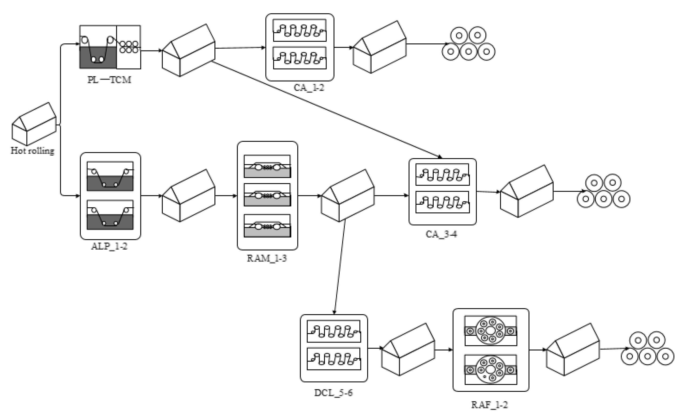
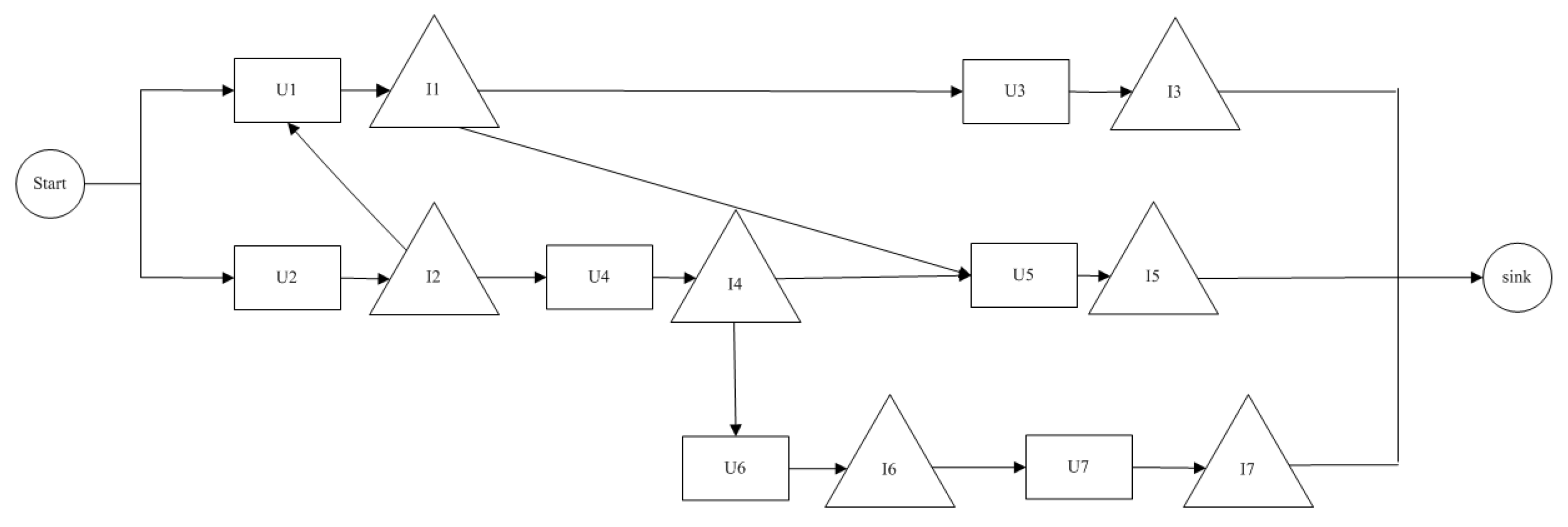
As the last stage of steel production, there are many different finished products in the cold rolling processes according to the customers’ demands. The topology network structure for cold rolling is shown in Figure 2, in which each square represents a processing unit, and each triangle represents an intermediate storage warehouse. For each processing unit in cold rolling production, there are multiple parallel machines. The source of cold rolling is the output products from the last hot rolling stage. At the start node, the production process starts with rolled coils from the hot rolling mill, which are assumed to be unlimited. When changing from one product type to another on a machine, the production changeover occurs. The intermediate buffer inventory is used to store the semi-finished products between the adjacent processing units. The final product inventory of the cold rolling processes is used to satisfy the demand for different steel products. There are three main challenging considerations for the real production and inventory planning, which are described as the following:

• Stochastic product yields. One main characteristic of cold rolling production is uncertain product yields, which are caused by production conditions with uncertainties such as material imperfections, capacity limitations, and process environmental factors such as temperature and humidity. There are both uncertain production and storage factors that cause stochastic product yields during the cold rolling production stage. For the cold rolling processes, the coils are stretched, leveled, welded, and cut, which are not perfect production processes. For example, the real production speeds of the cold rolling machines are not determined, which may result in a mismatch between the processing units, leading to unbalanced products. The inventory stage can also create uncertainties for the product yields. For the final inventory storage in the cold rolling stage, long-term storage will cause the steel coil to rust, which leads to reduced product yields. Based on the real production and management analysis, we reduce the complicated, uncertain product yields in the final inventory level of the cold rolling products in this paper.
• Product-switching cost. There are different specifications for the final products of the cold rolling processes, which in turn require the unit setup for different types of steel products. Product switching occurs when a machine switches from manufacturing one product type to another. There are mainly two ways to make the switch. For the first way, some transition coils and are added and processed between two product types, which may achieve a smooth changeover without changing the rollers. For the second way, the rollers in some machines are replaced so that the production condition is reset. A substantial switching cost is incurred for both methods. The switching cost is the expense for the transition coils in the first method, while it is the cost of replacing the new rollers in the second method. To control the switching cost, we would like to reduce the number of product changeovers. However, a product changeover cannot be completely avoided due to multi-product demand. Therefore, there is a trade-off between the product changeovers and the product inventory for the production planning of the cold rolling processes.
• Continuous Process and Inventory buffers. To increase the production capacity in the cold rolling stage, it is important to maintain the continuity of the production processes. Considering the different production speeds for the units, the intermediate buffer storage is used to support the downstream continuous process. The downstream production process is interrupted if there is an insufficient inventory quantity to feed the following process. There is also the capacity and cost for the intermediate buffer within the cold rolling processes. The coordinate of the inventory quantity and inventory cost is important for production and inventory planning to satisfy the market demand for the steel plant.

The production and inventory planning for the cold rolling processes with consideration of random yields aims to determine the production and inventory quantity of each final steel product in the machines and units for each period to satisfy a given set of product orders for multiple steel coils with different specifications within a finite planning horizon. The optimization objective is to minimize the total expected cost, which includes the switching cost of the products, inventory cost, production cost, and the backorder penalty. The real production constraints, such as the production capacity and inventory limitations, must be to satisfied. Here, we assume that uncertain yields only influence the final product inventory quantity.

3.2. Mathematical Formulation

The notations in the proposed mathematical model are listed as:

• j: the index of product.
• $\mathcal{J}$: the set of all products, $\forall j\in \mathcal{J}$.
• t: the index of time period.
• $\mathcal{T}$: the set of all time periods, $\forall t\in \mathcal{T}$.
• $u:$ the index of unit.
• $\mathcal{U}$: the set of all units, $\forall u\in \mathcal{U}$.
• m: the index of machine.
• $M_u$: the subset of machines at unit u; every unit includes many machines, $\forall m\in M_u$.
• k: the index of stage.
• $k_j$: the number of stages that product j goes through, $\forall k\in 1,2,\dots ,k_j$.
• $a(j,k)$: the index of unit that is the kth stage of product j.
• ${\rho }_{mj}$: the switching cost of product j on machine m.
• $h_{uj}$: the echelon-holding cost of product j on unit u.
• ${\varphi }_j$: the production cost of product j.
• $C_{mj}$: the capacity of machine m for product j.
• $r_j$: the order quantity of product j.
• $h_j^{T+1}$: the holding cost of inventory for product j in the last period.
• $b_j$: the backorder cost of inventory for product j in the last period.
• ${\underline{I}}_u$: the inventory lower limit for the intermediate buffer located after unit u.
• ${\overline{I}}_u$: the inventory upper limit for the intermediate buffer located after unit u.

The variables for the problem are defined as follows:

• $q_{mjt}$: decision variable representing the production quantity of product j on machine m at time period t.
• $I_{ujt}$: decision variable representing the inventory quantity of product j in the intermediate buffer located after unit u at time period t.
• $Y_{mjt}$: binary variable, whether to produce product j on machine m at time period t.
• $Z_{mjt}$: binary variable, whether to switch product j on machine m at time period t.
• ${\beta }_j$: random variable to represent the uncertain ratio of the inventory of the final steel product j.

With the above defined notions, a stochastic mathematical model for the production and inventory planning problem with uncertainties is formulated as follows:

$$\begin{array}{cc}\hfill \underset{q,I,Y,Z}{min}& \sum _{t\in \mathcal{T}}\sum _{u\in \mathcal{U}}\sum _{m\in M_u}\sum _{j\in \mathcal{J}}{\rho }_{mj}{Z}_{mjt}+\sum _{t\in \mathcal{T}}\sum _{u\in \mathcal{U}}\sum _{j\in \mathcal{J}}{h}_{uj}{I}_{ujt}+\sum _{t\in \mathcal{T}}\sum _{u\in \mathcal{U}}\sum _{m\in M_u}\sum _{j\in \mathcal{J}}{\varphi }_j{Y}_{mjt}\hfill \end{array}$$

$$\begin{array}{cc}\hfill & +E_{\beta }\left[\sum _{j\in \mathcal{J}}{h}_j^{T+1}{({\beta }_j{I}_{a(j,k_j),j,T}-r_j)}^{+}+\sum _{j\in \mathcal{J}}{b}_j{(r_j-{\beta }_j{I}_{a(j,k_j),j,T})}^{+}\right]\hfill \end{array}$$

(1)

$$\begin{array}{cc}\hfill \mathrm{s}.\mathrm{t}.& q_{mjt}\le C_{mj}{Y}_{mjt},\forall j\in \mathcal{J},u\in \mathcal{U},m\in M_u,t\in \mathcal{T},\hfill \\ \hfill & I_{a(j,k),j,t}=I_{a(j,k),j,t-1}\hfill \end{array}$$

(2)

$$\begin{array}{cc}\hfill & +\sum _{m\in M_{a(j,k)}}{q}_{mjt}-\sum _{m\in M_{a(j,k+1)}}{q}_{mjt},\forall j\in \mathcal{J},k=1,2,\dots ,k_j,t\in \mathcal{T},\hfill \end{array}$$

(3)

$$\begin{array}{cc}\hfill & {\underline{I}}_u\le \sum _{j\in \mathcal{J}}{I}_{ujt}\le {\overline{I}}_u,\forall u\in \mathcal{U},t\in \mathcal{T},\hfill \end{array}$$

(4)

$$\begin{array}{cc}\hfill & \sum _{j\in \mathcal{J}}{Y}_{mjt}\le 1,\forall u\in \mathcal{U},m\in M_u,t\in \mathcal{T},\hfill \end{array}$$

(5)

$$\begin{array}{cc}\hfill & Z_{mjt}\ge {(Y_{m,j,t}-Y_{m,j,t-1})}^{+},\forall j\in \mathcal{J},u\in \mathcal{U},m\in M_u,t\in \mathcal{T},\hfill \end{array}$$

(6)

$$\begin{array}{cc}\hfill & q_{mjt}\ge 0,I_{ujt}\ge 0,\forall m\in M_u,j\in \mathcal{J},u\in \mathcal{U},t\in \mathcal{T},\hfill \end{array}$$

(7)

$$\begin{array}{cc}\hfill & Z_{mjt},Y_{mjt}\in \{0,1\},\forall j\in \mathcal{J},u\in \mathcal{U},m\in M_u,t\in \mathcal{T}.\hfill \end{array}$$

(8)

The objective Function (1) aims to minimize the total expected cost, which includes the switching cost between the different products, inventory-holding cost for intermediate products, production cost, and expected inventory-holding cost for the final products or the backorder penalty. We use the final inventory quantity of product j times the random variables ${\beta }_j$ to represent the final uncertain inventory of product j. If the actual inventory quantity of product j is greater than the required quantity, there will be an inventory cost for product j. Otherwise, a backorder penalty for the final product is added. Constraint (2) is the processing capacity constraint for the machines in each processing unit. Product j can only be produced on machine m at time period t if machine m is set up to produce product j at time t, in which case the maximum production quantity of product j is constrained by the capacity of machine m. Constraint (3) is the inventory balance constraint for each time period t. The inventory quantity of product j in time period t is equal to the remaining inventory quantity in time period $t-1$ plus the production quantity from the upstream unit, and minus the consumption quantity of the downstream unit. The final products are stored in the warehouse and used to satisfy the demand. Constraint (4) enforces the lower and upper bounds for the inventory quantity following the processing unit u. The lower bound of the product inventory quantity can be set to 0 if there are no specific requirements for the inventory. It can also be set as the safety stock level to ensure the continuity of the production of subsequent units. The upper bound is used to prevent the inventory level from going up without limits. It can also be used to reflect the physical capacity of the warehouse. In fact, it is mainly the latter. The upper bound prevents unlimited increases, as this would have no practical justification. Constraint (5) represents that, at most, one product type is produced on each machine in each period. Constraint (6) detects product switches in period t by comparing the product produced in periods $t-1$ and t. Note that we implicitly assume that there is at most one product switch in each period. This is a reasonable assumption due to the high cost of product switches. We note that it is possible to incorporate product switches on a finer time scale by redefining the time periods. For example, instead of defining each period as a day, we can define each period as six hours. The inequalities (7) are nonnegativity constraints for the production quantity and inventory. The last Equation (8) enforces binary conditions on the switching and production variables.

The proposed mathematical formulation for production and inventory planning with uncertainty is a stochastic programming model that is nonlinear. Due to the random yield, the objective function involves an expectation that is bilinear and discontinuous. Therefore, there is no direct exact solution method for this proposed model. In the next section, we deduce the two lower bounds for the expected objective function, then develop the lower bounds-based heuristics for the problem with consideration of the stochastic yields.

4. Bounds and Heuristics

We first deduce two lower bounds for the objective function of the proposed stochastic model in Section 3. The first lower bound is based on relaxing the full information and is introduced in Section 4.1. The second lower bound is based on Jensen’s inequality and takes advantage of the objective function’s convexity. This bound is introduced in Section 4.2. Then, we develop heuristics based on the proposed lower bounds. Finally, we propose a two-step procedure based on the newsvendor model in Section 4.3.

4.1. Full Information Relaxation-Based Bound and Heuristic I

For a given realization of the random yield $\beta$, the production and inventory planning problem is a deterministic programming problem that can be solved using general purpose integer programming solvers. One way to address this computational challenge is to solve a series of deterministic program problems, where each is associated with a sampled value of the random yield $\beta$. That is, we first sample the random yield $\beta$ and then solve the problem for the sampled value of $\beta$. Instead of imposing expectations on the objective function in the proposed stochastic model, the average objective value for all sampled $\beta$ is taken to be an approximation of the optimal objective function, which is called the bound based on the full information. This method is well known in stochastic programming and was proposed by Prekapa [54] and is sometimes called full information relaxation because it assumes complete information of the random variable $\beta$. It is straightforward to show that full information relaxation is a lower bound of the primal stochastic objective function. We summarize the result in Proposition 1.

Proposition 1.

The full information relaxation leads to a lower bound of the objective value of the stochastic production and inventory planning problem.

Proof. 

Let $f(\beta ,q,I,Y,Z)$ denote the objective function of the stochastic production and inventory planning problem. The expectation of the objective value is given by $E_{\beta }\left[f(\beta ,q,I,Y,Z)\right]$. Instead of minimizing this expectation, full information relaxation aims to find the optimal objective values for each sample $\beta$ in the random field, then takes the average value of all obtained optimal objective values as an approximation of the primal optimal objective value.

Let $(q^{*},I^{*},Y^{*},Z^{*})$ denote the optimal solution of the stochastic production and inventory planning problem, and let $(q^{*}\left(\beta \right),I^{*}\left(\beta \right),Y^{*}\left(\beta \right),Z^{*}\left(\beta \right))$ denote the optimal solution for a given $\beta$. Because the primal problem involves minimization, we must have

$$E_{\beta }\left[f(\beta ,q^{*}\left(\beta \right),I^{*}\left(\beta \right),Y^{*}\left(\beta \right),Z^{*}\left(\beta \right))\right]\le E_{\beta }\left[f(\beta ,q^{*},I^{*},Y^{*},Z^{*})\right].$$

This completes the proof. □

Proposition 1 is a general result for the stochastic production and inventory planning problem. Based on Proposition 1, some approximation solution methods for the stochastic planning problem can be designed. Note that the optimization problem corresponding to each fixed $\beta$ is still a nonlinear optimization problem. However, we can rewrite it as a linear problem using reformulation techniques in integer programming.

It is not immediately clear how we can generate a heuristic policy for the production and inventory planning problem, given that there is a set of values for the decision variables corresponding to each $\beta$. Because some of the variables are required to be integer variables, averaging the solutions will create some fractional solutions that are not feasible. In this paper, we use the solution corresponding to the median of the sampled random yield to generate a heuristic policy, which is Heuristic I. The proper pseudo-code of Heuristic I is presented as the following:

Heuristic I:

Step 1. Generate the samples of production yield;

Step 2. Calculate the median of the sample set of production yield, ${\beta }^m$;

Step 3. Replace $\beta$ with ${\beta }^m$, then the objective Function (1) is reduced into

$$\begin{array}{cc}\hfill \underset{q,I,Y,Z}{min}& \sum _{t\in \mathcal{T}}\sum _{u\in \mathcal{U}}\sum _{m\in M_u}\sum _{j\in \mathcal{J}}{\rho }_{mj}{Z}_{mjt}+\sum _{t\in \mathcal{T}}\sum _{u\in \mathcal{U}}\sum _{j\in \mathcal{J}}{h}_{uj}{I}_{ujt}+\sum _{t\in \mathcal{T}}\sum _{u\in \mathcal{U}}\sum _{m\in M_u}\sum _{j\in \mathcal{J}}{\varphi }_j{Y}_{mjt}+\hfill \\ \hfill & \left[\sum _{j\in \mathcal{J}}{h}_j^{T+1}{({\beta }_j^m{I}_{a(j,k_j),j,T}-r_j)}^{+}\sum _{j\in \mathcal{J}}{b}_j{(r_j-{\beta }_j^m{I}_{a(j,k_j),j,T})}^{+}\right]\hfill \end{array}$$

(9)

Step 4. Solve the reduced model with CPLEX solver. The optimal solution of the reduced model is the optimal control policy of Heuristic I.

4.2. Jensen’s Inequality-Based Bound and Heuristic II

If we replace the random yield $\beta$ with the mean value of $\beta$, the stochastic objective Function (5) has a certain good structure. Therefore, we introduce a new lower bound based on Jensen’s inequality and proved by Jensens [55]. To apply Jensen’s inequality, we first show that the function $f(\beta ,q,I,Y,Z)$ is convex for a given $\beta$.

Lemma 1.

The objective function $f(\beta ,q,I,Y,Z)$ is convex for a given β.

Proof. 

Note that the random variable $\beta$ only appears in the last two terms in the objective function $f(\beta ,q,I,Y,Z)$. For each $j\in \mathcal{J}$, the terms $h_j^{T+1}{({\beta }_j{I}_{a(j,k_j),j,T}-r_j)}^{+}$ and $b_j{(r_j-{\beta }_j{I}_{a(j,k_j),j,T})}^{+}$ are both convex for a given $\beta$. The objective function is convex because the sum of the convex functions are convex. This completes the proof. □

Based on Lemma 1, we use the expectation of the random variable $\beta$ to replace the random variables. Then, the objective function $E_{\beta }\left[f(\beta ,q,I,Y,Z)\right]$ is transformed into $f\left(E\right[\beta ],q,I,Y,Z)$. Due to the convexity of $f(\beta ,q,I,Y,Z)$ for a given $\beta$, we have

$$E_{\beta }\left[f(\beta ,q,I,Y,Z)\right]\ge f(E\left[\beta \right],q,I,Y,Z).$$

This immediately implies that replacing the primal objective function $E_{\beta }\left[f(\beta ,q,I,Y,Z)\right]$ with $f\left(E\right[\beta ],q,I,Y,Z)$ produces a lower bound of the primal objective optimum.

Proposition 2.

Replacing the objective function $E_{\beta }\left[f(\beta ,q,I,Y,Z)\right]$ with $f\left(E\right[\beta ],q,I,Y,Z)$ produces a lower bound to the stochastic production and inventory planning problem.

The bound in Proposition 2 is called the lower bound based on Jensen’s inequality. To obtain the lower bound, we only need to solve the stochastic production and inventory planning problem, assuming the given mean random yield. The solution method for lower bound II immediately implies a heuristic control policy. Heuristic II is based on lower bound II, and the procedure is given in the following:

Heuristic II:

Step 1. Set the mean of the production yield, ${\beta }^{mn}$;

Step 2. The objective Function (1) is replaced with

$$\begin{array}{cc}\hfill \underset{q,I,Y,Z}{min}& \sum _{t\in \mathcal{T}}\sum _{u\in \mathcal{U}}\sum _{m\in M_u}\sum _{j\in \mathcal{J}}{\rho }_{mj}{Z}_{mjt}+\sum _{t\in \mathcal{T}}\sum _{u\in \mathcal{U}}\sum _{j\in \mathcal{J}}{h}_{uj}{I}_{ujt}+\sum _{t\in \mathcal{T}}\sum _{u\in \mathcal{U}}\sum _{m\in M_u}\sum _{j\in \mathcal{J}}{\varphi }_j{Y}_{mjt}\hfill \\ \hfill & +\left[\sum _{j\in \mathcal{J}}{h}_j^{T+1}{({\beta }_j^{mn}{I}_{a(j,k_j),j,T}-r_j)}^{+}+\sum _{j\in \mathcal{J}}{b}_j{(r_j-{\beta }_j^{mn}{I}_{a(j,k_j),j,T})}^{+}\right]\hfill \end{array}$$

(10)

Step 3. Generate the deterministic MIP model with the mean of production yields.

Step 4. Solve the generated MIP model with CPLEX solver, then obtain the optimal control policy.

4.3. Newsvendor Logic-Based Heuristic III

Section 4.1 and Section 4.2 introduce two lower bounds and two corresponding heuristics for the stochastic production and inventory planning problem. This section introduces a heuristic based on the newsvendor model. The newsvendor (or newsboy) model proposed by Stevenson [56] is a mathematical model used in operations management and applied economics to determine optimal inventory levels.

Observing that the major complication in the stochastic production and inventory planning problem comes from the expectation term in the objective function, we propose a two-stage procedure to solve the problem. In the first stage, we find the inventory level that minimizes the expectation inventory-holding and backorder costs by ignoring the constraints. That is, we solve the problem:

$$\begin{array}{cc}\hfill & \underset{I_{a(j,k_j),j,T}\forall j\in \mathcal{J}}{min}{E}_{\beta }\left[\sum _{j\in \mathcal{J}}{h}_j^{T+1}{({\beta }_j{I}_{a(j,k_j),j,T}-r_j)}^{+}+\sum _{j\in \mathcal{J}}{b}_j{(r_j-{\beta }_j{I}_{a(j,k_j),j,T})}^{+}\right]\hfill \\ \hfill & =\sum _{j\in \mathcal{J}}\underset{I_{a(j,k_j),j,T}}{min}{E}_{\beta }\left[h_j^{T+1}{({\beta }_j{I}_{a(j,k_j),j,T}-r_j)}^{+}+b_j{(r_j-{\beta }_j{I}_{a(j,k_j),j,T})}^{+}\right].\hfill \end{array}$$

(11)

As shown above, the optimization problem is naturally decomposable by product j. Therefore, we can respectively solve the problem for each product. The structure of the optimization problem is reduced to the newsvendor problem. For each $j\in \mathcal{J}$, let

$$\begin{array}{c}\hfill c({\beta }_j,I_j)=E_{\beta }[h_j^{T+1}{({\beta }_j{I}_j-r_j)}^{+}+b_j{(r_j-{\beta }_j{I}_j)}^{+}].\end{array}$$

(12)

Lemma 2.

The function $c({\beta }_j,I_j)$ is convex in $I_j$ for each product j, and there exists an optimal inventory $I_j^{*}$ that satisfies the first-order condition $h_j^{T+1}E\left[{\beta }_j\right]-(h_j^{T+1}+b_j){\int }_0^{\frac{r_j}{I_j}}{\beta }_{j}dF\left({\beta }_j\right)=0$.

Proof. 

For each product $j\in \mathcal{J}$, the function $c({\beta }_j,I_j)=E_{\beta }[h_j^{T+1}{(\beta I_j-r_j)}^{+}+b_j{(r_j-\beta I_j)}^{+}]$ is convex in $I_j$. We have

$$\begin{array}{cc}\hfill c(\beta ,I)& =E_{\beta }(h{(\beta I-r)}^{+}+b{(r-\beta I)}^{+})\hfill \\ \hfill & ={\int }_0^{\frac{r}{I}}b(r-xI)dF\left(x\right)+{\int }_{\frac{r}{I}}^{1}h(xI-r)dF\left(x\right).\hfill \end{array}$$

(13)

In the above, $F(·)$ is the cumulative distribution function of the random variable $\beta$, $f(·)$ is the probability density function of the random variable $\beta$, and $\beta \in (0,1]$. The first-order derivative is

$$\begin{array}{cc}\hfill \frac{\partial c(\beta ,I)}{\partial I}& =-b{\int }_0^{\frac{r}{I}}xdF\left(x\right)+b(\frac{r}{I}I-r)f\left(\frac{r}{I}\right)\frac{\partial \left(\frac{r}{I}\right)}{\partial I}+h{\int }_{\frac{r}{I}}^{1}xdF\left(x\right)-h(r-\frac{r}{I}I)f\left(\frac{r}{I}\right)\frac{\partial \left(\frac{r}{I}\right)}{\partial I}\hfill \\ \hfill & =-b{\int }_0^{\frac{r}{I}}xdF\left(x\right)+h{\int }_{\frac{r}{I}}^{1}xdF\left(x\right)\hfill \\ \hfill & =-b{\int }_0^{\frac{r}{I}}xdF\left(x\right)+h[{\int }_0^{1}xdF\left(x\right)-{\int }_0^{\frac{r}{I}}xdF\left(x\right)]\hfill \\ \hfill & =-b{\int }_0^{\frac{r}{I}}xdF\left(x\right)+h[E\left(x\right)-{\int }_0^{\frac{r}{I}}xdF\left(x\right)]\hfill \\ \hfill & =hE\left[x\right]-(h+b){\int }_0^{\frac{r}{I}}xdF\left(x\right).\hfill \end{array}$$

(14)

The second-order derivative is

$$\begin{array}{cc}\hfill \frac{{\partial }^{2}c(\beta ,I)}{\partial I^2}& =-(h+b)\frac{r}{I}f\left(\frac{r}{I}\right)(-\frac{r}{I^2})\hfill \\ \hfill & =(h+b)\frac{r^2}{I^3}f\left(\frac{r}{I}\right)\ge 0\hfill \end{array}$$

(15)

It follows that $c(\beta ,I)$ is convex in I. Hence, the first-order condition is both necessary and sufficient. This completes the proof. □

For each product j, let ${\tilde{I}}_{a(j,k_j),j,T}$ be the optimal solution for (11) for the j-th subproblem. In the second stage, we replace the demand quantity $r_j$ with ${\tilde{I}}_{a(j,k_j),j,T}$ for each product j. That is, we replace the expectation term in the objective function of the stochastic production and inventory planning problem with

$$\begin{array}{c}\hfill \sum _{j\in \mathcal{J}}{h}_j^{T+1}{(I_{a(j,k_j),j,T}-{\tilde{I}}_{a(j,k_j),j,T})}^{+}+\sum _{j\in \mathcal{J}}{b}_j{({\tilde{I}}_{a(j,k_j),j,T}-I_{a(j,k_j),j,T})}^{+}.\end{array}$$

(16)

Instead of considering the random variable ${\beta }_j$, we order an inflated amount ${\tilde{I}}_{a(j,k_j),j,T}$ for each product. Therefore, the resulting problem is transformed into a deterministic optimization problem that can be solved through a general solver.

The proposed two-stage procedure can be directly used as Heuristic III for the stochastic production and inventory planning problem. For Equation (11), the optimal inventory $F\left(I^{*}\right)=\frac{r(h+b)}{hE\left(\beta \right)}$ is related to the demand order quantity, the mean value of the random variable, and the holding cost for the final product and backorder cost. In particular, the optimal production quantity for each product is linearly increasing in the demand order quantity. The newsvendor logic-based heuristic for the production and inventory planning problem is given as the following:

Heuristic III:

Stage 1.

Step 1-1. Construct the newsvendor problem for each product, as Equation (12);

Step 1-2. Solve all the newsvendor problems, then obtain the optimal inventory quantity, ${\tilde{I}}_{a(j,k_j),j,T}$;

Stage 2.

Step 2-1. Replace the demand quantity $r_j$ with ${\tilde{I}}_{a(j,k_j),j,T}$ for each product j, then the stochastic terms in Equation (1) are changed into Equation (16);

Step 2-2. The primal model is reduced into a deterministic MIP model, which can be solved with CPLEX solver;

Step 2-3. The optimal solution of the reduced MIP model is an optimal control policy.

5. Numerical Results

In this paper, we evaluated the proposed bounds and heuristics through computational experiments on a number of problem instances. These problem instances were generated randomly based on real information from a cold rolling plant in China. Two models for calculating the lower bound and three heuristics were implemented in the Python programming language, and a commercial CPLEX solver was used for the mixed integer programs. The computation time for each mixed integer program is limited to 1 h for an instance to prevent prolonged execution time. All tests were operated on a personal computer with Intel 2.5 GHz and 8 GB RAM.

The remainder of this section is organized as follows. Section 5.1 introduces how to generate the test instances and experimental setup. Section 5.2 reports the numerical experimental results of the bounds and heuristics. Section 5.3 conducts a sensitivity analysis.

5.1. Test Instances and Experimental Setup

Based on an analysis of the actual production environment of the cold rolling plant, we generate a set of random problem instances to evaluate the performance of the proposed bounds and heuristics. Each problem instance can be specified by the configuration of the production network, distribution of the random yield, and cost parameters. The configuration of the production network is denoted by a triplet $(U,M,J)$, where U is the number of units, M is the number of machines in each unit, and J is the number of products to be produced. Each product is associated with a distinguished path in the production network. Although there are many combinations of paths in the production network, we only choose the one that is consistent with the actual production situation for each product. One level of the number of units (U = 3), and one level of the number of machines for each unit (M = 3), and four levels of the number of products (U = 3, 4, 5, and 6) were considered. Based on the actual plan implementation, the length of the planning horizon T is set as 7.

The capacity for each machine is set at 100. The mean value of the order quantity is set at 150 for each product. To coincide with the actual production, the random yield is assumed to follow the beta distribution. For the beta distribution of the yield, two levels of the expected values ($\mu$ = 0.75 and 0.9) and four levels of the variance (${\sigma }^2$ = ${0.1}^2$, ${0.2}^2$, ${0.3}^2$, ${0.4}^2$ if $\mu$ = 0.75; and ${\sigma }^2$ = ${0.1}^2$, ${0.15}^2$, ${0.2}^2$, ${0.25}^2$ if $\mu$ = 0.9) were considered.

The product switching cost is assumed to be larger than the backorder cost, which is set at 3 to 5 times that of the steel price. The holding cost is considered lower than the backorder cost. The holding cost from the intermediate product is computed by multiplying the interest rate per period by the price of the steel products.

5.2. Performance of Bounds and Heuristics

Table 1. Numerical results for two bounds and three heuristics with E($\beta$) = 0.75. The holding costs for the intermediate product and the final product are 5 and 100, respectively.

$(\mathit{\mu },{\mathit{\sigma }}^2)$	$(\mathit{U},\mathit{M},\mathit{J})$	${\mathit{LB}}_1$	${\mathit{LB}}_2$	${\mathit{OBJ}}_1$	${\mathit{Gap}}_1$(%)	${\mathit{OBJ}}_2$	${\mathit{Gap}}_2$(%)	${\mathit{OBJ}}_3$	${\mathit{Gap}}_3$(%)
$(0.75,{0.1}^2)$	(3, 3, 3)	54,825	46,500	58,685	6.6	57,964	5.4	58,040	5.5
	(3, 3, 4)	108,896	98,000	109,214	0.3	108,964	0.1	108,964	0.1
	(3, 3, 5)	117,730	105,500	120,285	2.1	120,285	2.1	119,884	1.8
	(3, 3, 6)	125,933	113,000	132,971	5.3	131,606	4.3	131,804	4.5
$(0.75,{0.2}^2)$	(3, 3, 3)	65,222	46,500	75,576	13.7	72,949	10.6	73,520	11.3
	(3, 3, 4)	116,407	98,000	125,462	7.2	123,949	6.1	123,949	6.1
	(3, 3, 5)	126,262	105,500	144,353	12.5	140,265	10.0	140,143	9.9
	(3, 3, 6)	136,060	113,000	161,127	15.6	156,582	13.1	157,337	13.5
$(0.75,{0.3}^2)$	(3, 3, 3)	77,239	46,499	91,536	15.6	88,676	12.9	89,431	13.6
	(3, 3, 4)	128,147	97,999	142,204	9.9	139,702	8.3	139,680	8.3
	(3, 3, 5)	136,611	105,499	164,430	16.9	161,192	15.2	161,783	15.6
	(3, 3, 6)	157,718	112,999	186,038	15.2	182,817	13.7	184,890	14.7
$(0.75,{0.4}^2)$	(3, 3, 3)	83,700	46,500	97,498	14.2	105,280	20.5	97,498	14.2
	(3, 3, 4)	132,997	98,000	147,747	10.0	156,280	14.9	147,775	10.0
	(3, 3, 5)	149,718	105,500	172,997	13.5	183,373	18.4	172,997	13.5
	(3, 3, 6)	173,577	113,000	197,991	12.3	210,467	17.5	197,978	12.3

,

Table 2. Numerical results for two bounds and three heuristics with E($\beta$) = 0.9. The holding costs for the intermediate product and the final product are 5 and 100, respectively.

$(\mathit{\mu },{\mathit{\sigma }}^2)$	$(\mathit{U},\mathit{M},\mathit{J})$	${\mathit{LB}}_1$	${\mathit{LB}}_2$	${\mathit{OBJ}}_1$	${\mathit{Gap}}_1$(%)	${\mathit{OBJ}}_2$	${\mathit{Gap}}_2$(%)	${\mathit{OBJ}}_3$	${\mathit{Gap}}_3$(%)
$(0.9,{0.1}^2)$	(3, 3, 3)	46,549	44,500	55,568	16.2	53,472	12.9	52,530	11.4
	(3, 3, 4)	88,487	88,000	99,604	11.2	96,472	8.3	95,729	7.6
	(3, 3, 5)	97,673	95,333	108,642	10.1	106,796	8.5	105,540	7.5
	(3, 3, 6)	104,419	102,500	119,627	12.7	116,953	10.7	115,251	9.4
$(0.9,{0.15}^2)$	(3, 3, 3)	51,381	44,500	60,124	14.5	58,320	11.9	58,196	11.7
	(3, 3, 4)	95,606	88,000	103,627	7.7	101,320	5.6	101,356	5.7
	(3, 3, 5)	102,618	95,333	116,919	12.2	113,261	9.4	113,125	9.3
	(3, 3, 6)	107,493	102,500	129,193	16.8	125,034	14.0	124,720	13.8
$(0.9,{0.2}^2)$	(3, 3, 3)	58,130	44,500	63,193	8.0	62,422	6.9	62,349	6.8
	(3, 3, 4)	97,043	88,000	106,341	8.7	105,422	7.9	105,327	7.9
	(3, 3, 5)	10,6344	95,333	120,250	11.6	118,729	10.4	118,703	10.4
	(3, 3, 6)	11,4752	102,500	133,928	14.3	131,870	13.0	131,762	12.9
$(0.9,{0.25}^2)$	(3, 3, 3)	56,069	44,500	63,749	12.0	65,920	14.9	91,185	38.5
	(3, 3, 4)	96,044	88,000	106,499	9.8	108,920	11.8	118,094	18.7
	(3, 3, 5)	102,814	95,333	120,499	14.7	123,394	16.7	136,870	24.9
	(3, 3, 6)	125,489	102,500	129,515	3.1	137,700	8.9	155,169	19.1

,

Table 3. Numerical results for two bounds and three heuristics with E($\beta$) = 0.75. The holding costs for the intermediate product and the final product are 1 and 30, respectively.

$(\mathit{\mu },{\mathit{\sigma }}^2)$	$(\mathit{U},\mathit{M},\mathit{J})$	${\mathit{LB}}_1$	${\mathit{LB}}_2$	${\mathit{OBJ}}_1$	${\mathit{Gap}}_1$(%)	${\mathit{OBJ}}_2$	${\mathit{Gap}}_2$(%)	${\mathit{OBJ}}_3$	${\mathit{Gap}}_3$(%)
$(0.75,{0.1}^2)$	(3, 3, 3)	47,224	38,100	50,944	7.3	50,276	6.1	48,542	2.7
	(3, 3, 4)	97,979	86,800	100,865	2.9	98,876	0.9	98,876	0.9
	(3, 3, 5)	106,436	93,100	109,519	2.8	109,235	2.6	107,298	0.8
	(3, 3, 6)	111,156	99,399	121,151	8.2	119,594	7.1	115,920	4.1
$(0.75,{0.2}^2)$	(3, 3, 3)	55,050	38,100	66,739	17.5	63,513	13.3	85,637	35.7
	(3, 3, 4)	106,940	86,800	116,318	8.1	112,113	4.6	155,137	31.1
	(3, 3, 5)	116,278	93,100	132,124	12	126,884	8.4	167,471	30.6
	(3, 3, 6)	123,950	99,399	146,677	15.5	141,655	12.5	179,905	31.1
$(0.75,{0.3}^2)$	(3, 3, 3)	66,343	38,099	85,655	22.5	77,406	14.3	97,550	32
	(3, 3, 4)	113,815	86,799	132,898	14.4	126,031	9.7	167,050	31.9
	(3, 3, 5)	124,291	93,099	155,602	20.1	145,433	14.5	163,464	24
	(3, 3, 6)	139,306	99,399	179,853	22.5	164,835	15.5	203,721	31.6
$(0.75,{0.4}^2)$	(3, 3, 3)	80,108	38,100	93,296	14.1	92,072	13	91,977	12.9
	(3, 3, 4)	123,400	86,800	141,747	12.9	140,672	12.3	140,554	12.2
	(3, 3, 5)	148,084	93,100	166,592	11.1	164,963	10.2	160,082	7.5
	(3, 3, 6)	158,029	99,399	191,393	17.4	189,254	16.5	189,111	16.4

and

Table 4. Numerical results for two bounds and three heuristics with E($\beta$) = 0.9. The holding costs for the intermediate product and the final product are 1 and 30, respectively.

$(\mathit{\mu },{\mathit{\sigma }}^2)$	$(\mathit{U},\mathit{M},\mathit{J})$	${\mathit{LB}}_1$	${\mathit{LB}}_2$	${\mathit{OBJ}}_1$	${\mathit{Gap}}_1$(%)	${\mathit{OBJ}}_2$	${\mathit{Gap}}_2$(%)	${\mathit{OBJ}}_3$	${\mathit{Gap}}_3$(%)
$(0.9,{0.1}^2)$	(3, 3, 3)	39,086	37,700	49,622	21.2	47,333	17.4	43,233	9.6
	(3, 3, 4)	81,265	78,799	90,026	9.7	88,333	8.0	83,819	3.0
	(3, 3, 5)	86,058	85,066	99,425	13.4	97,811	12.0	92,158	6.6
	(3, 3, 6)	95,116	91,299	110,220	13.7	107,256	11.3	100,698	5.5
$(0.9,{0.15}^2)$	(3, 3, 3)	41,226	37,700	56,322	26.8	51,616	20.1	48,077	14.3
	(3, 3, 4)	84,076	78,799	97,137	13.4	92,616	9.2	88,693	5.2
	(3, 3, 5)	92,398	85,066	109,702	15.8	103,522	10.7	98,564	6.3
	(3, 3, 6)	100,158	91,299	120,184	16.7	114,394	12.4	108,636	7.8
$(0.9,{0.2}^2)$	(3, 3, 3)	50,351	37,700	59,238	15.0	55,239	8.8	53,650	6.1
	(3, 3, 4)	89,735	78,799	100,198	10.4	96,239	6.8	94,215	4.8
	(3, 3, 5)	95,832	85,066	113,781	15.8	108,352	11.6	105,985	9.6
	(3, 3, 6)	104,316	91,299	126,695	17.7	120,432	13.4	117,955	11.6
$(0.9,{0.25}^2)$	(3, 3, 3)	51,654	37,700	59,547	13.3	58,329	11.4	58,265	11.3
	(3, 3, 4)	96,639	78,799	100,499	3.8	99,329	2.7	99,309	2.7
	(3, 3, 5)	98,258	85,066	114,099	13.9	112,473	12.6	112,387	12.6
	(3, 3, 6)	111,861	91,299	127,649	12.4	125,583	10.9	125,446	10.8

report the results of the above bounds and heuristics for the setting of different instances. In this experiment, the product switching cost is $\rho =5000$ and the backorder cost is $b=500$. The holding cost is shown in the tables. In total, there are two lower bounds and three heuristics. $OB{J}_1$, $OB{J}_2$, and $OB{J}_3$ correspond to the full information relaxation, Jensen’s inequality, and the newsvendor logic, respectively. $L{B}_1$ and $L{B}_2$ are the lower bounds based on the full information relaxation and Jensen’s inequality, respectively. The performance of the proposed heuristics can be benchmarked against the best lower bound. In particular, the performance gap $Ga{p}_i$ of heuristic i is computed as the relative error between the objective value and the best lower bound.

Overall, the bounds based on full information relaxation ($L{B}_1$) are better (larger) than the bounds based on Jensen’s inequality. However, the heuristics based on Jensen’s inequality and newsvendor logic perform better than the heuristic from full information relaxation. That may be because the feasible solution achieved by the full information relaxation method is obtained by solving the scenario with the median of the sampled random yield. The method can find an integral solution quickly. However, the quality of the solution is not competitive with the ones achieved by Jensen’s inequality and newsvendor logic.

The evaluated cost increases with the variance of the random yield for the same mean value. For constant variance, the total cost decreases in the mean value of the random yield. Comparing Table 1 and Table 2 (and Table 3 and Table 4), the relative performance of the heuristic based on Jensen’s inequality is better when E($\beta$) = 0.75. Comparing Table 1 and Table 3 (and Table 2 and Table 4), the heuristic based on newsvendor logic performs better as the backorder cost and holding cost decrease. Therefore, the performance of the proposed heuristics critically depends on the cost parameters and the random yield. Overall, changing the mean value of the random yield has a substantial impact on the performance of the three heuristics.

5.3. Sensitivity Analysis

In this section, we investigate the effect of changing model parameters on the performance of the three proposed heuristics. The model parameters include the process parameters (i.e., random yield) and cost parameters (i.e., switching, holding and backorder costs). We first consider the process parameters and then analyze the impact of the cost parameters. As the newsvendor heuristic performed the best in the previous numerical study, we conduct the sensitivity analysis by using this heuristic.

To analyze the impact of the mean and variance of the random variable distribution on the total cost, we consider the combinations of two mean values and four variances. The machine configuration is (3, 3, 3). The switching cost is $\rho =5000$. The holding costs for the intermediate and final product are $h=1$ and $h^{T+1}=100$. The backorder cost is $b=500$.

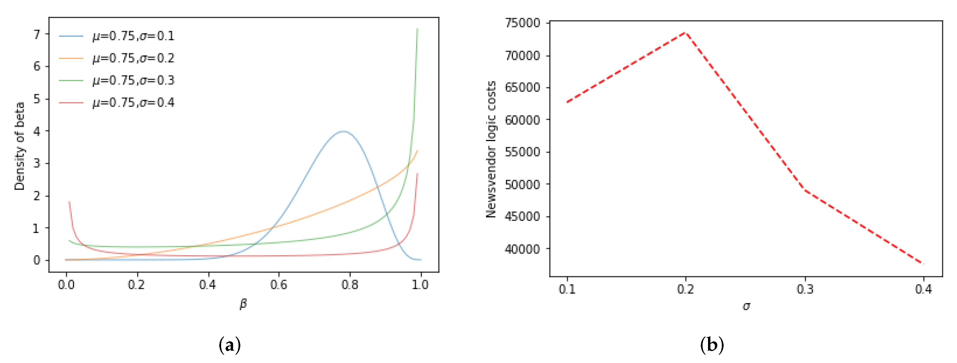
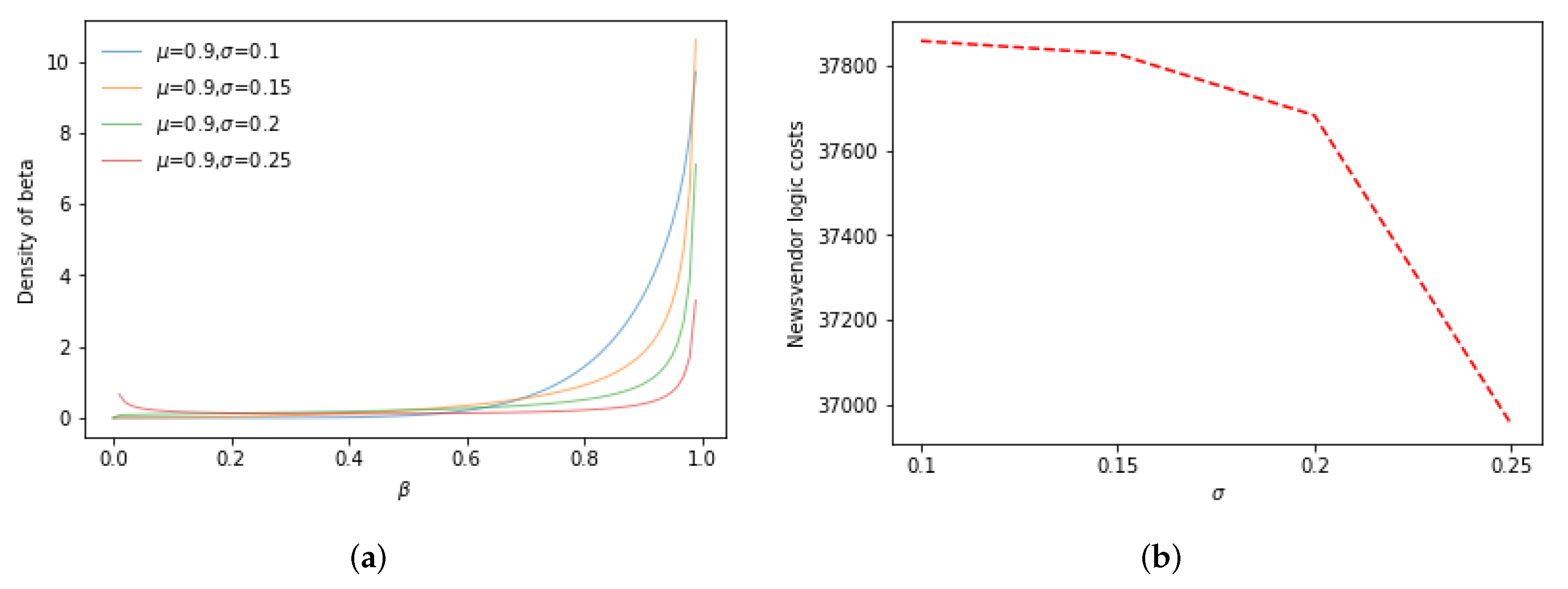
Figure 3a and Figure 4a show beta distributions with mean values of $0.75$ and $0.9$ denoted as $\mu$ and four different standard deviations denoted as $\sigma$. Figure 3b and Figure 4b show the corresponding costs from the newsvendor heuristic. Observe that the costs change dramatically and nonmonotonically as the variance increases. While the variance increases, the yield of each product is varied. However, the relevant objective function is related to the yield, but has no direct relationship with the variance of the yield distribution. Therefore, the objective function value changes as the distribution changes corresponding the change in variance, but it has no monotonic relationship with the change in variance.

Table 5. Numerical results for two bounds and three heuristics with different E($\beta$) when the variance is fixed at ${\sigma }^2={0.1}^2$.

$(\mathit{U},\mathit{M},\mathit{J})$	$\mathit{E}\left(\mathit{\beta }\right)$	${\mathit{LB}}_1$	${\mathit{LB}}_2$	${\mathit{OBJ}}_1$	${\mathit{OBJ}}_2$	${\mathit{OBJ}}_3$
$(3,3,6)$	0.90	104,041	102,500	120,210	116,953	115,251
	0.91	105,433	101,835	119,062	115,835	114,459
	0.92	103,378	101,173	118,593	114,625	113,610
	0.93	101,152	100,065	114,488	111,109	110,508
	0.94	101,782	99,861	115,042	111,737	111,481
	0.95	98,673	99,210	112,733	109,917	109,929
	0.96	101,006	98,562	108,713	107,679	107,692
	0.97	99,867	97,917	104,499	104,863	104,398

shows how the mean value of the random yield affects the cost when the machine configuration is given and the variance is fixed at ${0.1}^2$. A mean random yield from 0.90 to 0.97 is typical in practice. The switching cost is $\rho =5000$. The backorder cost is $b=500$. The holding costs for the intermediate and final products are $h=5$ and $h^{T+1}=100$. A higher mean value implies that the output of the unit is higher. Not surprisingly, the cost decreases as $E\left(\beta \right)$ increases. Hence, increasing the mean random yield is conducive to cost reduction. As the mean value increases, the yield increases, thus the inventory increases compared with the final product. Then, the production and inventory planning can be decided with less consideration of the product requirement, consequently reducing the related costs.

The inventory holding cost and backorder cost in the cold rolling plant are usually quite significant. The holding cost is mainly the capital cost tied up by the inventory. If there is no holding cost, each machine of the unit will produce as early as possible and as much as possible. Usually, the holding cost increases nearly linearly in product prices because the holding cost is often assumed to be a percentage of the product value. The suggested percentage ranges from 12% to 34% according to Berling [57]. The backorder cost mainly refers to the loss caused by the untimely delivery of orders. It is also quite natural to assume a higher backorder cost for a higher valued product.

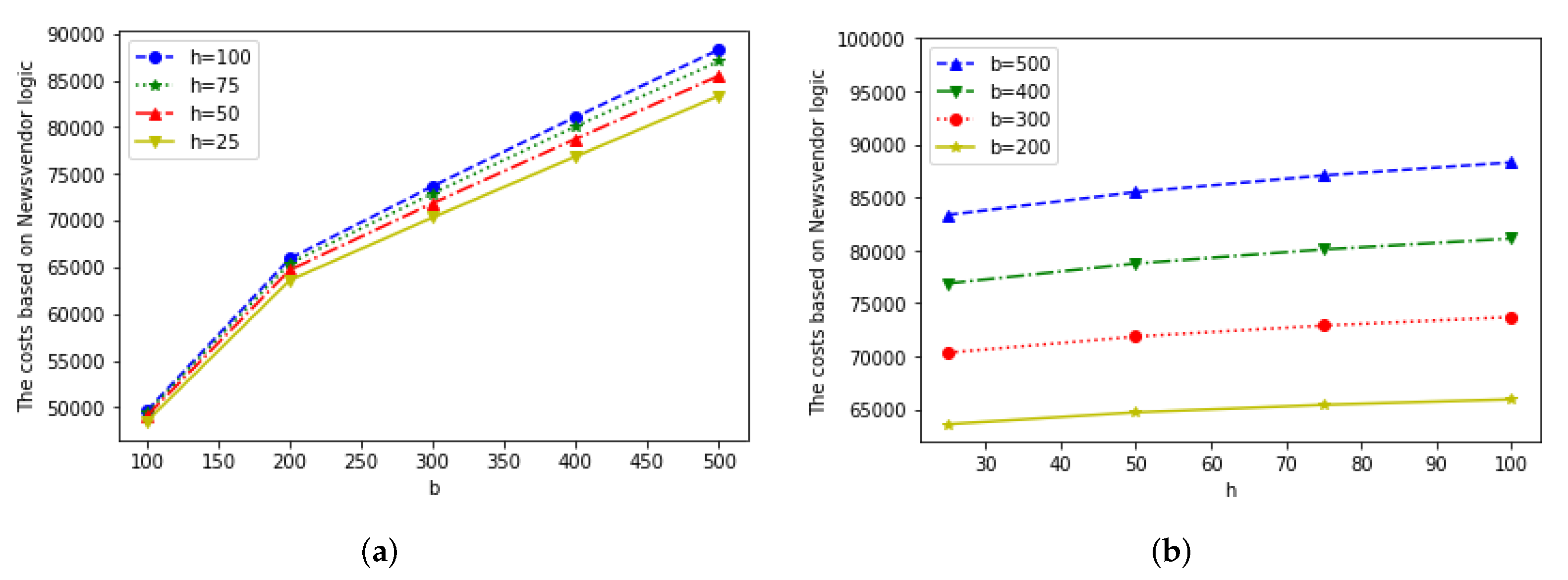
The total cost increases nearly linearly in the holding cost for the intermediate product and the switching cost. In fact, the switching cost appears to have a bigger impact than the holding cost for the intermediate product. Furthermore, having a substantial amount of excess inventory in the last period after all orders are fulfilled is very costly. Therefore, we mainly discuss the impact of the holding cost and the backorder cost in the last period. The product switching is $\rho =5000$. For $h^{T+1}=25,50,75$, and 100, we investigate the impact of the backorder cost b, which varies from 100 to 500. The results are shown in Figure 5a. For a given backorder cost, the total cost increases in the holding cost in the last period, given that the lines move up as the holding cost increases. This is further illustrated in Figure 5b. The backorder cost has a substantial impact on the total cost because the cost increases steeply as b increases in Figure 5a. One implication of this observation is that one must be careful in deciding the amount of orders to accept. Accepting more orders than the mill can produce can be very costly. We also implicate here that the inventory holding cost affects the switching times in production, even though it is not shown in Figure 5.

Table 6. Numerical results with different machine configurations.

$(\mathit{\mu },{\mathit{\sigma }}^2)$	$(\mathit{U},\mathit{M},\mathit{J})$	${\mathit{LB}}_1$	${\mathit{LB}}_2$	${\mathit{OBJ}}_1$	${\mathit{OBJ}}_2$	${\mathit{OBJ}}_3$
$(0.9,{0.1}^2)$	(6, 6, 3)	57,439	55,699	68,760	65,716	62,409
	(6, 7, 3)	54,991	55,033	70,375	65,049	61,638
	(6, 8, 3)	55,956	55,033	66,421	65,049	61,352
	(6, 9, 3)	55,533	55,033	62,169	65,116	61,738
	(6, 6, 4)	63,469	61,933	79,243	75,288	70,827
	(6, 7, 4)	61,909	61,600	82,033	74,854	70,441
	(6, 8, 4)	62,137	61,599	73,588	74,721	70,441
	(6, 9, 4)	63,334	61,266	72,724	74,688	70,148
	(6, 6, 5)	98,721	97,033	114,544	116,288	105,905
	(6, 7, 5)	62,041	74,499	95,471	90,960	85,630
	(6, 8, 5)	75,871	74,500	97,602	91,127	85,530
	(6, 9, 5)	80,844	74,166	91,737	90,927	85,337
	(6, 6, 6)	176,289	178,033	190,619	191,288	180,905
	(6, 7, 6)	121,834	121,600	146,850	138,193	132,708
	(6, 8, 6)	122,799	121,600	138,613	137,960	132,130
	(6, 9, 6)	118,983	121,300	153,635	137,860	131,744

shows the results for the different machine configurations. The total order quantity for each product is fixed at $r_j=150$. The switching cost is $\rho =5000$, the backorder cost is $b=500$, and the holding costs for the intermediate and final products are $h=1$ and $h^{T+1}=50$, respectively. The number of machines varies from 6 to 9. The number of products is from 3 to 6. In general, changing the machine configurations does not have a large impact on the total cost with the exception of a few instances (such as when $(U,M,J)=(6,6,5)$ and $(U,M,J)=(6,6,6)$). There appears to be a critical level of machine capacity below which the cost can blow up. Therefore, it is important to maintain sufficient machine capacity in the system. Even though our model does not explicitly consider decisions of order acceptance, our observation here implies that accepting too many orders can substantially increase the total cost if the required machine capacity is beyond a critical threshold. This can be observed when $(U,M,J)$ takes the values $(6,6,3)$ to $(6,6,6)$. Producing a large number of cold rolling products requires more frequent switches and higher inventory. Based on the results of the numerical experiments, we find that the number of products must be maintained within a certain range. Introducing a new product or machine can sometimes dramatically increase the costs. Therefore, one should carefully evaluate the situation before introducing the changes to the production process. Even though we do not consider the optimal design of the production paths, our model can be used to evaluate the impact of altering the production network or introducing new products.

6. Conclusions

This paper studies a production and inventory planning problem derived from cold rolling production. The problem is characterized by considering multi-stage production networks, multiple products distinguished by a production path, and a random yield. To address the problem, we formulate it as a nonlinear stochastic model with a nonlinear objective function. To solve the problem, full information relaxation and Jensen’s inequality-based lower bounds are proposed. Two simple heuristics are developed based on the proposed lower bounds. In addition, the third heuristic motivated by newsvendor logic is also proposed. Finally, the results of the numerical experiments based on real production data show the validity of the formulated model, the effectiveness of the proposed lower bounds, and the three heuristics. The sensitivity analysis for the solution method is also given, and the implications based on the numerical results are presented. In future work, we will consider the production and inventory planning problem under stochastic machine conditions, such as breakdowns and flexible processing rates.

References

- Karakostas, P.; Sifaleras, A.; Georgiadis, M.C. Adaptive variable neighborhood search solution methods for the fleet size and mix pollution location-inventory-routing problem. Expert Syst. Appl. 2020, 153, 113444. [Google Scholar] [CrossRef]
- Karakostas, P.; Sifaleras, A.; Georgiadis, M.C. A general variable neighborhood search-based solution approach for the location-inventory-routing problem with distribution outsourcing. Comput. Chem. Eng. 2019, 126, 263–279. [Google Scholar] [CrossRef]
- Gelders, L.; Wassenhove, L. Production planning: A review. Eur. J. Oper. Res. 1981, 7, 101–110. [Google Scholar] [CrossRef]
- Cheraghalikhani, A.; Khoshalhan, F.; Mokhtari, H. Aggregate production planning: A literature review and future research directions. Int. J. Ind. Eng. Comput. 2018, 10, 309–330. [Google Scholar] [CrossRef]
- Mula, J.; Poler, R.; García-Sabater, J.P.; Lario, F.C. Models for production planning under uncertainty: A review. Int. J. Prod. Econ. 2006, 103, 271–285. [Google Scholar] [CrossRef] [Green Version]
- Han, D.; Tang, Q.; Zhang, Z.; Li, Z. An improved migrating birds optimization algorithm for a hybrid glow shop scheduling within steel plants. Mathematics 2020, 8, 1661. [Google Scholar] [CrossRef]
- Lv, Z.; Jiang, T.; Li, Z. Multiproduct and multistage integrated production planning model and algorithm based on an available production capacity network. Int. J. Miner. Metall. Mater. 2021, 28, 1343–1352. [Google Scholar]
- Chen, X.; Jiang, G.; Xiao, Y.; Li, G.; Xiang, F. A hyper heuristic algorithm based genetic programming for steel production scheduling of cyber-physical system-oriented. Mathematics 2021, 10, 2256. [Google Scholar] [CrossRef]
- Xu, Z.; Zheng, Z.; Gao, X. Operation optimization of the steel manufacturing process: A brief review. Int. J. Miner. Metall. Mater. 2021, 28, 1274–1287. [Google Scholar] [CrossRef]
- Tang, L.; Meng, Y. Data analytics and optimization for smart industry. Front. Eng. Manag. 2021, 8, 157–171. [Google Scholar] [CrossRef]
- Tang, L.; Wang, G. Decision support system for the batching problems of steelmaking and continuous-casting production. Omega 2008, 36, 976–991. [Google Scholar] [CrossRef]
- Tang, L.; Wang, G.; Chen, Z.L. Integrated charge batching and casting width selection at Baosteel. Oper. Res. 2014, 62, 772–787. [Google Scholar] [CrossRef] [Green Version]
- Zhao, S.; Grossmann, I.; Tang, L. Integrated scheduling of rolling sector in steel production with consideration of energy consumption under time-of-use electricity prices. Comput. Chem. Eng. 2018, 111, 55–65. [Google Scholar] [CrossRef]
- Cheng, C.; Tang, L. Robust policies for a multi-stage production/inventory problem with switching costs and uncertain demand. Int. J. Prod. Res. 2018, 56, 4264–4282. [Google Scholar] [CrossRef]
- Tang, L.; Meng, Y.; Chen, Z.L.; Liu, J. Coil batching to improve productivity and energy utilization in steel production. Manuf. Serv. Oper. Manag. 2016, 18, 262–279. [Google Scholar] [CrossRef] [Green Version]
- Valls Verdejo, V.; Perez Alarco, M.A.; Lino Sorli, M.P. Scheduling in a continuous galvanizing line. Comput. Oper. Res. 2009, 36, 280–296. [Google Scholar] [CrossRef]
- Gao, C.; Qu, D. A modelling and a new hybrid MILP/CP decomposition method for parallel continuous galvanizing line scheduling problem. ISIJ Int. 2018, 58, 1820–1827. [Google Scholar] [CrossRef] [Green Version]
- Mujawar, S.; Huang, S.; Nagi, R. Scheduling to minimize stringer utilization for continuous annealing operations. Omega 2012, 40, 437–444. [Google Scholar] [CrossRef]
- Dong, Z.; Wang, X.; Tang, L. Color-coating scheduling With a multiobjective evolutionary algorithm based on decomposition and dynamic local search. IEEE Trans. Autom. Sci. Eng. 2021, 18, 1590–1601. [Google Scholar] [CrossRef]
- Drexl, A.; Kimms, A. Lot sizing and scheduling: Survey and extensions. Eur. J. Oper. Res. 1997, 99, 221–235. [Google Scholar] [CrossRef] [Green Version]
- Salomon, M.; Kroon, L.G.; Kuik, R.; Wassenhove, L.N.V. Some extensions of the discrete lotsizing and scheduling problem. Manag. Sci. 1991, 37, 801–812. [Google Scholar] [CrossRef] [Green Version]
- Yanasse, B. Computational complexity of the capacitated lot size problem. Manag. Sci. 1982, 28, 1174–1186. [Google Scholar]
- Cattrysse, D.; Maes, J.; Wassenhove, L. Set partitioning and column generation heuristics for capacitated dynamic lotsizing. Eur. J. Oper. Res. 1990, 46, 38–47. [Google Scholar] [CrossRef]
- Diaby, M.; Bahl, H.C.; Karwan, M.H.; Zionts, S. Capacitated lot-sizing and scheduling by Lagrangean relaxation. Eur. J. Oper. Res. 1992, 59, 444–458. [Google Scholar] [CrossRef]
- Fleischmann, B. The discrete lot-sizing and scheduling problem with sequence-dependent setup costs. Eur. J. Oper. Res. 1994, 75, 395–404. [Google Scholar] [CrossRef]
- Salomon, M.; Solomon, M.M.; Wassenhove, L.; Dumas, Y.; S, D.P. Solving the discrete lotsizing and scheduling problem with sequence dependent set-up costs and set-up times using the Travelling Salesman Problem with time windows. Eur. J. Oper. Res. 1997, 100, 494–513. [Google Scholar] [CrossRef]
- Bitran, G.R.; Dasu, S. Ordering policies in an environment of stochastic yields and substitutable demands. Oper. Res. 1992, 40, 999–1017. [Google Scholar] [CrossRef] [Green Version]
- Bitran, G.R.; Leong, T.Y. Deterministic approximations to co-production problems with service constraints and random yields. Manag. Sci. 1992, 38, 724–742. [Google Scholar] [CrossRef] [Green Version]
- Zijm, W. Hierarchical production planning and multi-echelon inventory management. Int. J. Prod. Econ. 1992, 26, 257–264. [Google Scholar] [CrossRef] [Green Version]
- Kelle, P.; Milne, A. The effect of (s, S) ordering policy on the supply chain. Int. J. Prod. Econ. 1999, 59, 113–122. [Google Scholar] [CrossRef]
- Torkaman, S.; Ghomi, S.; Karimi, B. Multi-stage multi-product multi-period production planning with sequence-dependent setups in closed-loop supply chain. Comput. Ind. Eng. 2017, 113, 602–613. [Google Scholar] [CrossRef]
- Chen, Z.; Zhang, R. A multi-period multi-product stochastic inventory problem with order-based loan. Int. J. Prod. Res. 2021, 1–14. [Google Scholar] [CrossRef]
- Cyril, K.; Taha, A.; Yassine, O.; Farouk, Y.; Humbert, D.; Nicolas, J.; Antoine, D. A matheuristic approach for solving a simultaneous lot sizing and scheduling problem with client prioritization in tire industry. Comput. Ind. Eng. 2022, 165, 107932. [Google Scholar] [CrossRef]
- Pazhani, S.; Mendoza, A.; Nambirajan, R.; Narendran, T.; Ganesh, K.; Olivares-Benitez, E. Multi-period multi-product closed loop supply chain network design: A relaxation approach. Comput. Ind. Eng. 2021, 155, 107191. [Google Scholar] [CrossRef]
- Talay, I.; Ozdemir-Akyıldırım, O. Optimal procurement and production planning for multi-product multi-stage production under yield uncertainty. Eur. J. Oper. Res. 2019, 275, 536–551. [Google Scholar] [CrossRef]
- Porteus, E.L. Optimal lot sizing, process quality improvement and setup cost reduction. Oper. Res. 1986, 34, 137–144. [Google Scholar] [CrossRef]
- Sepehri, M.; Silver, E.A.; New, C. A heuristic for multiple lot sizing for an order under variable yield. IIE Trans. 1986, 18, 63–69. [Google Scholar] [CrossRef]
- Wagner, H.M. Research portfolio for inventory management and production planning systems. Oper. Res. 1980, 28, 445–475. [Google Scholar] [CrossRef] [Green Version]
- Karabuk, S.; Wu, S.D. Coordinating strategic capacity planning in the semiconductor industry. Oper. Res. 2003, 51, 839–849. [Google Scholar] [CrossRef] [Green Version]
- Choong, Y.F.; Gershwin, S.B. A Decomposition Method for the Approximate Evaluation of Capacitated Transfer Lines with Unreliable Machines and Random Processing Times. IIE Trans. 1987, 19, 150–159. [Google Scholar] [CrossRef]
- Gershwin, S.B. An Efficient Decomposition Method for the Approximate Evaluation of Tandem Queues with Finite Storage Space and Blocking. Oper. Res. 1987, 35, 291–305. [Google Scholar] [CrossRef]
- Ouazene, Y.; Chehade, H.; Yalaoui, A.; Yalaoui, F. Equivalent machine method for approximate evaluation of buffered unreliable production lines. In Proceedings of the 2013 IEEE Symposium on Computational Intelligence in Production and Logistics Systems (CIPLS), Singapore, 16–19 April 2013; pp. 33–39. [Google Scholar] [CrossRef]
- Yano, C.A.; Lee, H.L. Lot sizing with random yields: A review. Oper. Res. 1995, 43, 311–334. [Google Scholar] [CrossRef]
- Bollapragada, S.; Morton, T. Myopic heuristics for the randmo yield problem. Oper. Res. 1999, 47, 713–722. [Google Scholar] [CrossRef]
- Shih, W. Optimal inventory policies when stockouts result from defective products. Int. J. Prod. Res. 1980, 18, 677–686. [Google Scholar] [CrossRef]
- Galbraith, J. Designing Complex Organizations; Addison Wesley: Boston, MA, USA, 1973. [Google Scholar]
- Ho, C.J. Evaluating the impact of operating environments on MRP system nervousness. Int. J. Prod. Res. 1989, 27, 1115–1135. [Google Scholar] [CrossRef]
- Wacker, J.G. A theory of material requirements planning (MRP): An empirical methodology to reduce uncertainty in MRP systems. Int. J. Prod. Res. 1985, 23, 807–824. [Google Scholar] [CrossRef]
- Marlin, P.G. A MRP/job shop stochastic simulation model. In Production Management: Methods and Studies; North-Holland: Amsterdam, The Netherlands, 1986; pp. 163–172. [Google Scholar]
- Escudero, L.F.; Kamesam, P. On solving stochastic production planning problems via scenario modelling. Top 1995, 3, 69–95. [Google Scholar] [CrossRef]
- Rota, K.; Thierry, C.; Bel, G. Capacity-Constrained MRP System: A Mathematical Programming Model Integrating Firm Orders, Forecasts and Suppliers; Departament de Automatique, Universite Toulouse II Le Mirail: Toulouse, France, 1997. [Google Scholar]
- Kira, D.; Kusy, M.; Rakita, I. A stochastic linear programming approach to hierarchical production planning. J. Oper. Res. Soc. 1997, 48, 207–211. [Google Scholar] [CrossRef]
- Gupta, A.; Maranas, C.D. Managing demand uncertainty in supply chain planning. Comput. Chem. Eng. 2003, 27, 1219–1227. [Google Scholar] [CrossRef]
- Prekapa, A. Stochastic Programming; Kluwer Academic Publisher: Alphen am Rhein, The Netherlands, 1995. [Google Scholar]
- Jensens, J. Sur les fonctions convexes et les ingalits entre les valeurs moyennes. Acta Math. 1906, 30, 175–193. [Google Scholar] [CrossRef]
- Stevenson, W.J. Operations Management, 11th ed.; McGraw-Hill Irwin: New York, NY, USA, 2021. [Google Scholar]
- Berling, P. Holding cost determination: An activity-based cost approach. Int. J. Prod. Econ. 2008, 112, 829–840. [Google Scholar] [CrossRef]
Figure 1.
An example of production process for cold rolling.
Figure 2.
The flow chart of cold rolling.
Figure 3.
The results for different parameters with E() = 0.75.
Figure 4.
The results for different parameters with E() = 0.9.
Figure 5.
The impact of the holding cost in the last period and the backorder cost on the total expected cost from the newsvendor heuristic.