Article

Free Vibration of FG-CNTRCs Nano-Plates/Shells with Temperature-Dependent Properties

1
Mechanical Engineering Department, Faculty of Engineering, King Abdulaziz University, Jeddah 80204, Saudi Arabia
2
Department of Technology, University Centre of Naama, Naama 45000, Algeria
3
Laboratoire d’Etude des Structures et de Mécanique des Matériaux, Département de Génie Civil, Faculté des Sciences et de la Technologie, Université Mustapha Stambouli, B.P. 305, Mascara 29000, Algeria
4
Mechanical Design and Production Department, Faculty of Engineering, Zagazig University, P.O. Box 44519, Zagazig 44519, Egypt
*
Author to whom correspondence should be addressed.
Mathematics 2022, 10(4), 583; https://doi.org/10.3390/math10040583
Submission received: 18 January 2022 / Revised: 8 February 2022 / Accepted: 10 February 2022 / Published: 13 February 2022
(This article belongs to the Topic Dynamical Systems: Theory and Applications)

Abstract

:
This article presents a mathematical continuum model to analyze the free vibration response of cross-ply carbon-nanotube-reinforced composite laminated nanoplates and nanoshells, including microstructure and length scale effects. Different shell geometries, such as plate (infinite radii), spherical, cylindrical, hyperbolic-paraboloid and elliptical-paraboloid are considered in the analysis. By employing Hamilton’s variational principle, the equations of motion are derived based on hyperbolic sine function shear deformation theory. Then, the derived equations are solved analytically using the Galerkin approach. Two types of material distribution are proposed. Higher-order nonlocal strain gradient theory is employed to capture influences of shear deformation, length scale parameter (nonlocal) and material/microstructurescale parameter (gradient). Temperature-dependent material properties are considered. The validation of the proposed mathematical model is presented. Detailed parametric analyses are carried out to highlight the effects of the carbon nanotubes (CNT) distribution pattern, the thickness stretching, the geometry of the plate/shell, the boundary conditions, the total number of layers, the length scale and the material scale parameters, on the vibrational frequencies of CNTRC laminated nanoplates and nanoshells.

1. Introduction

Carbon nanotubes (CNTs) discovered in 1991 by Iijima, are graphite sheets rolled to cylindrical geometry with 1 nm diameter and lengths up to micrometres [1]. Because of their extraordinary properties, they have received significant interest in many areas, including materials science, engineering, chemistry, and physics, and in applications involving nanoelectronics, nanosensors, and nanodevices [2]. Composite multilayer beam, plate, and shell are basic structures used in various applications, such as in the defense, aviation, turbomachinery and shipbuilding industries. The broad range of applications of composite shells have led academics to investigate the performance of these structures, which are made of different materials and subjected to numerous dynamic loads [3].
Many researchers have considered the mechanical responses of functionally graded, carbon-nanotube-reinforced composite (FG-CNTRC) using macroscale continuum theories. The vibration response of FG-CNTRC plate and beams have been studied by the finite element method [4,5], the state-space Levy method [6], the velocity feedback control method [7], Navier’s solution technique [8], generalized differential quadrature [9,10,11], mesh-free solution [12], and the three-step direct iterative scheme [13]. Shen and Zhang [14] investigated the thermal buckling/postbuckling behavior of FG-CNTRC plates subjected to in-plane temperature variation. Tang and Dai [15] examined the influence of hygrothermal conditions on the nonlinear dynamic response of FG-CNTRC plate with different CNT distributions. In an analysis of free vibration of FG-CNTRC shell structures, Kiani et al. [16] and Miao et al. [17] exploited numerical Chebyshev–Ritz methodology and Donnell’s kinematic. Mohandes and Ghasemi [18] studied the free vibration of FG-CNTRC shell based on Love’s first approximation shell theory. Bisheh et al. [19] illustrated the coupling effects of piezoelectricity, temperature, and moisture on the free vibration of smart FG-CNTRC cylindrical shells. Babaei [20] studied the frequency response of pre/post buckled FG-CNTRC pipes rested on nonlinear elastic foundation under thermal loads. Punera and Kant [21] developed a 2D kinematic model to investigate the static and dynamic response of FG-CNTRC sandwich cylindrical panels. Shahmohammadi et al. [22] assessed the impact of agglomeration of CNTs on the vibration of FG-CNTRC panels with constant and variable thickness using a finite element and isogeometric finite strip method. Sobhani et al. [23] studied the free vibration of sandwich FG-CNTRC-joined conical-cylindrical-conical shells in the framework of Donnell’s approach and generalized differential quadrature method.
When the dimensions of a structure become comparable to the size of its material micro-structure, size effects that are missed by classical continuum theories are observed. Therefore, to envisage the mechanical responses of structure up to micro and nano size accurately, advanced and modified continuum model theories have been applied, such as, nonlocal elasticity [24,25,26,27,28,29], couple stress theory [30,31], strain gradient theory [32], surface elasticity theory [33], the energy equivalent method [34], doublet mechanics [35], and quantum mechanics [36,37].
Nonlocal strain gradient theory (NLSGT) is considered one of the most widely used theories to study the size-dependent behavior of nanostructures [38]. Based on NLSGT, many studies have considered the development of nanoplate. Shahsavari et al. [39] studied the damped vibration of a graphene sheet using the NLSGT Kirchhoff plate model in a hygrothermal environment. Arefi et al. [40] studied the bending response of a sandwich porous NLSGT nanoplate integrated with piezomagnetic face-sheets. Daikh et al. [41] investigated the stability of sandwich FG-CNTRC curved nanobeams exposed to the thermal environment. Daikh et al. [42,43] exploited the quasi-3D shear deformation in a bending analysis of sandwich sigmoid FG nanoplates and FG-CNTRC nanoplates using nonlocal strain gradient theory.
For nanoshell analysis, Ansari et al. [44] presented the impact of size-dependent strain gradient theory on the thermo-mechanical vibration and instability of conveying fluid FG nanoshells. Rouhi et al. [45] investigated the vibrations of nanoshells based on surface stress elasticity. Farajpour et al. [46] examined the vibration and buckling smart control of microtubules using piezoelectric nonlocal nanoshells under electric voltage in a thermal environment. Jouneghani et al. [47] investigated the micro and nano mechanical behavior of orthotropic, doubly curved shell based on first-order shear deformation theory. Kachapi et al. [48] presented nonlinear dynamics and stability analysis of a piezo-visco-elastic nanoshell resonator with electrostatic and harmonic actuation. Al-Furjan et al. [49] studied the dynamic buckling of carbon nanocones, under magnetic and thermal loads, via nonlocal viscoelastic strain gradient theory. Aminipour et al. [50] investigated the size-dependent wave propagation of FG doubly curved nonlocal nanoshells based on higher-order shear deformation theory. Zhu et al. [51] developed a new approach for the smart control of size-dependent, nonlinear, free vibration of viscoelastic orthotropic piezoelectric doubly curved nanoshells. Xu et al. [52] studied the forced vibration response of doubly curved NLSGT nanoshells including different shape panels.
For FG nanoshell, Razavi et al. [53] predicted the vibration of FG piezoelectric cylindrical nanoshell based on consistent couple stress theory. Faleh et al. [54] illustrated the forced vibration response of a porous FG nanoshell by employing a two-parameter, non-classical elasticity theory. Dindarloo and Li [55] studied the 3D vibrational response of FG-CNTRC doubly curved, nonlocal nanoshells, based on a new higher-order shear deformation theory. Karami et al. [56] studied the free vibration of doubly curved NLSGT nanoshells in which the material properties are temperature and porosity dependent. Cao et al. [57] evaluated the effects of multi-directional FGMs on the natural frequency of doubly curved, nonlocal Eringen’s nanoshells, using Navier admissible functions. Tran et al. [58] extended four-unknown, higher-order shear deformation nonlocal theory to study the bending, buckling and free vibration of FG porous nanoshell resting on an elastic foundation. Twinkle and Pitchaimani [59] developed a semi-analytical, nonlocal model to investigate the static stability and vibration behavior of FG-CNTRC nano cylinders under non-uniform edge loads.
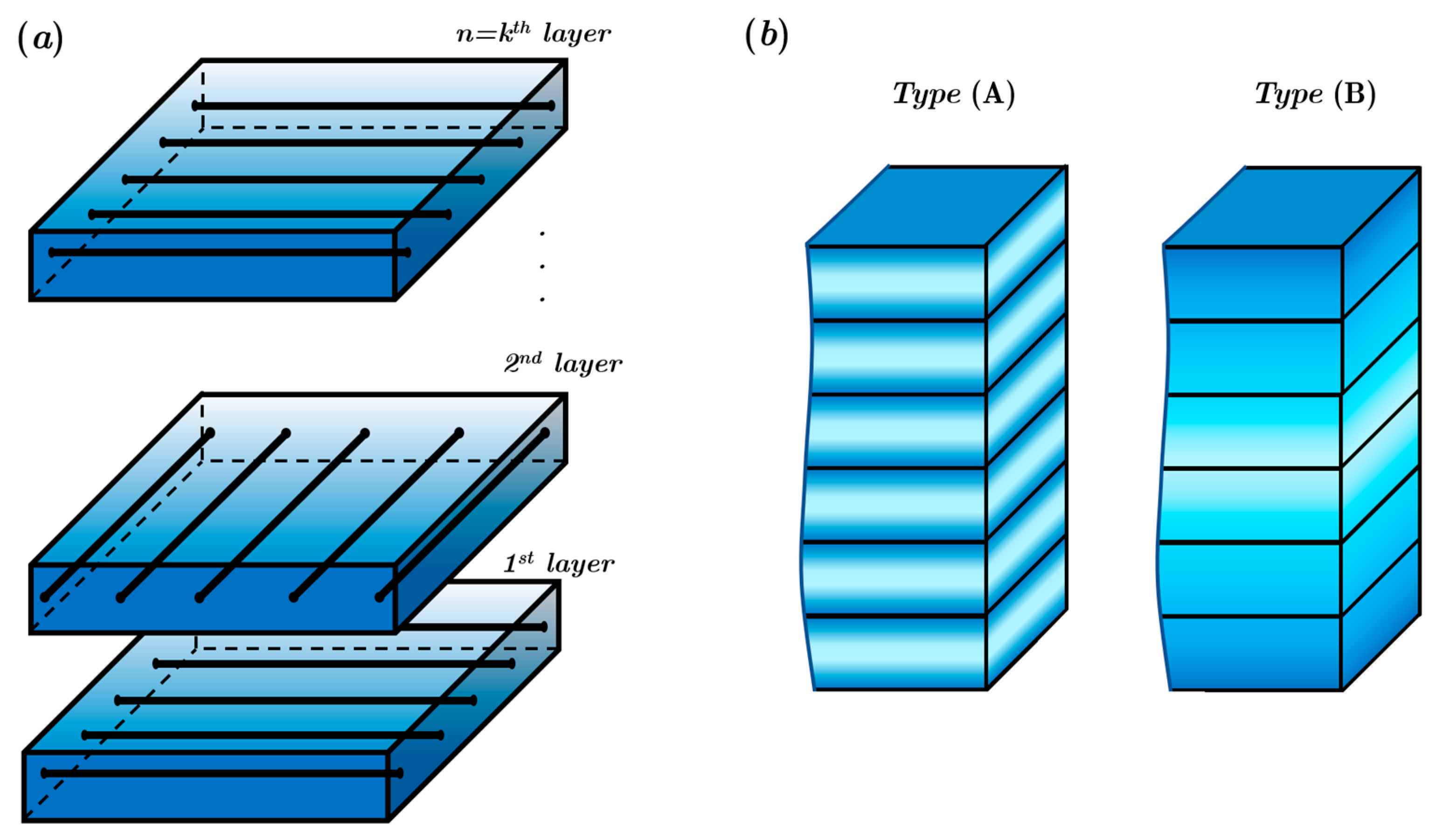
This manuscript aims, for the first time, to investigate the impact of the length scale, as well as the microstructure, on the natural frequencies of sandwich FG-CNTRC nonlocal strain gradient of nanoshell, using kinematic higher-order hyperbolic shear function. Two types of material distribution and four gradations (UN, X, O, and V) are proposed and presented in Section 2. The problem formulation, constitutive equations, variational statement, and equations of motion are derived in Section 3 and Section 4. The analytical solution of the governing equations of motion is derived in Section 5. The accuracy of the developed procedure is verified and discussed in Section 6. In Section 7, detailed parametric studies are performed and discussed to highlight the effect of the CNT distribution pattern, the thickness and the stretching, the geometry of the plate/shell, the boundary conditions, the total number of layers, the length scale and material scale parameters, on the natural frequencies. The conclusion and main points are summarized in Section 8.

2. Material and Geometrical Modeling

A rectangular multilayer shell in the Cartesian coordinate system, (x, y, z) is shown in Figure 1. The shell has a curved length, a, width, b, and thickness h. The principal radii of curvature of the mid-plane in x is Rx, and Ry in the y direction. The shell is reinforced by single wall carbon nanotubes (SWCNTs). All sheets of the shell have the same thickness. Four different patterns of CNT distribution are presented in this study, which are a uniform distribution UD and three functionally graded distributions, FG-X FG-V and FG-O. Two types of cross-ply multilayer CNTRC shells are proposed.

2.1. CNTRC Structure Type (A): CNTRC(A)

In Type (A), each layer has self-distribution (UD, X, O or V) (as shown in Figure 2). The effective material properties of CNT-reinforced composite shell are obtained based on a micromechanical model following [60].
UD distribution pattern:
V c n t = V c n t *
FG-X distribution Pattern:
V c n t = 2 ( | 2 | z | | z ( k 1 ) + z ( k ) | | z ( k ) z ( k 1 ) ) p V c n t *
FG-O distribution Pattern:
V c n t = 2 ( 1 ( | 2 | z | | z ( k 1 ) + z ( k ) | | z ( k ) z ( k 1 ) ) p ) V c n t *
FG-V distribution Pattern:
V c n t = 2 ( 1 2 ( 2 z z ( k ) z ( k 1 ) 2 ( z ( k ) z ( k 1 ) ) ) ) p V c n t *
V c n t   and   V c n t * refer, respectively, to the volume fraction and the total volume fraction of CNTs, p is the inhomogeneity material graduation index,   k denotes the layer number.

2.2. CNTRC Structure Type (B): CNTRC(B)

In this type, the distribution of CNTs is applied along the total thickness (see Figure 2). The effective material properties of CNTRC shell are defined as
FG-X distribution Pattern:
V c n t = 2 ( 2 | z | h ) p V c n t *
FG-O distribution Pattern:
V c n t = 2 ( 1 2 | z | h ) p V c n t *
FG-V distribution Pattern:
V c n t = ( 1 + 2 z h ) p V c n t *

3. Kinematics and Kinetics Relations

Within this section, the kinematics and kinetics relations are presented. Hyperbolic sine function shear deformation theory is applied in this analysis to satisfy the zero-shear stress at the free outer boundaries. Based on the higher-order hyperbolic shear function, the displacement field is given as, [61]
u ( x , y , z , t ) = ( 1 + z R x ) u 0 z w 0 x + f ( z ) ψ x v ( x , y , z , t ) = ( 1 + z R y ) v 0 z w 0 y + f ( z ) ψ y w ( x , y , z , t ) = w 0
The displacements of the midplane of the composite plate are u 0 , v 0 , and w 0 , whereas ψ x and ψ y are the rotations of the transverse normal at the middle surface z = 0. The proposed hyperbolic sine shape function, f ( z ) can be written as
f ( z ) = h sinh ( z h ) 3 z 3 2 h 2
The strain displacement relations can be obtained by derivative of the displacements as
{ ε x x ε y y γ x y } = { ε x x 0 ε y y 0 γ x y 0 } + z { ε x x 1 ε y y 1 γ x y 1 } + f ( z ) { ε x x 2 ε y y 2 γ x y 2 } ε z z = 0 ,   { γ y z γ x z } = d f ( z ) d z { γ y z 0 γ x z 0 } ,
where εxx, εyy, γxy, are, respectively, the normal and shear strain component, while ε x x 0 ,   ε y y 0 ,   γ x y 0 , ε x x 2 ,   ε y y 2 ,   γ x y 2 ,   γ y z 0 ,   and   γ x z 0 are related to the midplane displacement and rotaion deriviatives and rotation as follows:
{ ε x x 0 ε y y 0 γ x y 0 } = { u 0 x + w 0 R x v 0 y + w 0 R y v 0 x + u 0 y } ,   { ε x x 1 ε y y 1 γ x y 1 } = { 2 w 0 x 2 2 w 0 y 2 2 2 w 0 x y } ,   { ε x x 2 ε y y 2 γ x y 2 } = { φ 1 x φ 2 y φ 2 x + φ 1 y } ,   { γ y z 0 γ x z 0 } = { φ x φ y } .
The stresses relations of kth layer accounting for both nonlocal elastic stress field and the strain gradient stress field, can be written as [38]
[ 1 μ 2 ] { σ x x σ y y τ y z τ x z τ x y } ( k ) = [ 1 λ 2 ] [ Q ¯ 11 k Q ¯ 12 k 0 Q ¯ 12 k Q ¯ 22 k 0 0 0 0 0 0 0 Q ¯ 44 k 0 0 0 0 0 Q ¯ 55 k 0 0 0 0 0 Q ¯ 66 k ] { ε x x ε y y γ y z γ x z γ x y } ( k )
Here, μ denote the nonlocal parameter and λ is the length scale parameter and 2 denotes the Laplacian operator [62]. The transformed material constants Q ¯ i j k are expressed as:
Q ¯ 11 k = Q 11 c o s 4 θ k + 2 ( Q 12 + 2 Q 66 ) s i n 2 θ k c o s 2 θ k + Q 22 s i n 4 θ k Q ¯ 12 k = ( Q 11 + Q 22 4 Q 66 ) s i n 2 θ k c o s 2 θ k + Q 12 ( s i n 4 θ k + c o s 4 θ k ) Q ¯ 22 k = Q 11 s i n 4 θ k + 2 ( Q 12 + 2 Q 66 ) s i n 2 θ k c o s 2 θ k + Q 22 c o s 4 θ k Q ¯ 66 k = ( Q 11 + Q 22 2 Q 12 2 Q 66 ) s i n 2 θ k c o s 2 θ k + Q 66 ( s i n 4 θ k + c o s 4 θ k ) Q ¯ 44 k = Q 44 c o s 2 θ k + Q 55 s i n 2 θ k Q ¯ 55 k = Q 55 c o s 2 θ k + Q 44 s i n 2 θ k
where θ k is the lamination angle ( θ k = 0 ° ,   90 ° ) and
Q 11 = E 11 1 ν 12 ν 21 ,   Q 22 = E 22 1 ν 12 ν 21 ,   Q 12 = ν 12 E 22 1 ν 12 ν 21 , Q 44 = G 23 ,   Q 55 = G 13 ,   Q 66 = G 12
The stress relations, moment and additional moment resultants can be obtained by integration of Equation (12), which will result
[ 1 μ 2 ] { { N } { M } { P } } = [ 1 λ 2 ] [ [ A ] [ B ] [ C ] [ B ] [ D ] [ F ] [ C ] [ F ] [ H ] ] { { ε 0 } { ε 1 } { ε 2 } }
[ 1 μ 2 ] { R y z R x z } = [ 1 λ 2 ] [ J 44 J 45 J 45 J 55 ] { γ y z 0 γ x z 0 }
where
{ N } = { N x x N y y N x y } T ,   { M } = { M x x M y y M x y } T ,   { P } = { P x x P y y P x y } T { ε 0 } = { ε x x 0 ε y y 0 γ x y 0 } T ,   { ε 1 } = { ε x x 1 ε y y 1 γ x y 1 } T ,   { ε 2 } = { ε x x 2 ε y y 2 γ x y 2 } T
The coefficients A i j ,   B i j , D i j , C i j , F i j and H i j can be defined as
{ A i j ,   B i j ,   D i j ,   C i j , F i j , H i j } = n = 1 n h n 1 h n Q i j ( n ) { 1 ,   z , z 2 , f ( z ) , z f ( z ) , f ( z ) 2 } d z ,   ( i , j = 1 , 2 , 6 ) J i i = n = 1 n h n 1 h n Q i i ( n ) [ d f ( z ) d z ] 2 d z , ( i = 4 , 5 )

4. Dynamic Equations of Motion

To derive the equations of motion of the CNTRC shell, Hamilton’s principle is utilized:
t 2 t 1 δ ( U T + V ) d t = 0
The virtual strain energy of the CNTRC shell, δ ( U ) can be determined as
δ U p = 1 2 V [ σ x x ( k ) δ ε x x + σ y y ( k ) δ ε x x + σ x y ( k ) δ γ x y + σ x z ( k ) δ γ x z + σ y z ( k ) δ γ y z ] d V
At any moment, the virtual kinetic energy of the CNTRC shell, δ T can be stated as
δ T = 1 2 0 L A ρ ( u ˙ δ u ˙ + v ˙ δ v ˙ + w ˙ δ w ˙ ) d A d x
δ T = V { I 0 ( u ˙ 0 δ u ˙ 0 + v ˙ 0 δ v ˙ 0 + w ˙ 0 δ w ˙ 0 ) + I 1 ( w ˙ 0 x δ u ˙ 0 + w ˙ 0 y δ v ˙ 0 + u ˙ 0 δ w ˙ 0 x + v ˙ 0 δ w ˙ 0 y ) # + I 2 ( w ˙ 0 x δ w ˙ 0 x + w ˙ 0 y δ w ˙ 0 y ) + I 3 ( φ ˙ x δ u ˙ 0 + u ˙ 0 δ φ ˙ x + φ ˙ y δ v ˙ 0 + v ˙ 0 δ φ ˙ y ) + I 4 ( φ ˙ x δ w ˙ 0 x + w ˙ 0 x δ φ ˙ x + φ ˙ y δ w ˙ 0 y + w ˙ 0 y δ φ ˙ y ) + I 5 ( φ ˙ x δ φ ˙ x + φ ˙ y δ φ ˙ y ) } d x d y d z
where
{ I 0 ,   I 1 ,   I 2 ,   I 3 , I 4 , I 5 } = n = 1 k ρ ( z ) { 1 ,   z , z 2 , Φ ( z ) , z Φ ( z ) , ( Φ ( z ) ) 2 } d z
Neglecting the effect of the external applied load, insertion of Equations (20) and (22), into Equation (19), the equilibrium equations for CNTRC shells can be obtained as follows:
[ 1 μ 2 ] [ A 11 2 u 0 x 2 + A 66 2 u 0 y 2 + ( A 12 + A 66 ) 2 v 0 x y + ( A 11 R x + A 12 R y ) w 0 x B 11 3 w 0 x 3 ( B 12 + 2 B 66 ) 3 w 0 x y 2 + B 11 S 2 ψ x x 2 + B 66 S 2 ψ x y 2 + ( B 12 S + B 66 S ) 2 ψ y x y ] = [ 1 λ 2 ] [ ( I 0 + 2 I 1 R x + I 3 R y 2 ) 2 u 0 t 2 ( I 1 + I 2 R x ) 2 w 0 x t 2 + ( I 3 + I 4 R x ) 2 ψ x t 2 ]
[ 1 μ 2 ] [ ( A 12 + A 66 ) 2 u 0 x y + A 22 2 v 0 y 2 + A 66 2 v 0 x 2 ( B 11 + 2 B 66 ) 3 w 0 x 2 y B 22 3 w 0 y 3 + ( A 12 R x + A 22 R y ) w 0 x + ( B 12 S + B 66 S ) 2 ψ x x y + B 22 S 2 ψ y y 2 + B 66 S 2 ψ y x 2 ] = [ 1 λ 2 ] [ ( I 0 + 2 I 1 R y + I 2 R y 2 ) 2 v 0 t 2 ( I 1 + I 2 R y ) 3 w 0 y t 2 + ( I 3 + I 4 R y ) 2 ψ y t 2 ]
[ 1 μ 2 ] [ B 11 3 u 0 x 3 + ( B 12 + 2 B 66 ) 3 u 0 x y 2 ( A 11 R x + A 12 R y ) u 0 x + ( B 12 + 2 B 66 ) 3 v 0 x 2 y + B 22 3 v 0 y 3 ( A 12 R x + A 22 R y ) v 0 y + ( 2 B 11 R x + 2 B 12 R y ) 2 w 0 x 2 D 11 4 w 0 x 4 ( 2 D 12 + 4 D 66 ) 4 w 0 x 2 y 2 D 22 4 w 0 y 4 + ( 2 B 12 R x + 2 B 22 R y ) 2 w 0 y 2 ( A 11 R x 2 + 2 A 12 R x R y + A 22 R y 2 ) w 0 + D 11 S 3 ψ x x 3 + ( D 12 S + 2 D 66 S ) 3 ψ x x y 2 ( B 11 S R x + B 12 S R y ) ψ x x + ( D 12 S + 2 D 66 S ) 3 ψ y x 2 y + D 22 S 3 ψ y y 3 ( B 12 S R x + B 22 S R y ) ψ y y ] = [ 1 λ 2 ] [ I 0 2 w 0 t 2 + ( I 1 + I 2 R x ) 3 u 0 x t 2 + ( I 1 + I 2 R y ) 3 v 0 y t 2 I 2 ( 4 w 0 x 2 t 2 + 4 w 0 y 2 t 2 ) + I 4 ( 3 ψ x x t 2 + 3 ψ y y t 2 ) ]
[ 1 μ 2 ] [ B 11 S 2 u 0 x 2 + B 66 S 2 u 0 y 2 + ( B 12 S + B 66 S ) 2 v 0 x y u 0 x D 11 S 3 w 0 x 3 ( D 12 S + 2 D 66 S ) 3 w 0 x y 2 + ( B 11 S R x + B 12 S R y ) w 0 x + F 11 S 2 ψ x x 2 + F 66 S 2 ψ x y 2 A 44 S ψ x + ( F 12 S + F 66 S ) 2 ψ y x y ] = [ 1 λ 2 ] [ ( I 3 + I 4 R x ) 2 u 0 t 2 I 4 3 w 0 x t 2 + I 5 2 ψ x t 2 ]
[ 1 μ 2 ] [ ( B 12 S + B 66 S ) 2 u 0 x y + B 11 S 2 v 0 y 2 + B 66 S 2 v 0 x 2 ( D 12 S + 2 D 66 S ) 3 w 0 x 2 y D 22 S 3 w 0 y 3 + ( B 12 S R x + B 22 S R y ) w 0 x + ( F 12 S + F 66 S ) 2 ψ x x y + F 11 S 2 ψ y y 2 + F 66 S 2 ψ y x 2 A 44 S ψ y ] = [ 1 λ 2 ] [ ( I 3 + I 4 R y ) 2 v 0 t 2 I 4 3 w 0 y t 2 + I 5 2 ψ y t 2 ]

5. Analytical Solution

Within this section, closed forms are presented for the eigen value problem of the free vibration of the CNTRC shells considering different boundary conditions including: simple-simple (SSSS), clamped-clamped (CCCC), clamped-simple-clamped-simple (CSCS), clamped-clamped-simple-simple (CCSS), clamped-simple-simple-simple (CSSS), clamped-clamped-clamped-simple (CCCS). The Galerkin approach is employed to provide accurate closed-form solutions. Based on the Galerkin technique, the expressions for generalized displacements are as follows:
{ u 0 , ψ x } = m = 1 n = 1 { U m n , X m n } X m ( x ) x Y n ( y ) e i ω t { v 0 , ψ y } = m = 1 n = 1 { V m n , Z m n } X m ( x ) Y n ( y ) y e i ω t w 0 = m = 1 n = 1 W m n X m ( x ) Y n ( y ) e i ω t
U m n , V m n , X m n   and Z m n are arbitrary parameters. The functions X m ( x ) and Y n ( y ) that satisfy the above boundary conditions are given in Table 1.
Where λ = m π / a , μ = n π / b . m and n are mode numbers. By substituting Equation (29) in Equations (24)–(28), one obtains
[ [ K ] 5 × 5 ω n m 2 [ M ] 5 × 5 ] { Δ } = 0   [ K ] = [ K 11 K 12 K 13 K 14 K 15 K 12 K 22 K 23 K 24 K 25 K 13 K 23 K 33 K 34 K 35 K 14 K 24 K 34 K 44 K 45 K 15 K 25 K 35 K 45 K 55 ] ,   [ M ] = [ M 11 M 12 M 13 M 14 M 15 M 21 M 22 M 23 M 24 M 25 M 13 M 23 M 33 M 34 M 35 M 14 M 24 M 34 M 44 M 45 M 15 M 25 M 35 M 45 M 55 ]
where ω 2   and   { Δ }   are, respectively, the eigen values and the eigen vectors. [ K ]   and   [ M ] are, respectively, the rigidity and mass matrices. The elements K i j and M i j of the matrix [K] and [M] are given in Appendix A.

6. Verification of the Developed Procedure

The accuracy of the proposed procedure will be checked in this section. The developed procedure is applied to obtain results for the free vibration of functionally graded plates and shells. For the straight plate, the radii of curvature are R x / a = R y / b = , and R x / a = R y / b = 5 for the spherical shell, R x / a = 5 and R y / b = for the cylindrical shell, R x / a = 5 and R y / b = 5 for the hyperbolic-paraboloid shell, R x / a = 5 and R y / b = 7.5 for the elliptical-paraboloid shell (see Figure 3). The obtained results are compared with those generated in the literature using various solution techniques, as shown in Figure 4. The material characteristics used for verification are as follows: alumina (AlO2) as ceramic with material properties; ( E c = 380   GPa , ρ c = 3800   kg / m 3 ) and aluminium (Al) as metal with the following characteristics: ( E m = 70   GPa , ρ c = 2707   kg / m 3 ). Poisson’s ratio is taken as υ = 0.3 . Comparison between results shows good agreement verifiying the accuracy of the developed procedure.

7. Results and Discussions

Considering a CNTRC nanoshell in a high-temperature medium. The temperature field is assumed to be uniform over the nanoshell. The (10,10) single-walled carbon nanotubes (SWCNT) are utilized as reinforcements. The effective temperature-dependent material properties of the CNTs are given as the following expression [62]
P = P 0 ( P 1 T 1 + 1 + P 1 T + P 2 T 2 + P 3 T 3 )
Here, T = T 0 + Δ T , where T 0 is the ambient temperature ( T 0 = 300 K ) and Δ T is the temperature difference. P 0 , P 1 , P 2 , and P 3 are the temperature coefficients given in Table 2.
Young’s modulus of the polymeric matrix (PmPV) is dependent on the temperature and can be expressed as:
E m [ GPa ] = ( 3.51 0.0047 T )
The Poisson ratio and the mass density are independent of the temperature and given as: v m = 0.34 and ρ m = 1150 kg / m 3 , respectively.
To standardize and simplify calculations, the normalized parameters for the vibration analyses of CNTRC shells are described using the following forms:
ω ¯ = ω h ρ m E m
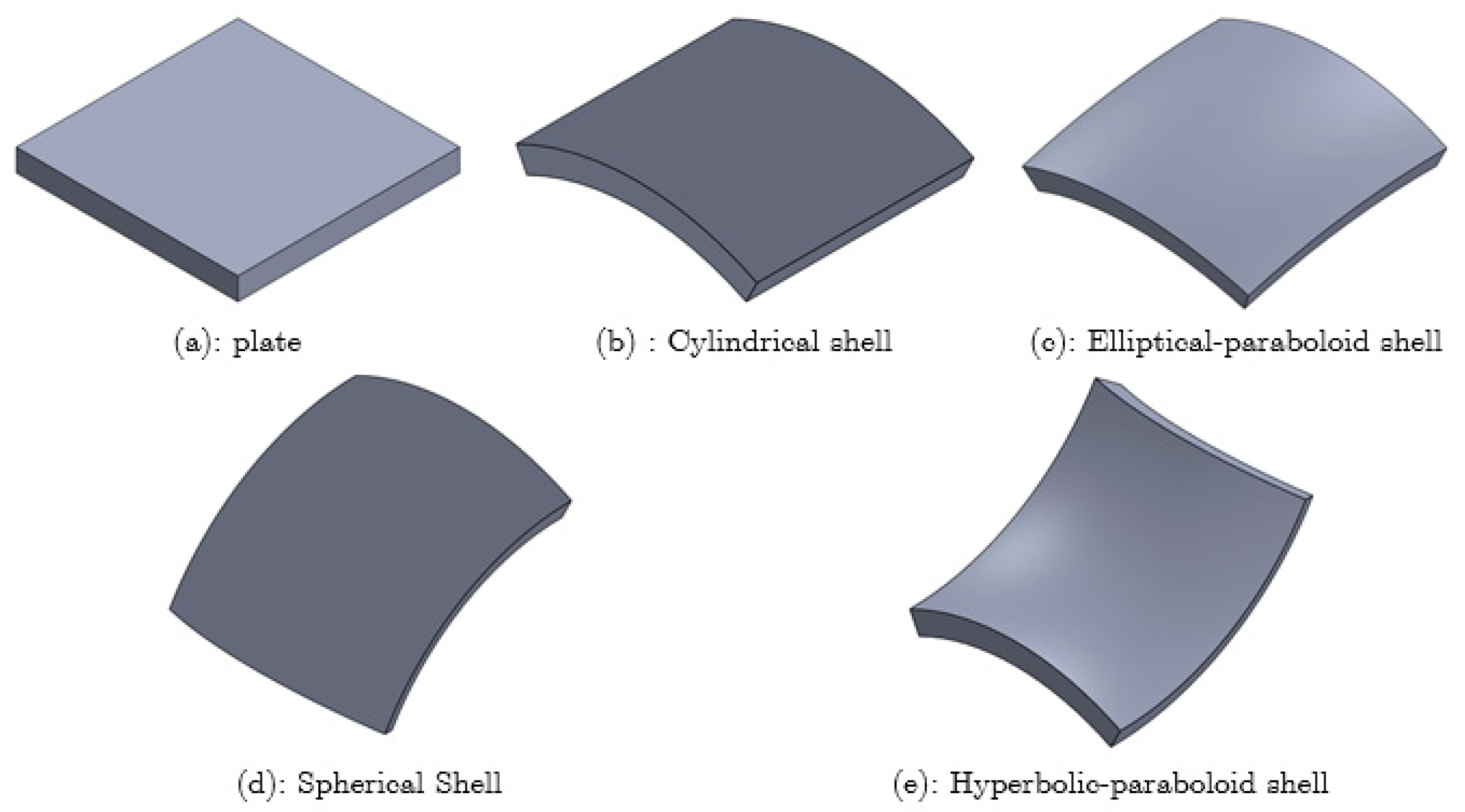
In the following study, a parametric analysis of the vibration of CNTRC shells was carried out. As mentioned in the previous section, two types of laminated shells are proposed: CNTRC(A) and CNTRC(B). For the straight plate, the radii of curvature are R x / a = R y / b = , and R x / a = R y / b = 5 for the spherical shell, R x / a = 5 and R y / b = for the cylindrical shell, R x / a = 5 and R y / b = 5 for the hyperbolic-paraboloid shell, R x / a = 5 and R y / b = 7.5 for the elliptical-paraboloid shell (Figure 3).
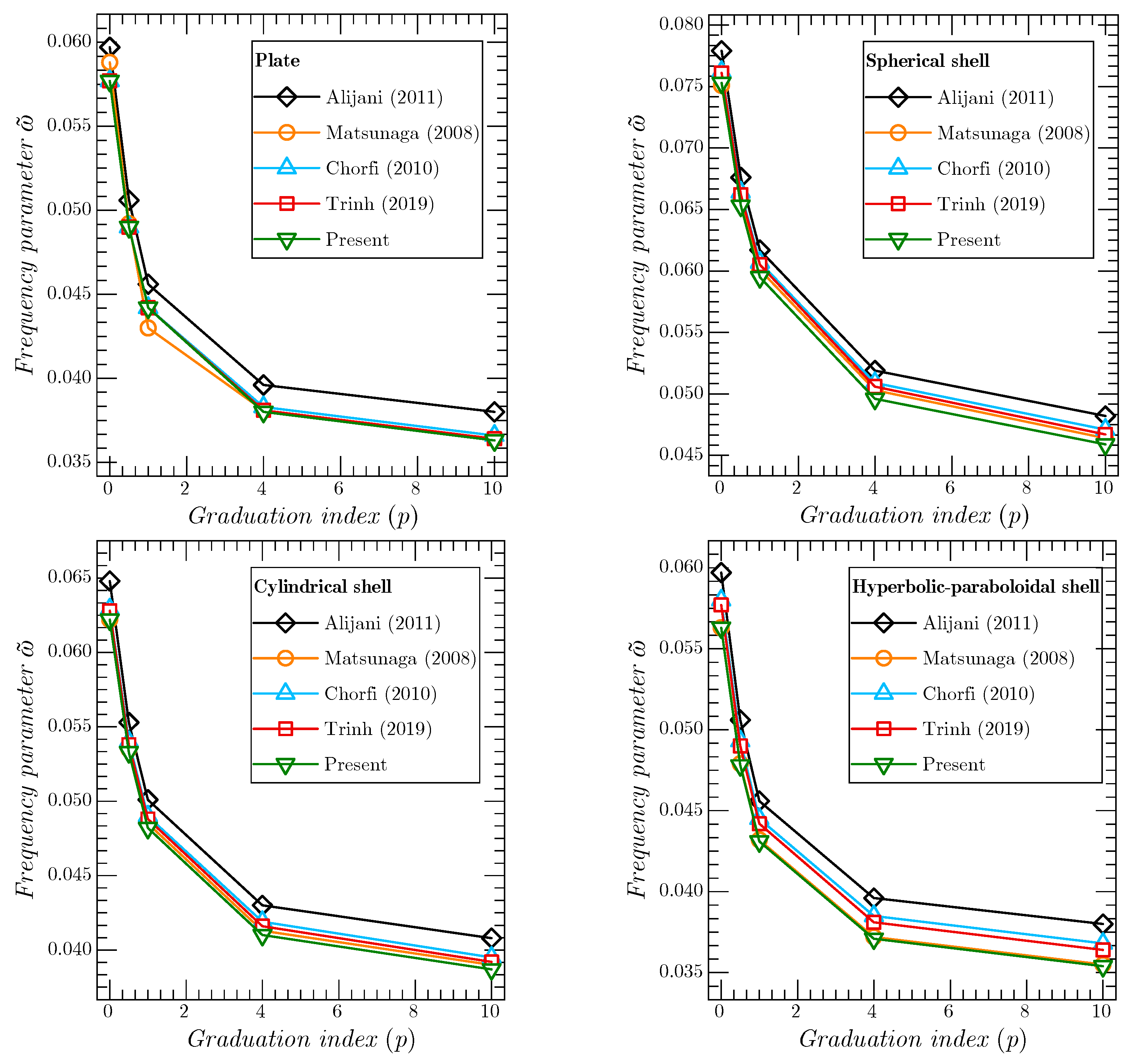
The effect of CNTRC type and CNT distribution patterns on the dimensionless frequency of CNTRC shells for various inhomogeneity material index p is illustrated in Table 3. Increase in the material parameter p leads to decrement in dimensionless frequencies.
In Table 4, we analyse the impact of the number of layers and CNT distribution patterns on the dimensionless frequency of CNTRC shells. In general, increase in the number of layers leads to increment in the dimensionless frequency and the stiffness of the plate. The FG–X CNTRC(B) shells have the highest values of dimensionless frequencies.
In Table 5, the influence of a change in temperature on the dimensionless frequency of different types and patterns of simply supported CNTRC shells is investigated. The stiffness of the CNTRC shell reduces with increase in temperature.
The action of the geometric parameters (a/h and b/a) on the dimensionless frequency of various types of simply supported spherical CNTRC shells is shown in Table 6. It is observed that the frequencies increase by increasing both the thickness ratio a/h and the aspect ratio b/a.
Table 7 presents the impact of the nonlocal and length scale parameters on the dimensionless frequency of simply supported spherical nanoshell. It is clear that the value of the frequency reduces by decreasing the length scale parameter and increasing the nonlocal parameter.
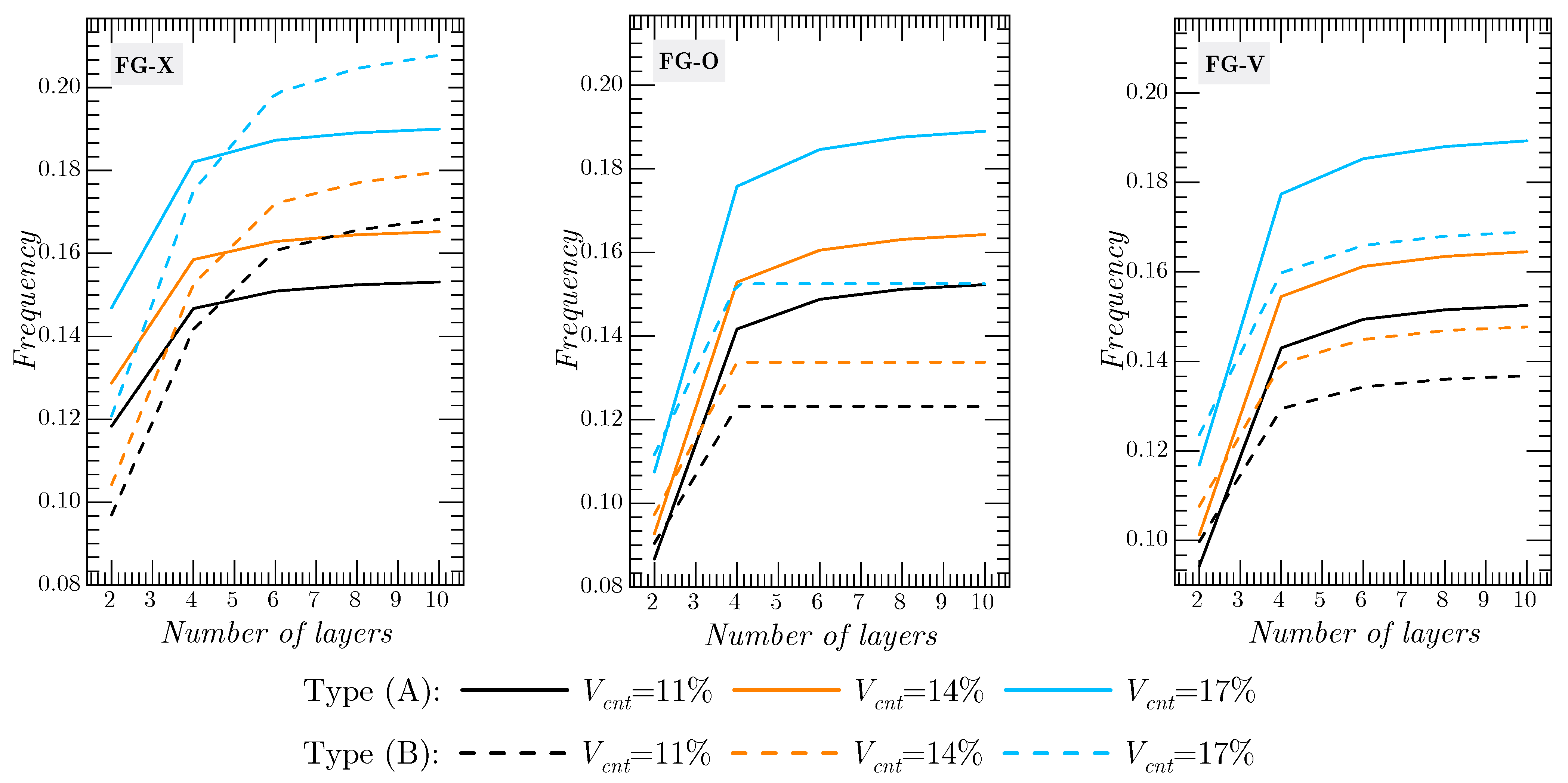
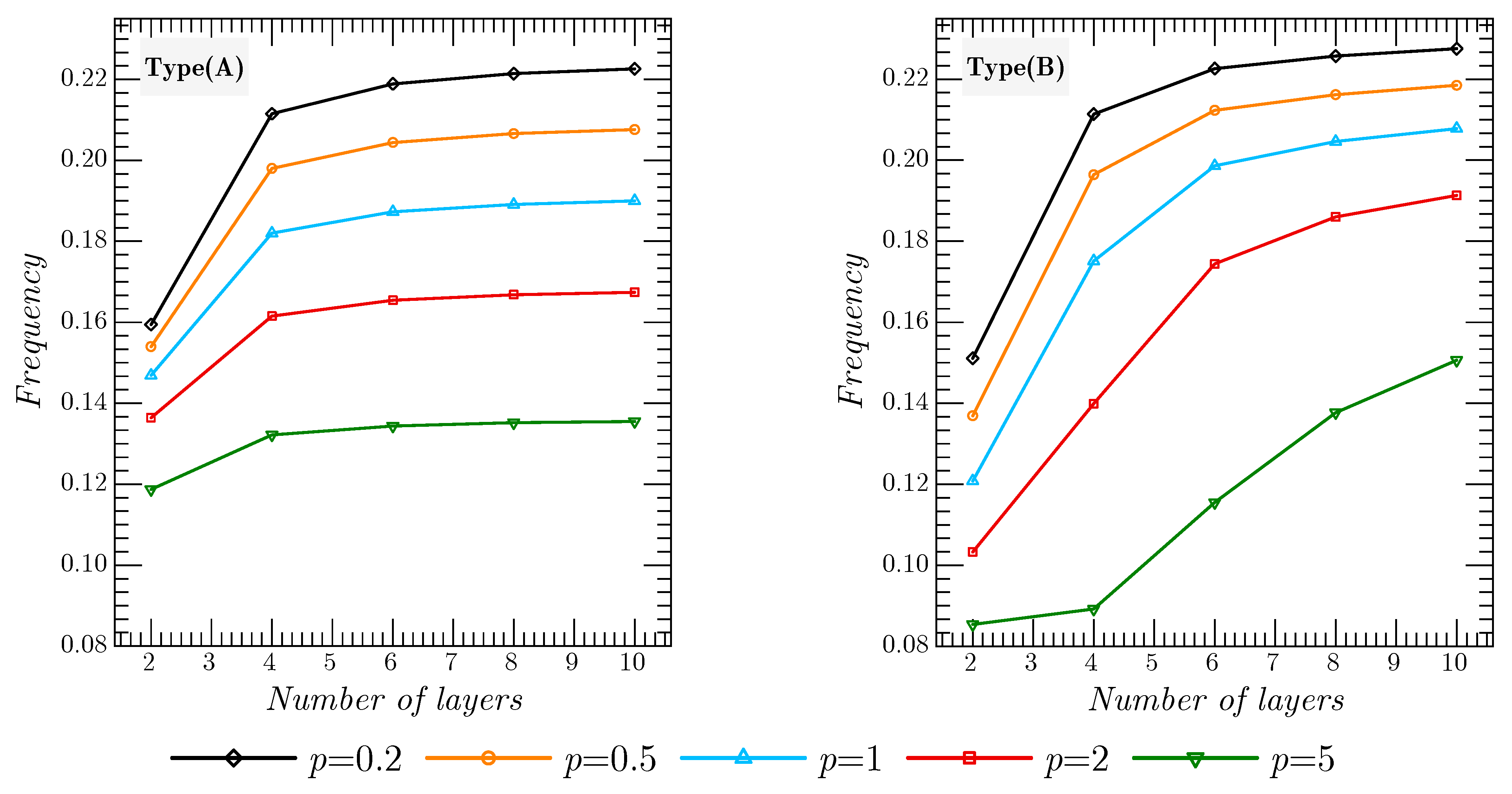
To understand the impact of the number of layers and to view the advantages of the proposed structure, Figure 5 is presented. Clearly, as shown in these figures, increase in the number of layers produces a stiffer structure. Comparing the two structure types, the CNTRC structure Type (B) in distribution FG-X has the highest stiffness, and therefore an increment in the dimensionless frequency. In addition, as is known, increase in the volume fraction V c n t * increases the rigidity of the structure regardless of the CNTRC type and the CNT distribution. The use of more than two layers in the case of FG–O CNTRC(B) barely changes the frequency values, whatever the volume fraction.
In Figure 6, we plotted the dimensionless frequencies of two types of simply supported CNTRC plates with FG-X distribution as a function of the number of layers and the inhomogeneity material parameter p. Through these curves, we can clearly see that the material parameter p has a significant effect on the CNTRC(B) plates, more so than the CNTRC(A).
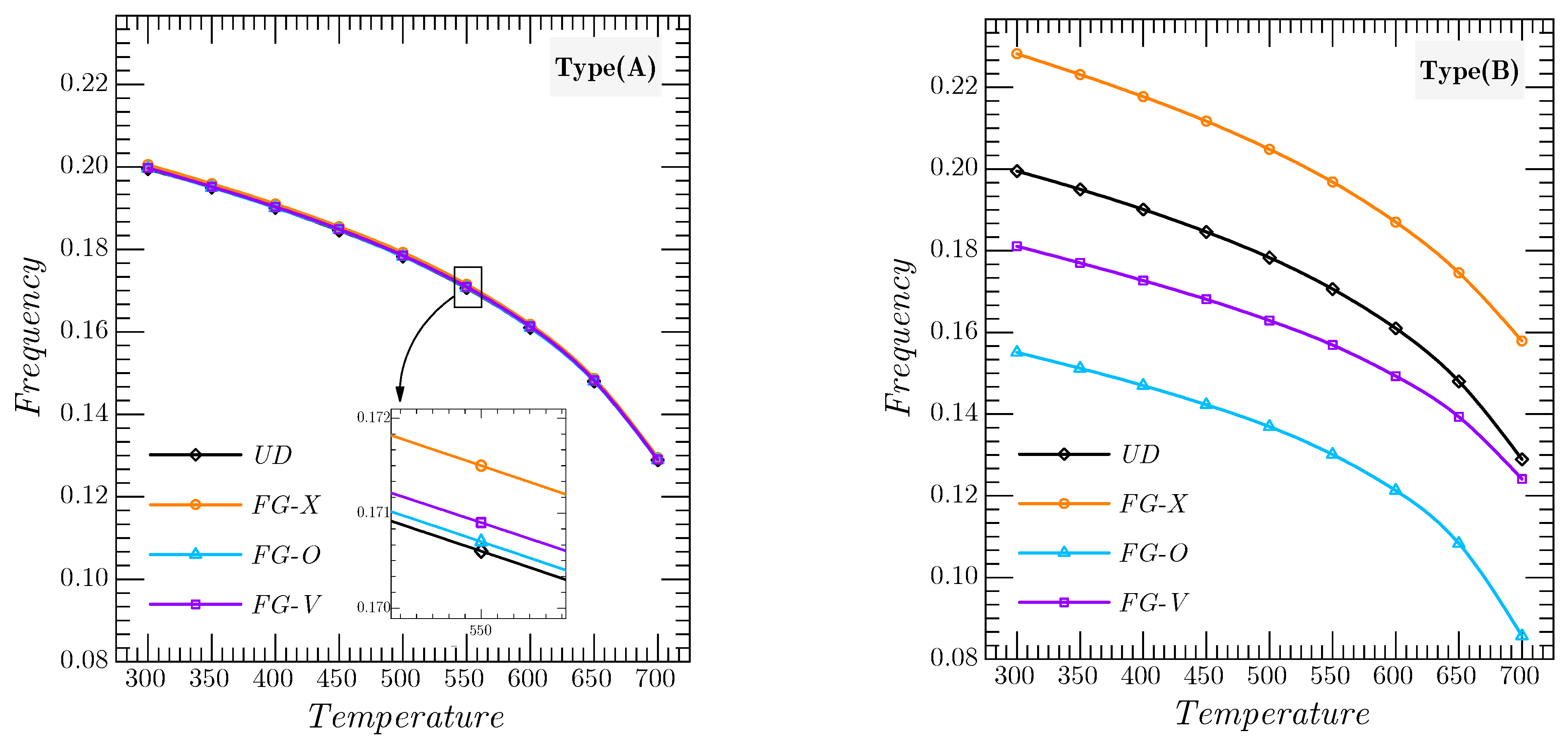
High temperature reduces the stiffness of the structure by affecting the material properties. Figure 7 presents an examination of the impact of the thermal environment on the vibrational response of the two types of simply supported spherical CNTRC shell for various CNT distribution patterns. Because of the even distribution of CNTs in each layer (10 layers) of CNTRC(A) structures, we obtained similar results, and, therefore, we conclude that the CNT distribution pattern has almost no influence on the mechanical response, unlike the CNTRC(B) shell. In addition, increase in the temperature leads to a decrement in the rigidity of the CNTRC shell, and thus, the dimensionless frequency decreases.
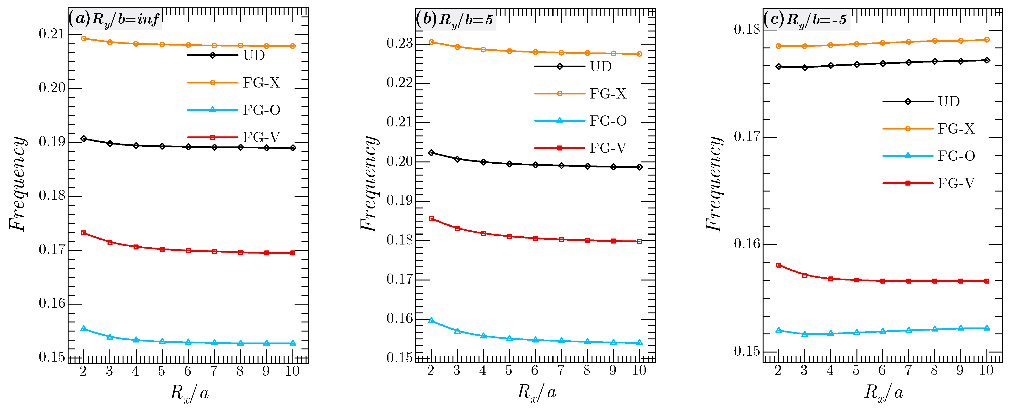
In Figure 8, we show the radii of curvature ( R x / a ) on the dimensionless frequencies of CNTRC(B) shells by fixing the radii of curvature R y / b at inf, 5 and −5. In the case of the cylindrical shell and the elliptical-paraboloid shells (R/b = inf, 5), the augmentation of the radii of curvature R x / a leads to a decrement in frequencies for the values R x / a 5 , whatever the CNT distribution pattern is, and then the results are almost constant.
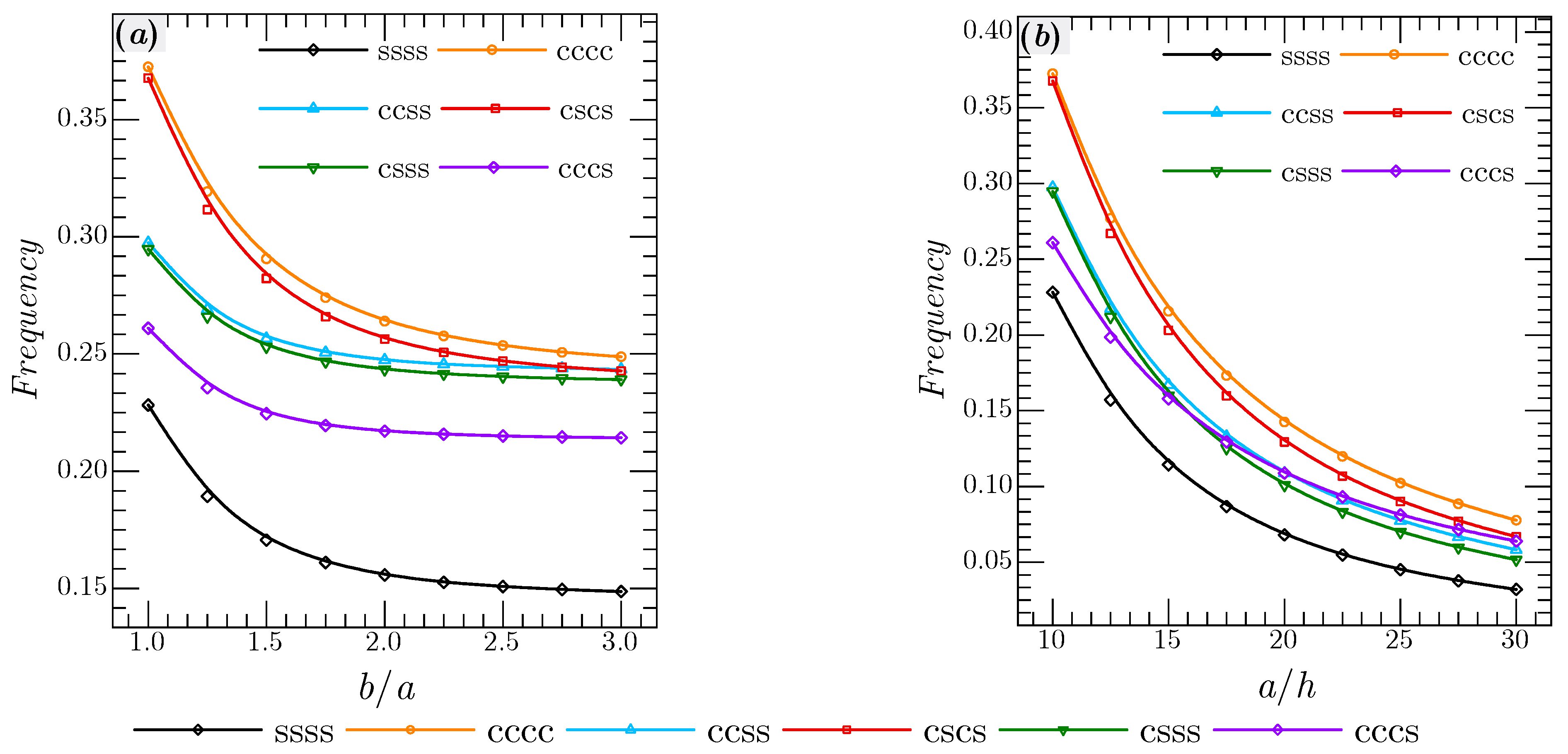
The impact of various boundary conditions and the geometry of the CNTRC(B) plate (b/a and a/h) on the frequencies is plotted in Figure 9. The dimensionless frequencies decrease with decrease in the thickness ratio a/h. For the aspect ratio b/a effect, the frequencies decrease critically for values b / a 2 . In addition, the fully clamped shells have the highest values of frequency, while the lowest values are for the simply supported one.
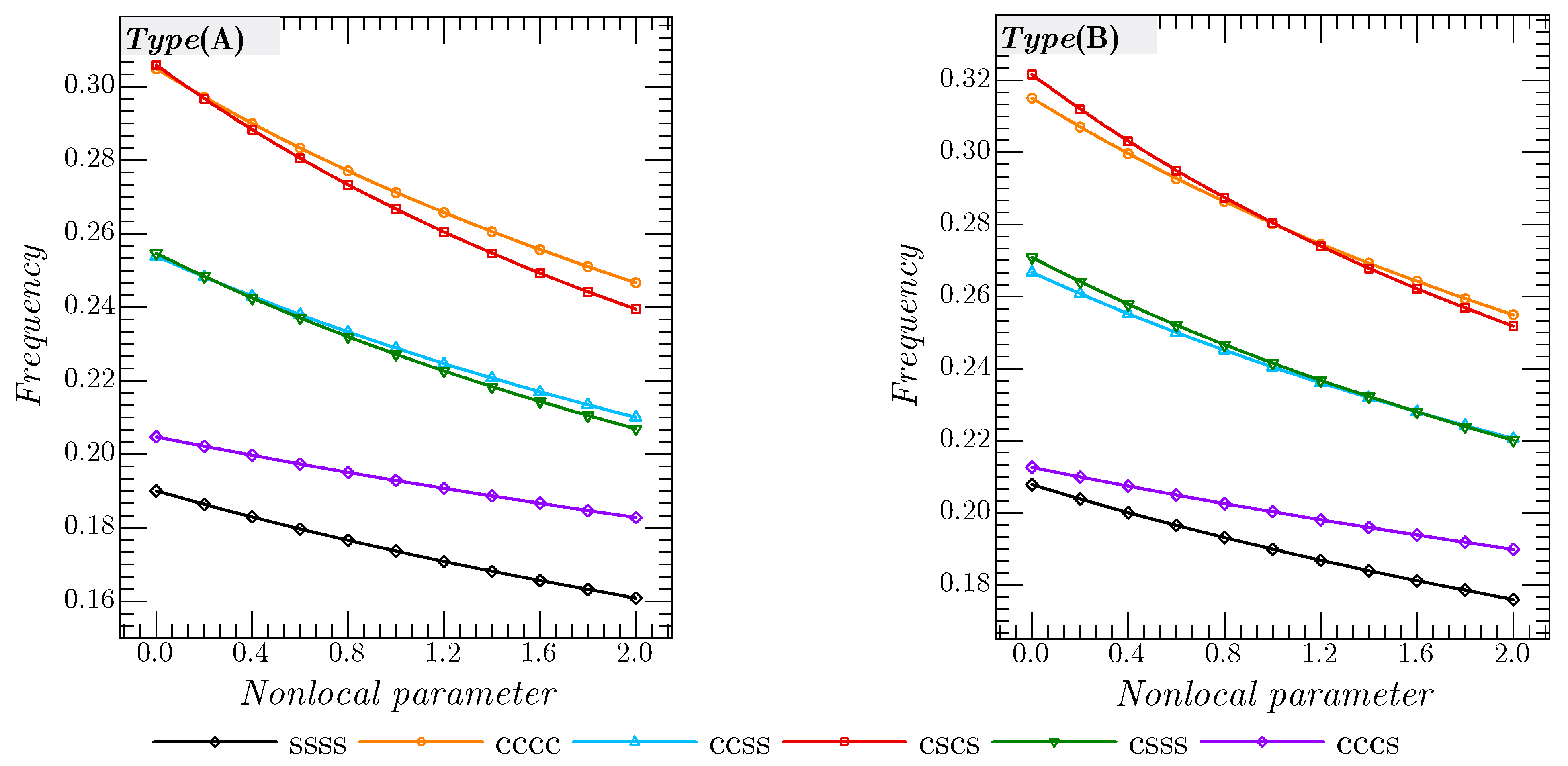
To show the nonlocality effect on the dimensionless frequency of the two types of CNTRC spherical shell for various boundary conditions, Figure 10 curves are plotted. The nonlocal parameter 
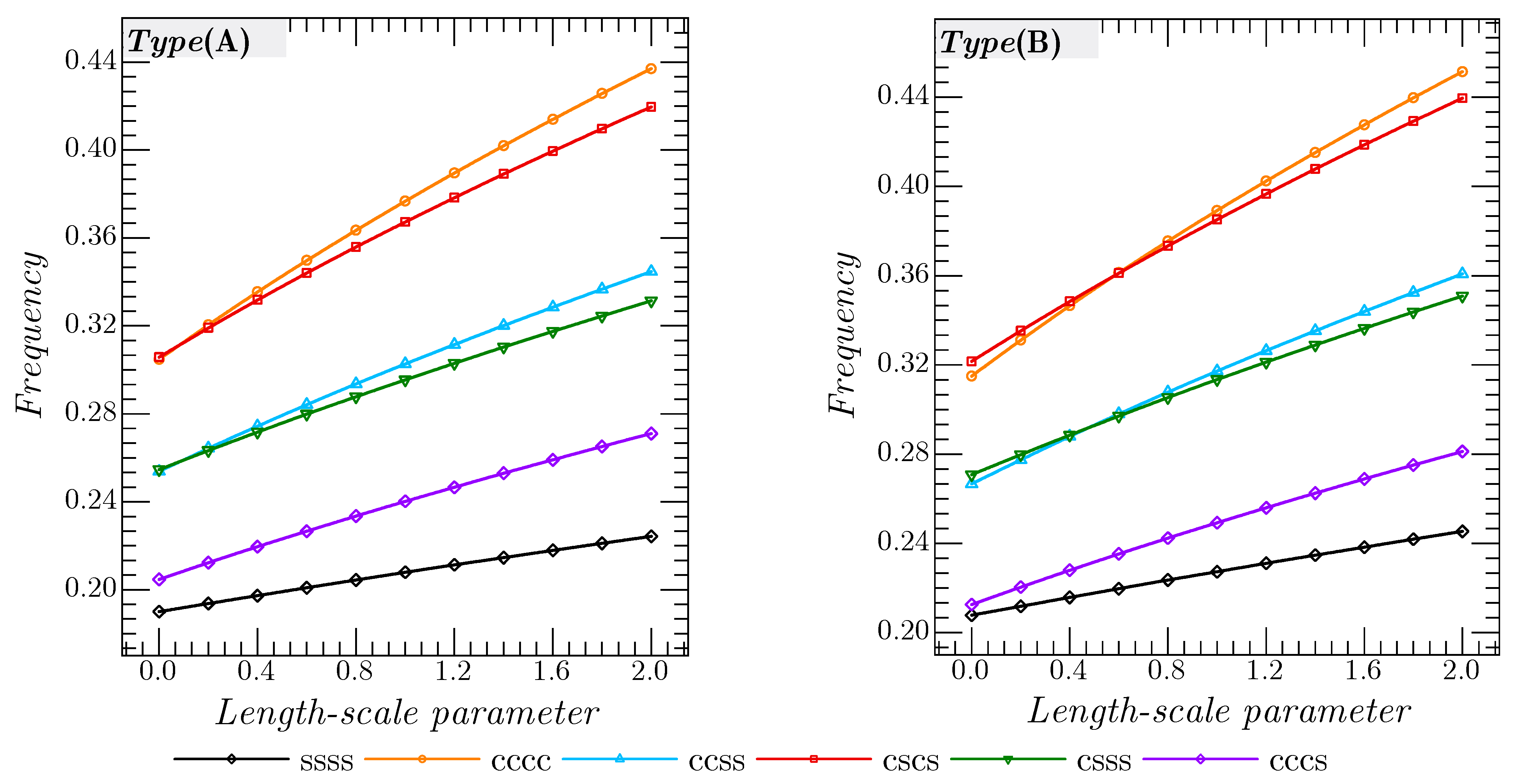
μ is changed from 0 to 2. Regardless of either the CNTRC type or the boundary conditions, it is seen from this figure that the inclusion of the nonlocal parameter reduces the plate stiffness, and therefore decreases the dimensionless frequencies. Unlike the nonlocal parameter effect, in Figure 11, it is observed that the dimensionless frequency decreases with increase in the length-scale parameter.

8. Conclusions

This paper presents a modified mathematical continuum model to investigate the free vibration response of FG-CNTRC nanoshell with temperature-dependent material properties. The length scale and microstructure influences are employed in the model by using nonlocal strain gradient theory. The Galerkin approach is implemented to solve the system of equations and obtain the analytical solution. Numerical studies are performed to present the CNT distribution pattern, the thickness stretching, the geometry of the plate/shell, boundary conditions, the total number of layers, the length scale and material scale parameters on the vibrational frequencies of CNTRC laminated nanoplates and nanoshells. The main findings can be summarized as: -
  • Increase in the material gradation parameter p leads to decrement in dimensionless frequencies.
  • The material parameter p has a significant effect on the CNTRC(B) plates, more than the CNTRC(A).
  • Increase in the volume fraction V c n t * increases the rigidity of the structure regardless of the CNTRC type and the CNT distribution
  • Increase in the number of layers leads to increment in the dimensionless frequency and the stiffness of the plate. The FG–X CNTRC(B) shells have the highest values of dimensionless frequencies.
  • Based on the geometric parameters, the frequencies increase by increasing both the thickness ratio a/h and the aspect ratio b/a. For the aspect ratio b/a effect, the frequencies decrease critically for values of b / a 2 .
  • In the case of the cylindrical shell, the elliptical-paraboloid shells (R/b = inf, 5), the augmentation of the radii of curvature R x / a leads to a decrement in frequencies for the values R x / a 5 whatever the CNT distribution pattern is, and then the results are almost constant.
  • The fully clamped shells have the highest values of frequency, while the lowest values are for the simply supported one.
  • For size-length and microstructure scales, the value of the frequency reduces by decreasing the length scale parameter and increasing the nonlocal parameter.

Author Contributions

A.M. (project administration, funding acquisition, data curation); A.A.D. (software, validation, formal analysis, investigation); M.B. (formal analysis, investigation); A.W.A. (software, visualization, data curation); R.O. (Conceptualization, methodology, formal analysis); K.H.A. (software, investigation, resources); M.A.H. (methodology, review and editing); A.A. (methodology, software, validation); M.A.E. (Conceptualization, methodology, review and editing). All authors have read and agreed to the published version of the manuscript.

Funding

This research was funded by the Institutional Fund Projects under Grant no. (IFPRC-012-135-2020).

Institutional Review Board Statement

Not applicable.

Informed Consent Statement

Not applicable.

Data Availability Statement

Not applicable.

Acknowledgments

This research was funded by institutional Fund Projects under grant no. (IFPRC-012-135-2020). The authors gratefully acknowledge the technical and financial support from the Ministry of Education and King Abdulaziz University, Jeddah, Saudi Arabia.

Conflicts of Interest

The authors declare no conflict of interest.

Appendix A

Rigidity matrix elements;
K 11 = A 11 0 a 0 b 3 X m x 3 Y n X m x Y n d x d y + A 66 0 a 0 b X m x 2 Y n y 2 X m x Y n d x d y λ [ ( A 11 + A 66 ) 0 a 0 b 3 X m x 3 2 Y n y 2 X m x Y n d x d y + A 11 0 a 0 b 5 X m x 5 Y n X m x Y n d x d y + A 66 0 a 0 b X m x 4 Y n y 4 X m x Y n d x d y ]
K 12 = ( A 12 + A 66 ) ( 0 a 0 b X m x 2 Y n y 2 X m x Y n d x d y λ [ 0 a 0 b 3 X m x 3 2 Y n y 2 X m x Y n d x d y + 0 a 0 b X m x 4 Y n y 4 X m x Y n d x d y ] )
K 13 = ( A 11 R x + A 12 R y ) ( 0 a 0 b X m x Y n X m x Y n d x d y λ [ 0 a 0 b 3 X m x 3 Y n X m x Y n d x d y + 0 a 0 b X m x 2 Y n y 2 X m x Y n d x d y ] ) B 11 0 a 0 b 3 X m x 3 Y n X m x Y n d x d y ( B 12 + 2 B 66 ) 0 a 0 b X m x 2 Y n y 2 X m x Y n d x d y λ [ ( B 12 + 2 B 66 + B 11 ) 0 a 0 b 3 X m x 3 2 Y n y 2 X m x Y n d x d y B 11 0 a 0 b 5 X m x 5 Y n X m x Y n d x d y ]
K 14 = B 11 s 0 a 0 b 3 X m x 3 Y n X m x Y n d x d y + B 66 s 0 a 0 b X m x 2 Y n y 2 X m x Y n d x d y λ [ ( B 11 s + B 66 s ) 0 a 0 b 3 X m x 3 2 Y n y 2 X m x Y n d x d y + B 11 s 0 a 0 b 5 X m x 5 Y n X m x Y n d x d y + B 66 s 0 a 0 b X m x 4 Y n y 4 X m x Y n d x d y ]
K 15 = ( B 12 s + B 66 s ) ( 0 a 0 b X m x 2 Y n y 2 X m x Y n d x d y λ [ 0 a 0 b 3 X m x 3 2 Y n y 2 X m x Y n d x d y + 0 a 0 b X m x 4 Y n y 4 X m x Y n d x d y ] )
K 21 = ( A 12 + A 66 ) ( 0 a 0 b 2 X m x 1 Y n y X m Y n y d x d y λ [ 0 a 0 b 4 X m x 4 Y n y X m Y n y d x d y + 0 a 0 b 2 X m x 2 3 Y n y 3 X m Y n y d x d y ] )
K 22 = A 22 0 a 0 b X m 3 Y n y 3 X m Y n y d x d y + A 66 0 a 0 b 0 b 2 X m x 2 Y n y X m Y n y d x d y λ [ ( A 22 + A 66 ) 0 a 0 b 2 X m x 2 3 Y n y 3 X m Y n y d x d y + A 22 0 a 0 b X m 5 Y n y 5 X m Y n y d x d y + A 66 0 a 4 X m x 4 Y n y X m Y n y d x d y ]
K 23 = ( A 12 R x + A 22 R y ) ( 0 a 0 b X m Y n y X m Y n y d x d y λ [ 0 a 0 b 2 X m x 2 Y n y X m Y n y d x d y + 0 a 0 b X m 3 Y n y 3 X m Y n y d x d y ] ) B 22 0 a 0 b X m 3 Y n y 3 X m Y n x d x d y ( B 12 + 2 B 66 ) 0 a 0 b 2 X m x 2 Y n x X m Y n x d x d y λ ( ( B 22 + B 12 + 2 B 66 ) 0 a 0 b 2 X m x 2 3 Y n y 3 X m Y n x d x d y ( B 12 + 2 B 66 ) 0 a 0 b 4 X m x 4 Y n x X m Y n x d x d y B 22 0 a 0 b X m 5 Y n y 5 X m Y n x d x d y )
K 24 = ( B 12 s + B 66 s ) ( 0 a 0 b 2 X m x 2 Y n y X m Y n y d x d y λ [ 0 a 0 b 4 X m x 4 Y n y X m Y n y d x d y + 0 a 0 b 2 X m x 2 3 Y n y 3 X m Y n y d x d y ] )
K 25 = B 22 s 0 a 0 b X m 3 Y n y 3 X m Y n y d x d y + B 66 s 0 a 0 b 2 X m x 2 Y n y X m Y n y d x d y λ [ ( B 22 s + B 66 s ) 0 a 0 b 2 X m x 2 3 Y n y 3 X m Y n y d x d y + B 66 s 0 a 0 b 4 X m x 4 Y n y X m Y n y d x d y + B 22 s 0 a 0 b X m 5 Y n y 5 X m Y n y d x d y ]
K 31 = ( A 11 R x + A 12 R y ) ( 0 a 0 b 2 X n x 2 Y n X m Y n d x d y λ [ 0 a 0 b 4 X n x 4 Y n X m Y n d x d y + 0 a 0 b 2 X n x 2 2 Y n y 2 X m Y n d x d y ] ) + B 11 0 a 0 b 4 X n x 4 Y n X m Y n d x d y + ( B 12 + 2 B 66 ) 0 a 0 b 2 X m x 2 2 Y n y 2 X m Y n d x d y λ [ B 11 0 a 0 b 6 X n x 6 Y n X m Y n d x d y + ( B 11 + B 12 + 2 B 66 ) 0 a 0 b 4 X m x 4 2 Y n y 2 X m Y n d x d y + ( B 12 + 2 B 66 ) 0 a 0 b 2 X m x 2 4 Y n y 4 X m Y n d x d y ]
K 32 = ( A 12 R x + A 22 R y ) ( 0 a 0 b X m 2 Y n y 2 X m Y n d x d y λ [ 0 a 0 b 2 X m x 2 2 Y n y 2 X m Y n d x d y + 0 a 0 b X m 4 Y n y 4 X m Y n d x d y ] ) + B 22 0 a 0 b X m 4 Y n y 4 X m Y n d x d y + ( B 12 + 2 B 66 ) 0 a 0 b 2 X m x 2 2 Y n y 2 X m Y n d x d y λ [ ( B 22 + B 12 + 2 B 66 ) 0 a 0 b 2 X m x 2 4 Y n y 4 X m Y n d x d y + ( B 12 + 2 B 66 ) 0 a 0 b 4 X m x 4 2 Y n y 2 X m Y n d x d y + B 22 0 a 0 b X m 6 Y n y 6 X m Y n d x d y ]
K 33 = 2 ( B 11 R x + B 12 R y ) ( 0 a 0 b 2 X n x 2 Y n X m Y n d x d y λ [ 0 a 0 b 4 X m x 4 Y n X m Y n d x d y + 0 a 0 b 2 X n x 2 2 Y n y 2 X m Y n d x d y ] ) + 2 ( B 12 R x + B 22 R y ) ( 0 a 0 b X m 2 Y n y 2 X m Y n d x d y λ [ 0 a 0 b 2 X m x 2 2 Y n y 2 X m Y n d x d y + 0 a 0 b X m 4 Y n y 4 X m Y n d x d y ] ) ( A 11 R x 2 + 2 A 12 R x R y + A 22 R y 2 ) ( 0 a 0 b X m Y n X m Y n d x d y λ [ 0 a 0 b 2 X m x 2 Y n X m Y n d x d y + 0 a 0 b X m 2 Y n y 2 X m Y n d x d y ] ) D 11 0 a 0 b 4 X m x 4 Y n X m Y n d x d y D 22 0 a 0 b X m 4 Y n y 4 X m Y n d x d y 2 ( D 12 + 2 D 66 ) 0 a 0 b 2 X m x 2 2 Y n y 2 X m Y n d x d y λ [ D 11 0 a 0 b 6 X m x 6 Y n X m Y n d x d y D 22 0 a 0 b 2 X m x 2 4 Y n y 4 X m Y n d x d y 2 ( D 12 + 2 D 66 ) 0 a 0 b 4 X m x 4 2 Y n y 2 X m Y n d x d y D 11 0 a 0 b 4 X m x 4 2 Y n y 2 X m Y n d x d y D 22 0 a 0 b X m 6 Y n y 6 X m Y n d x d y 2 ( D 12 + 2 D 66 ) 0 a 0 b 2 X m x 2 4 Y n y 4 X m Y n d x d y ]
K 34 = ( B 11 s R x + B 12 s R y ) ( 0 a 0 b 2 X n x 2 Y n X m Y n d x d y λ [ 0 a 0 b 4 X m x 4 Y n X m Y n d x d y + 0 a 0 b 2 X n x 2 2 Y n y 2 X m Y n d x d y ] ) + D 11 s 0 a 0 b 4 X m x 4 Y n X m Y n d x d y + ( D 12 s + 2 D 66 s ) 0 a 0 b 2 X m x 2 2 Y n y 2 X m Y n d x d y λ [ D 11 s 0 a 0 b 6 X m x 6 Y n X m Y n d x d y + ( D 11 s + D 12 s + 2 D 66 s ) 0 a 0 b 4 X m x 4 2 Y n y 2 X m Y n d x d y + ( D 12 s + 2 D 66 s ) 0 a 0 b 2 X m x 2 4 Y n y 4 X m Y n d x d y ]
K 35 = ( B 12 s R x + B 22 s R y ) ( 0 a 0 b X m 2 Y n y 2 X m Y n d x d y λ [ 0 a 0 b 2 X m x 2 2 Y n y 2 X m Y n d x d y + 0 a 0 b X m 4 Y n y 4 X m Y n d x d y ] ) + D 22 s 0 a 0 b X m 4 Y n y 4 X m Y n d x d y + ( D 12 s + 2 D 66 s ) 0 a 0 b 2 X m x 2 2 Y n y 2 X m Y n d x d y λ [ ( D 12 s + 2 D 66 s ) 0 a 0 b 4 X m x 4 2 Y n y 2 X m Y n d x d y + D 22 s 0 a 0 b X m 6 Y n y 6 X m Y n d x d y + ( D 22 s + D 12 s + 2 D 66 s ) 0 a 0 b 2 X m x 2 4 Y n y 4 X m Y n d x d y ]
K 41 = B 11 s 0 a 0 b 3 X m x 3 Y n X m x Y n d x d y + B 66 s 0 a 0 b X m x 2 Y n y 2 X m x Y n d x d y λ [ B 11 s 0 a 0 b 5 X m x 5 Y n X m x Y n d x d y + ( B 11 s + B 66 s ) 0 a 0 b 3 X m x 3 2 Y n y 2 X m x Y n d x d y + B 66 s 0 a 0 b X m x 4 Y n y 4 X m x Y n d x d y ]
K 42 = ( B 12 s + B 66 s ) ( 0 a 0 b X m x 2 Y n y 2 X m x Y n d x d y λ [ 0 a 0 b 3 X m x 3 2 Y n y 2 X m x Y n d x d y + 0 a 0 b X m x 4 Y n y 4 X m x Y n d x d y ] )
K 43 = ( B 11 s R x + B 12 s R y ) ( 0 a 0 b X m x Y n X m x Y n d x d y λ [ 0 a 0 b 3 X m x 3 Y n X m x Y n d x d y + 0 a 0 b X m x 2 Y n y 2 X m x Y n d x d y ] ) D 11 s 0 a 0 b 3 X m x 3 Y n X m x Y n d x d y ( D 12 s + 2 D 66 s ) 0 a 0 b X m x 2 Y n y 2 X m x Y n d x d y λ [ ( D 11 s + D 12 s + 2 D 66 s ) 0 a 0 b 3 X m x 3 2 Y n y 2 X m x Y n d x d y D 11 s 0 a 0 b 5 X m x 5 Y n X m x Y n d x d y ( D 12 s + 2 D 66 s ) 0 a 0 b X m x 4 Y n y 4 X m x Y n d x d y ]
K 44 = F 11 s 0 a 0 b 3 X m x 3 Y n X m x Y n d x d y + F 66 s 0 a 0 b X m x 2 Y n y 2 X m x Y n d x d y A 44 s 0 a 0 b X m x Y n X m x Y n d x d y λ [ F 11 s 0 a 0 b 5 X m x 5 Y n X m x Y n d x d y + ( F 66 s + F 11 s ) 0 a 0 b 3 X m x 3 2 Y n y 2 X m x Y n d x d y A 44 s 0 a 0 b 3 X m x 3 Y n X m x Y n d x d y + F 66 s 0 a 0 b X m x 4 Y n y 4 X m x Y n d x d y A 44 s 0 a 0 b X m x 2 Y n y 2 X m x Y n d x d y ]
K 45 = ( F 12 s + F 66 s ) ( 0 a 0 b X m x 2 Y n y 2 X m x Y n d x d y λ [ 0 a 0 b 3 X m x 3 2 Y n y 2 X m x Y n d x d y + 0 a 0 b X m x 4 Y n y 4 X m x Y n d x d y ] )
K 51 = ( B 12 s + B 66 s ) 0 a 0 b 2 X m x 2 Y n y X m Y n y d x d y λ [ 0 a 0 b 4 X m x 4 Y n y X m Y n y d x d y + 0 a 0 b 2 X m x 2 3 Y n y 3 X m Y n y d x d y ]
K 52 = B 22 s 0 a 0 b X m 3 Y n y 3 X m Y n y d x d y + B 66 s 0 a 0 b 2 X m x 2 Y n y X m Y n y d x d y λ ( ( B 22 s + B 66 s ) 0 a 0 b 2 X m x 2 3 Y n y 3 X m Y n y d x d y + B 66 s 0 a 0 b 4 X m x 4 Y n y X m Y n y d x d y + B 22 s 0 a 0 b X m 5 Y n y 5 X m Y n y d x d y )
K 53 = ( B 12 s R x + B 22 s R y ) ( 0 a 0 b X m Y n y X m Y n y d x d y λ [ 0 a 0 b 2 X m x 2 Y n y X m Y n y d x d y + 0 a 0 b X m 3 Y n y 3 X m Y n y d x d y ] ) D 22 s 0 a 0 b X m 3 Y n y 3 X m Y n y d x d y ( D 12 s + 2 D 66 s ) 0 a 0 b 2 X m x 2 Y n y X m Y n y d x d y λ [ ( D 12 s + 2 D 66 s ) 0 a 0 b 4 X m x 4 Y n y X m Y n y d x d y D 22 s 0 a 0 b X m 5 Y n y 5 X m Y n y d x d y ( D 22 s + D 12 s + 2 D 66 s ) 0 a 0 b 2 X m x 2 3 Y n y 3 X m Y n y d x d y ]
K 54 = ( F 12 s + F 66 s ) ( 0 a 0 b 2 X m x 2 Y n y X m Y n y d x d y λ [ 0 a 0 b 4 X m x 4 Y n y X m Y n y d x d y + 0 a 0 b 2 X m x 2 3 Y n y 3 X m Y n y d x d y ] )
K 55 = F 22 s 0 a 0 b X m 3 Y n y 3 X m Y n y d x d y + F 66 s 0 a 0 b 2 X m x 2 Y n y X m Y n y d x d y A 55 s 0 a 0 b X m Y n y X m Y n y d x d y λ ( ( F 22 s + F 66 s ) 0 a 0 b 2 X m x 2 3 Y n y 3 X m Y n y d x d y + F 66 s 0 a 0 b 4 X m x 4 Y n y X m Y n y d x d y A 55 s 0 a 0 b 2 X m x 2 Y n y X m Y n y d x d y + F 22 s 0 a 0 b X m 5 Y n y 5 X m Y n y d x d y A 44 s 0 a 0 b X m 3 Y n y 3 X m Y n y d x d y )
Mass matrix elements;
M 11 = ( I 0 + 2 I 1 R x + I 3 R y 2 ) ( 0 a 0 b X m x Y n X m x Y n d x d y μ [ 0 a 0 b 3 X m x 3 Y n X m x Y n d x d y + 0 a 0 b X m x 2 Y n y 2 n X m x Y n d x d y ] )
M 13 = ( I 1 + I 2 R x ) ( 0 a 0 b X m x Y n X m x Y n d x d y μ [ 0 a 0 b 3 X m x 3 Y n X m x Y n d x d y + 0 a 0 b X m x 2 Y n y 2 n X m x Y n d x d y ] )
M 14 = ( I 3 + I 4 R x ) ( 0 a 0 b X m x Y n X m x Y n d x d y μ [ 0 a 0 b 3 X m x 3 Y n X m x Y n d x d y + 0 a 0 b X m x 2 Y n y 2 n X m x Y n d x d y ] )
M 22 = ( I 0 + 2 I 1 R y + I 2 R y 2 ) ( 0 a 0 b X m Y n y X m Y n y d x d y μ [ 0 a 0 b 2 X m x 2 Y n y X m Y n y d x d y + 0 a 0 b X m 3 Y n y 3 X m Y n y d x d y ] )
M 23 = ( I 1 + I 2 R y ) ( 0 a 0 b X m Y n y X m Y n y d x d y μ [ 0 a 0 b 2 X m x 2 Y n y X m Y n y d x d y + 0 a 0 b X m 3 Y n y 3 X m Y n y d x d y ] )
M 25 = ( I 3 + I 4 R y ) 0 a 0 b X m Y n y X m Y n y d x d y
M 31 = ( I 1 + I 2 R x ) ( 0 a 0 b 2 X m x 2 Y n X m Y n d x d y μ [ 0 a 0 b 4 X m x 4 Y n X m Y n d x d y + 0 a 0 b 2 X m x 2 2 Y n y 2 X m Y n d x d y ] )
M 32 = ( I 1 + I 2 R y ) ( 0 a 0 b X m 2 Y n y 2 X m Y n d x d y μ [ 0 a 0 b 2 X m x 2 2 Y n y 2 X m Y n d x d y + 0 a 0 b X m 4 Y n y 4 X m Y n d x d y ] )
M 33 = I 0 ( 0 a 0 b X m Y n X m Y n d x d y μ [ 0 a 0 b 2 X m x 2 Y n X m Y n d x d y + 0 a 0 b X m 2 Y n y 2 X m Y n d x d y ] ) I 2 ( 0 a 0 b 2 X m x 2 Y n X m Y n d x d y μ [ 0 a 0 b 4 X m x 4 Y n X m Y n d x d y + 2 0 a 0 b 2 X m x 2 2 Y n y 2 X m Y n d x d y ] + 0 a 0 b X m 2 Y n y 2 X m Y n d x d y μ 0 a 0 b X m 4 Y n y 4 X m Y n d x d y )
M 34 = I 4 ( 0 a 0 b 2 X m x 2 Y n X m Y n d x d y μ [ 0 a 0 b 4 X m x 4 Y n X m Y n d x d y + 0 a 0 b 2 X m x 2 2 Y n y 2 X m Y n d x d y ] )
M 35 = I 4 ( 0 a 0 b X m 2 Y n y 2 X m Y n d x d y μ [ 0 a 0 b 2 X m x 2 2 Y n y 2 X m Y n d x d y + 0 a 0 b X m 4 Y n y 4 X m Y n d x d y ] )
M 41 = ( I 3 + I 4 R x ) ( 0 a 0 b X m x Y n X m x Y n d x d y μ [ 0 a 0 b 3 X m x 3 Y n X m x Y n d x d y + 0 a 0 b X m x 2 Y n y 2 X m x Y n d x d y ] )
M 43 = I 4 ( 0 a 0 b X m x Y n X m x Y n d x d y μ [ 0 a 0 b 3 X m x 3 Y n X m x Y n d x d y + 0 a 0 b X m x 2 Y n y 2 X m x Y n d x d y ] )
M 44 = I 5 ( 0 a 0 b X m x Y n X m x Y n d x d y μ [ 0 a 0 b 3 X m x 3 Y n X m x Y n d x d y + 0 a 0 b X m x 2 Y n y 2 X m x Y n d x d y ] )
M 52 = ( I 3 + I 4 R y ) ( 0 a 0 b X m Y n y X m Y n y d x d y μ [ 0 a 0 b 2 X m x 2 Y n y X m Y n y d x d y + 0 a 0 b X m 3 Y n y 3 X m Y n y d x d y ] )
M 53 = I 4 ( 0 a 0 b X m Y n y X m Y n y d x d y μ [ 0 a 0 b 2 X m x 2 Y n y X m Y n y d x d y + 0 a 0 b X m 3 Y n y 3 X m Y n y d x d y ] )
M 12 = M 15 = M 21 = M 24 = M 42 = M 45 = M 51 = M 54 = M 55 = 0

References

  1. Eltaher, M.A.; El-Borgi, S.; Reddy, J.N. Nonlinear analysis of size-dependent and material-dependent nonlocal CNTs. Compos. Struct. 2016, 153, 902–913. [Google Scholar] [CrossRef]
  2. Eltaher, M.A.; Agwa, M.A. Analysis of size-dependent mechanical properties of CNTs mass sensor using energy equivalent model. Sens. Actuators A Phys. 2016, 246, 9–17. [Google Scholar] [CrossRef]
  3. Avey, M.; Fantuzzi, N.; Sofiyev, A.H.; Kuruoglu, N. Nonlinear vibration of multilayer shell-type structural elements with double curvature consisting of CNT patterned layers within different theories. Compos. Struct. 2021, 275, 114401. [Google Scholar] [CrossRef]
  4. Zhu, P.; Lei, Z.X.; Liew, K.M. Static and free vibration analyses of carbon nanotube-reinforced composite plates using finite element method with first order shear deformation plate theory. Compos. Struct. 2012, 94, 1450–1460. [Google Scholar] [CrossRef]
  5. Garg, A.; Chalak, H.D.; Zenkour, A.M.; Belarbi, M.O.; Sahoo, R. Bending and free vibration analysis of symmetric and unsymmetric functionally graded CNT reinforced sandwich beams containing softcore. Thin-Walled Struct. 2022, 170, 108626. [Google Scholar] [CrossRef]
  6. Zhang, L.W.; Song, Z.G.; Liew, K.M. State-space Levy method for vibration analysis of FG-CNT composite plates subjected to in-plane loads based on higher-order shear deformation theory. Compos. Struct. 2015, 134, 989–1003. [Google Scholar] [CrossRef]
  7. Song, Z.G.; Zhang, L.W.; Liew, K.M. Active vibration control of CNT reinforced functionally graded plates based on a higher-order shear deformation theory. Int. J. Mech. Sci. 2016, 105, 90–101. [Google Scholar] [CrossRef]
  8. Singh, S.D.; Sahoo, R. Static and free vibration analysis of functionally graded CNT reinforced composite plates using trigonometric shear deformation theory. Structures 2020, 28, 685–696. [Google Scholar] [CrossRef]
  9. Beni, N.N. Free vibration analysis of annular sector sandwich plates with FG-CNT reinforced composite face-sheets based on the Carrera’s Unified Formulation. Compos. Struct. 2019, 214, 269–292. [Google Scholar] [CrossRef]
  10. Keleshteri, M.M.; Asadi, H.; Wang, Q. Large amplitude vibration of FG-CNT reinforced composite annular plates with integrated piezoelectric layers on elastic foundation. Thin-Walled Struct. 2017, 120, 203–214. [Google Scholar] [CrossRef]
  11. Keleshteri, M.; Asadi, H.; Aghdam, M.M. Geometrical nonlinear free vibration responses of FG-CNT reinforced composite annular sector plates integrated with piezoelectric layers. Compos. Struct. 2017, 171, 100–112. [Google Scholar] [CrossRef]
  12. Moradi-Dastjerdi, R.; Behdinan, K. Free vibration response of smart sandwich plates with porous CNT-reinforced and piezoelectric layers. Appl. Math. Model. 2021, 96, 66–79. [Google Scholar] [CrossRef]
  13. Cho, J.R. Nonlinear Free Vibration of Functionally Graded CNT-Reinforced Composite Plates. Compos. Struct. 2022, 281, 115101. [Google Scholar] [CrossRef]
  14. Shen, H.S.; Zhang, C.L. Thermal buckling and postbuckling behavior of functionally graded carbon nanotube-reinforced composite plates. Mater. Des. 2010, 31, 3403–3411. [Google Scholar] [CrossRef]
  15. Tang, H.; Dai, H.L. Nonlinear vibration behavior of CNTRC plate with different distribution of CNTs under hygrothermal effects. Aerosp. Sci. Technol. 2021, 115, 106767. [Google Scholar] [CrossRef]
  16. Kiani, Y.; Dimitri, R.; Tornabene, F. Free vibration of FG-CNT reinforced composite skew cylindrical shells using the Chebyshev-Ritz formulation. Compos. Part B Eng. 2018, 147, 169–177. [Google Scholar] [CrossRef]
  17. Miao, X.; Li, C.; Jiang, Y. Free vibration analysis of metal-ceramic matrix composite laminated cylindrical shell reinforced by CNTs. Compos. Struct. 2021, 260, 113262. [Google Scholar] [CrossRef]
  18. Mohandes, M.; Ghasemi, A.R. A new approach to reinforce the fiber of nanocomposite reinforced by CNTs to analyze free vibration of hybrid laminated cylindrical shell using beam modal function method. Eur. J. Mech.-A/Solids 2019, 73, 224–234. [Google Scholar] [CrossRef]
  19. Bisheh, H.; Wu, N.; Rabczuk, T. Free vibration analysis of smart laminated carbon nanotube-reinforced composite cylindrical shells with various boundary conditions in hygrothermal environments. Thin-Walled Struct. 2020, 149, 106500. [Google Scholar] [CrossRef]
  20. Babaei, H. On frequency response of FG-CNT reinforced composite pipes in thermally pre/post buckled configurations. Compos. Struct. 2021, 276, 114467. [Google Scholar] [CrossRef]
  21. Punera, D.; Kant, T. Two dimensional kinematic models for CNT reinforced sandwich cylindrical panels with accurate transverse interlaminar shear stress estimation. Thin-Walled Struct. 2021, 164, 107881. [Google Scholar] [CrossRef]
  22. Shahmohammadi, M.A.; Azhari, M.; Salehipour, H.; Civalek, Ö. A novel composite model for vibration of thin-walled layered composite panels incorporating the agglomeration of CNTs. Aerosp. Sci. Technol. 2021, 116, 106897. [Google Scholar] [CrossRef]
  23. Sobhani, E.; Masoodi, A.R.; Ahmadi-Pari, A.R. Vibration of FG-CNT and FG-GNP sandwich composite coupled Conical-Cylindrical-Conical shell. Compos. Struct. 2021, 273, 114281. [Google Scholar] [CrossRef]
  24. Eringen, A.C. Nonlocal polar elastic continua. Int. J. Eng. Sci. 1972, 10, 1–16. [Google Scholar] [CrossRef]
  25. Eringen, A.C. Plane waves in nonlocal micropolar elasticity. Int. J. Eng. Sci. 1984, 22, 1113–1121. [Google Scholar] [CrossRef]
  26. Abouelregal, A.E.; Marin, M. The size-dependent thermoelastic vibrations of nanobeams subjected to harmonic excitation and rectified sine wave heating. Mathematics 2020, 8, 1128. [Google Scholar] [CrossRef]
  27. Zhu, X.; Zhang, H.; Lu, G.; Zhou, H. Nonlinear impulsive and vibration analysis of nonlocal FG-CNT reinforced sandwich plate by considering agglomerations. Eur. J. Mech.-A/Solids 2021, 92, 104485. [Google Scholar] [CrossRef]
  28. Scorza, D.; Luciano, R.; Vantadori, S. Fracture behaviour of nanobeams through Two-Phase Local/Nonlocal Stress-Driven model. Compos. Struct. 2022, 280, 114957. [Google Scholar] [CrossRef]
  29. Patnaik, S.; Sidhardh, S.; Semperlotti, F. Displacement-driven approach to nonlocal elasticity. Eur. J. Mech.-A/Solids 2022, 92, 104434. [Google Scholar] [CrossRef]
  30. Mindlin, R.D. Influence of Couple-Stresses on Stress Concentrations; Columbia University: New York, NY, USA, 1962. [Google Scholar]
  31. Rostami, R.; Mohammadimehr, M.; Ghannad, M.; Jalali, A. Forced vibration analysis of nano-composite rotating pressurized microbeam reinforced by CNTs based on MCST with temperature-variable material properties. Theor. Appl. Mech. Lett. 2018, 8, 97–108. [Google Scholar] [CrossRef]
  32. Mindlin, R.D. Second gradient of strain and surface-tension in linear elasticity. Int. J. Solids Struct. 1965, 1, 417–438. [Google Scholar] [CrossRef]
  33. Gurtin, M.E.; Murdoch, A.I. A continuum theory of elastic material surfaces. Arch. Ration. Mech. Anal. 1975, 57, 291–323. [Google Scholar] [CrossRef]
  34. Wu, Y.; Zhang, X.; Leung, A.Y.T.; Zhong, W. An energy-equivalent model on studying the mechanical properties of single-walled carbon nanotubes. Thin-Walled Struct. 2006, 44, 667–676. [Google Scholar] [CrossRef]
  35. Ferrari, M.; Granik, V.T.; Imam, A.; Nadeau, J.C. (Eds.) Advances in Doublet Mechanics; Springer Science & Business Media: Berlin/Heidelberg, Germany, 2008; Volume 45. [Google Scholar]
  36. Gao, G.; Cagin, T.; Goddard, W., III. Energetics, structure, mechanical and vibrational properties of single-walled carbon nanotubes. Nanotechnology 1998, 9, 184. [Google Scholar] [CrossRef] [Green Version]
  37. Eltaher, M.A.; Mohamed, N. Nonlinear stability and vibration of imperfect CNTs by doublet mechanics. Appl. Math. Comput. 2020, 382, 125311. [Google Scholar] [CrossRef]
  38. Lim, C.W.; Zhang, G.; Reddy, J. A higher-order nonlocal elasticity and strain gradient theory and its applications in wave propagation. J. Mech. Phys. Solids 2015, 78, 298–313. [Google Scholar] [CrossRef]
  39. Shahsavari, D.; Karami, B.; Li, L. Damped vibration of a graphene sheet using a higher-order nonlocal strain-gradient Kirchhoff plate model. Comptes Rendus Mécanique 2018, 346, 1216–1232. [Google Scholar] [CrossRef]
  40. Arefi, M.; Kiani, M.; Rabczuk, T. Application of nonlocal strain gradient theory to size dependent bending analysis of a sandwich porous nanoplate integrated with piezomagnetic face-sheets. Compos. Part B Eng. 2019, 168, 320–333. [Google Scholar] [CrossRef]
  41. Daikh, A.A.; Houari MS, A.; Karami, B.; Eltaher, M.A.; Dimitri, R.; Tornabene, F. Buckling Analysis of CNTRC Curved Sandwich Nanobeams in Thermal Environment. Appl. Sci. 2021, 11, 3250. [Google Scholar] [CrossRef]
  42. Daikh, A.A.; Houari, M.S.A.; Eltaher, M.A. A novel nonlocal strain gradient Quasi-3D bending analysis of sigmoid functionally graded sandwich nanoplates. Compos. Struct. 2021, 262, 113347. [Google Scholar] [CrossRef]
  43. Daikh, A.A.; Houari MS, A.; Belarbi, M.O.; Mohamed, S.A.; Eltaher, M.A. Static and dynamic stability responses of multilayer functionally graded carbon nanotubes reinforced composite nanoplates via quasi 3D nonlocal strain gradient theory. Def. Technol. 2021; in press. [Google Scholar] [CrossRef]
  44. Ansari, R.; Gholami, R.; Norouzzadeh, A. Size-dependent thermo-mechanical vibration and instability of conveying fluid functionally graded nanoshells based on Mindlin’s strain gradient theory. Thin-Walled Struct. 2016, 105, 172–184. [Google Scholar] [CrossRef]
  45. Rouhi, H.; Ansari, R.; Darvizeh, M. Size-dependent free vibration analysis of nanoshells based on the surface stress elasticity. Appl. Math. Model. 2016, 40, 3128–3140. [Google Scholar] [CrossRef]
  46. Farajpour, A.; Rastgoo, A.; Mohammadi, M. Vibration, buckling and smart control of microtubules using piezoelectric nanoshells under electric voltage in thermal environment. Phys. Condens. Matter 2017, 509, 100–114. [Google Scholar] [CrossRef]
  47. Jouneghani, F.Z.; Dashtaki, P.M.; Dimitri, R.; Bacciocchi, M.; Tornabene, F. First-order shear deformation theory for orthotropic doubly-curved shells based on a modified couple stress elasticity. Aerosp. Sci. Technol. 2018, 73, 129–147. [Google Scholar] [CrossRef]
  48. Kachapi, S.H.H.; Dardel, M.; Daniali, H.M.; Fathi, A. Nonlinear dynamics and stability analysis of piezo-visco medium nanoshell resonator with electrostatic and harmonic actuation. Appl. Math. Model. 2019, 75, 279–309. [Google Scholar] [CrossRef]
  49. Al-Furjan, M.S.H.; Farrokhian, A.; Keshtegar, B.; Kolahchi, R.; Trung, N.T. Higher order nonlocal viscoelastic strain gradient theory for dynamic buckling analysis of carbon nanocones. Aerosp. Sci. Technol. 2020, 107, 106259. [Google Scholar] [CrossRef]
  50. Aminipour, H.; Janghorban, M.; Civalek, O. Analysis of functionally graded doubly-curved shells with different materials via higher order shear deformation theory. Compos. Struct. 2020, 251, 112645. [Google Scholar] [CrossRef]
  51. Zhu, C.; Fang, X.; Liu, J. A new approach for smart control of size-dependent nonlinear free vibration of viscoelastic orthotropic piezoelectric doubly-curved nanoshells. Appl. Math. Model. 2020, 77, 137–168. [Google Scholar] [CrossRef]
  52. Xu, X.; Shahsavari, D.; Karami, B. On the forced mechanics of doubly-curved nanoshell. Int. J. Eng. Sci. 2021, 168, 103538. [Google Scholar] [CrossRef]
  53. Razavi, H.; Babadi, A.F.; Beni, Y.T. Free vibration analysis of functionally graded piezoelectric cylindrical nanoshell based on consistent couple stress theory. Compos. Struct. 2017, 160, 1299–1309. [Google Scholar] [CrossRef]
  54. Faleh, N.M.; Ahmed, R.A.; Fenjan, R.M. On vibrations of porous FG nanoshells. Int. J. Eng. Sci. 2018, 133, 1–14. [Google Scholar] [CrossRef]
  55. Dindarloo, M.H.; Li, L. Vibration analysis of carbon nanotubes reinforced isotropic doubly-curved nanoshells using nonlocal elasticity theory based on a new higher order shear deformation theory. Compos. Part B Eng. 2019, 175, 107170. [Google Scholar] [CrossRef]
  56. Karami, B.; Shahsavari, D.; Janghorban, M. On the dynamics of porous doubly-curved nanoshells. Int. J. Eng. Sci. 2019, 143, 39–55. [Google Scholar] [CrossRef]
  57. Cao, Y.; Khorami, M.; Baharom, S.; Assilzadeh, H.; Dindarloo, M.H. The effects of multi-directional functionally graded materials on the natural frequency of the doubly-curved nanoshells. Compos. Struct. 2021, 258, 113403. [Google Scholar] [CrossRef]
  58. Tran, T.T.; Tran, V.K.; Pham, Q.H.; Zenkour, A.M. Extended four-unknown higher-order shear deformation nonlocal theory for bending, buckling and free vibration of functionally graded porous nanoshell resting on elastic foundation. Compos. Struct. 2021, 264, 113737. [Google Scholar] [CrossRef]
  59. Twinkle, C.M.; Pitchaimani, J. A semi-analytical nonlocal elasticity model for static stability and vibration behaviour of agglomerated CNTs reinforced nano cylindrical panel under non-uniform edge loads. Appl. Math. Model. 2022, 103, 68–90. [Google Scholar] [CrossRef]
  60. Garg, A.; Chalak, H.D.; Zenkour, A.M.; Belarbi, M.O.; Houari, M.S.A. A Review of Available Theories and Methodologies for the Analysis of Nano Isotropic, Nano Functionally Graded, and CNT Reinforced Nanocomposite Structures. Arch Comput. Methods Eng. 2021, 1–34. [Google Scholar] [CrossRef]
  61. Thang, P.T.; Do, D.T.; Lee, J.; Nguyen-Thoi, T. Size-dependent analysis of functionally graded carbon nanotube-reinforced composite nanoshells with double curvature based on nonlocal strain gradient theory. Eng. Comput. 2021, 1–20. [Google Scholar] [CrossRef]
  62. Daikh, A.A.; Houari, M.S.A.; Tounsi, A. Buckling analysis of porous FGM sandwich nanoplates due to heat conduction via nonlocal strain gradient theory. Eng. Res. Express 2019, 1, 015022. [Google Scholar] [CrossRef]
Figure 1. Material properties, geometry and coordinate system (a) and gradation type (b).
Mathematics 10 00583 g001
Figure 2. The geometry of multilayer structure (a) and their types (b).
Mathematics 10 00583 g002
Figure 3. Forms of various plate/shells.
Mathematics 10 00583 g003
Figure 4. Variation of the non-dimensional frequency parameter ( ω ˜ = ω h ρ c / E c ) with the material gradation index, P for simply supported Al/Al2O3 functionally graded square plates and doubly curved shells (a = b = 10 h, m = n = 1).
Mathematics 10 00583 g004
Figure 5. Effect of the number of layers N on dimensionless frequencies of various CNTRC plate types ( S S S S , p = 1 ,   T = 300 K ) .
Mathematics 10 00583 g005
Figure 6. Effect of number of layers N and power-law index p on the dimensionless frequencies of CNTRC plates ( F G X , S S S S ,   V c n t * = 0.17 ,   T = 300 K ) .
Mathematics 10 00583 g006
Figure 7. Effect of temperature on the dimensionless frequency of spherical CNTRC shell ( S S S S , R x / a = R y / b = 5 , N = 10   V c n t * = 0.17 , p = 1   ) .
Mathematics 10 00583 g007
Figure 8. Effect of temperature on the dimensionless frequency of various shell types ( T y p e ( B ) ,   S S S S , N = 10   V c n t * = 0.17 , p = 1   ) .
Mathematics 10 00583 g008
Figure 9. Effect of geometry parameters b/a (shown in (a)) and a/h (shown in (b)) on the dimensionless frequency of spherical shell for various boundary conditions ( T y p e ( B ) ,   F G X ,   N = 10   V c n t * = 0.17 , p = 1   ) .
Mathematics 10 00583 g009
Figure 10. Effect of nonlocal parameter on the dimensionless frequency of spherical shell for various boundary conditions ( F G X ,   N = 10 ,   V c n t * = 0.17 , p = 1 , λ = 0   ) .
Mathematics 10 00583 g010
Figure 11. Effect of length-scale parameter on the dimensionless frequency of spherical shell for various boundary conditions ( F G X ,   N = 10   V c n t * = 0.17 , p = 1 , μ = 0   ) .
Mathematics 10 00583 g011
Table 1. The admissible functions X m ( x ) and Y n ( y ) .
BCs. The   Functions   X m and   Y n
X m ( x ) Y n ( y )
SSSS sin ( α x ) sin ( β y )
CCCC sin 2 ( α x ) sin 2 ( β y )
CSCS sin ( α x ) [ cos ( α x ) 1 ] sin ( β y ) [ cos ( β y ) 1 ]
CCSS sin 2 ( α x ) sin ( β y )
CSSS sin ( α x ) [ cos ( α x ) 1 ] sin ( β y )
CCCS sin 2 ( α x ) sin ( β y ) [ cos ( β y ) 1 ]
Table 2. Temperature-dependent coefficients of CNT material properties.
P 0 P 1 P 1 P 2 P 3
E 11 c n t [ TPa ] 6.39980−6.77898 × 10−41.16097 × 10−6−6.96636 × 10⁻¹⁰
E 22 c n t [ TPa ] 8.021550−6.75726 × 10−41.15626 × 10−6−6.93444 × 10⁻¹⁰
G 12 c n t [ TPa ] 1.4075502.46968 × 10−3−4.94831 × 10−63.18224 × 10−9
ρ c n t 14000000
ν 12 c n t 0.1750000
Table 3. Effect of CNTRC type and CNT distribution pattern on the dimensionless frequency of CNTRC shells for various inhomogeneity material index p (SSSS, N = 10, b / a = 1 , a / h = 10 , V c n t = 0.17 ,   T = 300 K ).
pCNTRC(A)CNTRC(B)
FG-XFG-OFG-VFG-XFG-OFG-V
Plate0.20.22250.13280.22230.22750.21400.1826
0.50.20760.16590.20720.21850.18630.1756
10.19000.18900.18930.20780.15260.1689
20.16740.20710.16650.19130.11470.1681
50.13550.22250.13480.15060.08560.2026
Cylindrical shell0.20.22280.13340.22260.22780.21420.1831
0.50.20790.16640.20750.21880.18670.1764
10.19030.18940.18960.20820.15300.1702
20.16780.20750.16680.19180.11540.1697
50.13610.22280.13510.15160.08660.2054
Spherical shell0.20.23890.13770.23870.24730.22410.1922
0.50.22120.17350.22070.23890.19080.1854
10.20050.19960.19970.22820.15510.1811
20.17490.22070.17380.21030.11810.1857
50.14040.23890.13910.16330.09020.1680
Elliptical paraboloid shell0.20.23410.13620.23380.24140.22100.1893
0.50.21710.17120.21660.23300.18940.1825
10.19730.19640.19660.22240.15430.1777
20.17260.21660.17160.20520.11710.1814
50.13890.23400.13770.16070.08880.2109
Hyperbolic paraboloidal shell 0.20.20200.12950.20180.20150.20300.1727
0.50.19130.15840.19080.19100.18290.1660
10.17800.17700.17730.17870.15180.1567
20.15990.19080.15900.16180.11410.1424
50.13230.20210.13150.12530.0848
Table 4. Effect of CNTRC type and CNT distribution pattern on the dimensionless frequency of CNTRC shells for various number of layers N (SSSS, p = 1, b / a = 1 , a / h = 10 , V c n t = 0.17 ,   T = 300   K ).
NUDCNTRC(A)CNTRC(B)
FG-XFG-OFG-VFG-XFG-OFG-V
Plate20.12910.14690.10750.11680.12080.11160.1236
40.17840.18200.17580.17740.17510.15250.1598
60.18540.18730.18460.18530.19860.15250.1659
80.18780.18910.18760.18800.20460.15260.1680
100.18890.19000.18900.18930.20780.15260.1689
Cylindrical shell20.13020.14790.10880.11710.12220.11270.1248
40.17900.18260.17640.17780.17600.15300.1611
60.18590.18780.18510.18570.19920.15300.1671
80.18820.18950.18800.18830.20510.15300.1692
100.18930.19030.18940.18960.20820.15300.1702
Spherical shell20.09620.1360 0.0600 0.09860.1042
40.19760.20100.19490.19640.19570.15230.1832
60.20070.20240.19990.20040.22610.15570.1833
80.20030.20150.20010.20030.22880.15470.1821
100.19950.20050.19960.19970.22820.15510.1811
Elliptical paraboloid shell20.12580.15210.09000.10510.09190.11270.1278
40.19320.19650.19050.19190.19670.15250.1778
60.19650.19830.19570.19620.21950.15470.1788
80.19670.19790.19640.19670.22230.15400.1783
100.19630.19730.19640.19660.22240.15430.1777
Hyperbolic paraboloidal shell 2 0.1261
40.14070.14590.13750.1401 0.15440.1150
60.16360.16610.16290.16380.14280.15120.1421
80.17230.17390.17220.17270.16500.15230.1518
100.17680.17800.17700.17730.17870.15180.1567
Table 5. Effect of temperature on the dimensionless frequency of CNTRC shells (SSSS, p = 1, N = 10, b / a = 1 , a / h = 10 , V c n t = 0.17 ).
T (K)UDCNTRC(A)CNTRC(B)
FG-XFG-OFG-VFG-XFG-OFG-V
Plate3000.18890.19000.18900.18930.20780.15260.1689
4000.17810.17920.17820.17850.19420.14490.1598
5000.16390.16490.16400.16430.17640.13530.1482
6000.14150.14250.14160.14190.14920.12010.1302
Cylindrical shell3000.18930.19030.18940.18960.20820.15300.1702
4000.17840.17940.17850.17870.19450.14530.1607
5000.16400.16510.16420.16440.17660.13550.1488
6000.14150.14260.14170.14200.14930.12020.1304
Spherical shell3000.19950.20050.19960.19970.22820.15510.1811
4000.19010.19100.19010.19030.21770.14700.1727
5000.17830.17920.17830.17860.20480.13690.1629
6000.16100.16180.16100.16130.18700.12130.1493
Elliptical paraboloid shell3000.19630.19730.19640.19660.22240.15430.1777
4000.18650.18750.18660.18680.21110.14640.1691
5000.17400.17490.17410.17430.19690.13640.1588
6000.15530.15620.15540.15560.17680.12090.1440
Hyperbolic paraboloidal shell 3000.17680.17800.17700.17730.17870.15180.1567
4000.16350.16480.16380.16410.15890.14420.1450
5000.14490.14630.14520.14560.12950.13450.1288
6000.11310.11470.11350.11400.07210.11920.1007
Table 6. Effect of geometric parameters a/h and b/a on the dimensionless frequency of spherical CNTRC shells for various boundary conditions (p = 1, N = 10, b / a = 1 , a / h = 10 , V c n t = 0.17 ,   T = 300   K ).
BCs.b/aCNTRC(A)CNTRC(B)
a/h = 5a/h = 10a/h = 5a/h = 10a/h = 20
SSSS0.51.22950.46191.46750.54010.1787
10.58090.20050.64910.22820.0680
20.40320.14110.42480.15570.0478
30.38100.13530.39620.14870.0460
CCCC0.51.66380.67321.92080.75270.2988
10.83400.34750.89830.37250.1426
20.60210.25380.61530.26400.1035
30.56390.24100.56930.24880.0990
CCSS0.51.29040.49941.51640.57220.1973
10.70100.27750.75310.29740.1088
20.56440.23950.57270.24740.0979
30.54970.23650.55260.24350.0972
CSCS0.51.71170.68422.00230.77650.2932
10.84970.33620.92550.36770.1293
20.60490.24200.62290.25640.0927
30.56740.23090.57640.24280.0889
CSSS0.51.29440.49651.52090.57120.1935
10.70750.27120.76150.29470.1009
20.57140.23120.58290.24340.0888
30.55630.22780.56270.23910.0878
CCCS0.51.04410.42841.16800.46900.1782
10.57880.25330.58940.26100.1088
20.45390.21460.44010.21710.0957
30.45020.21100.44060.21430.0938
Table 7. Effect of nonlocal and length scale parameters on the dimensionless frequency of spherical nanoshell (SSSS, p = 1, N = 10, b / a = 1 , a / h = 10 , V c n t = 0.17 ).
μ λ UDCNTRC(A)CNTRC(B)
FG-XFG-OFG-VFG-XFG-OFG-V
000.19950.20050.19960.19970.22820.15510.1811
0.50.21960.22060.21970.21890.24660.17860.2116
10.24210.24310.24220.24080.26710.20480.2408
1.50.26560.26650.26570.26390.28860.23170.2687
20.28940.29020.28930.28720.31030.25830.2952
0.500.19040.19130.19040.19050.21770.14800.1727
0.50.20950.21040.20960.20890.23530.17040.2018
10.23100.23190.23110.22980.25480.19540.2297
1.50.25340.25430.25340.25180.27530.22100.2563
20.27610.27680.27600.27400.29610.24650.2816
100.18230.18320.18240.18250.20860.14180.1655
0.50.20070.20160.20080.20010.22540.16330.1933
10.22130.22210.22130.22010.24410.18720.2201
1.50.24280.24360.24280.24120.26370.21170.2455
20.26440.26520.26440.26250.28360.23610.2698
1.500.17530.17610.17530.17540.20050.13630.1590
0.50.19290.19380.19300.19230.21660.15690.1858
10.21270.21350.21270.21160.23460.17990.2115
1.50.23330.23410.23340.23180.25350.20350.2360
20.25420.25490.25410.25230.27260.22690.2593
200.16900.16980.16900.16910.19330.13140.1533
0.50.18600.18680.18600.18540.20880.15130.1791
10.20500.20580.20510.20390.22620.17340.2039
1.50.22490.22570.22490.22340.24430.19620.2275
20.24500.24570.24500.24320.26280.21870.2500
Publisher’s Note: MDPI stays neutral with regard to jurisdictional claims in published maps and institutional affiliations.

