Article

Group Testing with Consideration of the Dilution Effect

Department of Applied Mathematics and Statistics, Stony Brook University, Stony Brook, NY 11794-3600, USA
*
Author to whom correspondence should be addressed.
Mathematics 2022, 10(3), 497; https://doi.org/10.3390/math10030497
Submission received: 29 December 2021 / Revised: 29 January 2022 / Accepted: 2 February 2022 / Published: 3 February 2022
(This article belongs to the Topic Data Science and Knowledge Discovery)

Abstract

:
We propose a method of group testing by taking dilution effects into consideration. We estimate the dilution effect based on massively collected RT-PCR threshold cycle data and incorporate them into optimizing group tests. The new constraint helps find a robust solution of a nonlinear equation. The proposed framework has the flexibility to incorporate geographic and demographic information. We conduct a Monte Carlo simulation to compare different group testing approaches under the estimated dilution effect. This study suggests that increased group size adversely impacts the false negative rate significantly when the infection rate is relatively low. Group tests with optimal pool sizes improve the sensitivity over group tests with a fixed pool size. Based on our simulation study, we recommend single group testing with optimal group sizes.

1. Introduction

Group testing, also known as pooled testing or batch testing, works by amalgamating specimens from individuals into pools and performing tests on these pools. If the group is tested negative, all of its members are declared negative. If the group is tested positive, each member has the remainder of his/her original specimen tested separately to determine the positive/negative outcome. Its implementation has the potential to greatly accelerate the rate of testing and increase the test capacity especially when the prevalence rate is relatively low. The concept of group testing was first introduced for detecting syphilis in US soldiers during World War II [1]. Group testing was studied as an efficient method to detect community transmission [2]. During the COVID-19 outbreak in 2020, Stanford Medical Center, the University of Nebraska, and the Clinical Reference Laboratory applied group testing as the screening strategies for the general population [2,3]. Meanwhile, several universities, including Duke University, Michigan State University, the State University of New York, and Syracuse University implemented group testing as their campus screening strategy.
Group testing was discussed with test errors in detail, and it was confirmed that Dorfman’s method has lower sensitivity than individual testing [4]. This drawback was mitigated [5] by a new multi-step group testing followed by possible sequential individual tests.
There are two important considerations for applying group testing: group size and dilution effects. Pooling optimal number of specimens together does not adversely affect the detection of positive specimens and achieved 57 % fewer tests on average compared to individual testing [6].
The optimal group size [7] was determined by incorporating the dilution effect and the expected cost calculated under Dorfman’s procedure. The concentration determines the group testing sensitivity [8]. Ordered pooling is the most efficient way to group patients if the function of the dilution effect is concave [9]. This conclusion generalized the ordered pooling algorithm [10] from no testing errors to testing errors with dilution effects.
Viral load, also known as viral burden, is a numerical expression of the quantity of a virus in a given volume of fluid. Viral load (viral RNA concentration) in patient samples and the rate of successful isolation of virus from clinical specimens in cell culture are the clinical parameters most directly relevant to infectiousness and hence to transmission. The RT-PCR (Reverse transcription-PCR) threshold cycle data were collected from 3303 patients who tested positive for SARS-CoV-2, and viral load was estimated [11]. A Gaussian mixture model was proposed for the threshold cycle value C t of a specimen sample collected from an infected person based on those 3303 positive viral loads data [12]. A logistic regression model was used to fit the relationship between C t and the false negative rate (FNR) [13]. Unlike [8,10], molecular-level models of false negatives in RT-PCR, which is a more realistic way, is used in [12,13].
In this study, we introduced a Monte Carlo method to estimate the expected FNR given a certain group size and infection rate based on the data from [11]. The dilution effects were considered for COVID-19 group testing [14]. However, their method did not mention the C t value distribution among COVID-19 infections. In addition to more realistic dilution effect simulation, we added this expected FNR as a constraint to the group size optimization of the single step group testing and multi-step group testing. The new constraint provided a lower bound for the expected FNR of group testing, and the nonlinear group size optimization was more robust than that in [1,5]. Detailed discussions are given in Section 2.2.1, Section 2.2.2, Section 2.3.1, Section 2.3.2, Section 2.3.3.
In this study, we found that increasing group size adversely impacts FNR significantly when the infection rate is low. Group testing with optimal pool sizes improves the sensitivity over group tests with a fixed pool size. Under the consideration of the dilution effect in this study, multi-step group testing could not improve the sensitivity over single group testing with an optimal group size. The dilution effects became heavier when false negatives in the previous testing were pooled into larger groups. Dilution effect modeling and simulation are useful to configure an optimal group test setting. Our framework can be applied to effectively combat new diseases in the future.

2. Materials and Methods

2.1. Dilution Effect Modeling

RT-PCR

RT-PCR is the standard laboratory technique to measure a specific RNA concentration in samples. The targeted RNA sequence in the sample is first reverse transcribed into complementary DNA sequences (cDNAs). Then, those cDNAs are amplified via PCR. The number of those cDNAs appreciatively doubles at each cycle. The C t value will return when the cDNA concentration achieves a fluorescence-detectable level. Therefore, C t = log 2 V , up to an additive constant and measure error, where V represents the viral load.
Spurious onset of fluorescence could happen when the number of cycles is too large. To control the Type I error, each PCR test has cutoff points (the number of cycles it runs). A censored model was proposed for the measure of the prevalence in a population taking into dilution effects [12]. The limit of detection (LoD) reflects the lowest viral load in the sample that can be detected in a PCR test with a specified probability. The LoD was determined by studies of the limiting distribution using characterized samples. The C t value was estimated by [12] to LoD given in [11] to be d cens = 35.6 .

2.2. C t Distribution among Infections

The Charité Institute of Virology and Labor in Berlin provided 3303 positive samples and associated viral loads. The positiveness and viral loads were determined by PCR tests [11]. The C t values of 3303 positive COVID-19 cases are fitted with the following Gaussian mixture model [12]:
f ( C t ) = i = 1 3 π i N ( C t ; μ i , σ i 2 ) ,
where π = 0.32 0.54 0.14 , μ = 20.14 29.35 34.78 , and σ = 3.60 2.96 1.32 .
Figure 1 shows the estimated Gaussian mixture density function and LoD ( d cens = 35.6 ). The shaded area represents the probability that C t of an infected person is beyond LoD, and a value of 0.046 is obtained by numerical integration. The samples with C t values beyond LoD are hard to detect. The FNR was assumed for those hard-to-detect samples as β = 0.8 [12].

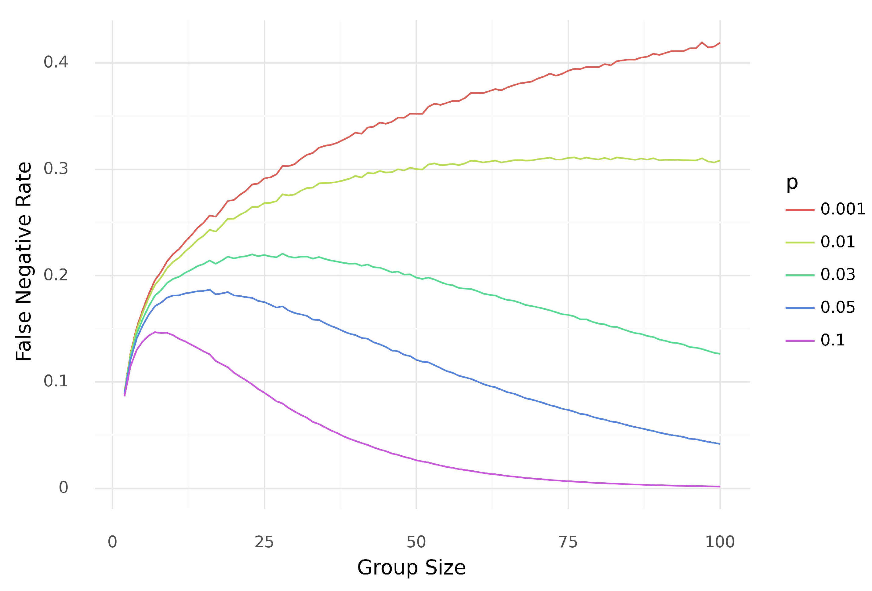
2.2.1. Estimation of the False Negative Rate

A censored model was proposed for FNR [12]. If the viral load of a sample is larger than LoD, the FNR will be negligible. However, when the viral load is less than LoD, the FNR of this difficult sample will be estimated. A logistic curve was proposed to fit the relationship between the FNR and C t values [13]. The new logistic regression model recognizes that FNR will strictly increase as the C t value becomes larger. The FNR model is:
FNR ( C t ) = 1 1 + exp ( 12.5 ( C t 35.8 ) ) .
The location parameter, 35.8 , and scale parameter, 12.5 , were estimated to make FNR ( C t ) meet the following two properties:
  • FNR ( d cens ) = 0.05
  • E ( FNR ( C t ) | C t > d cens ) = β , where β = 0.8

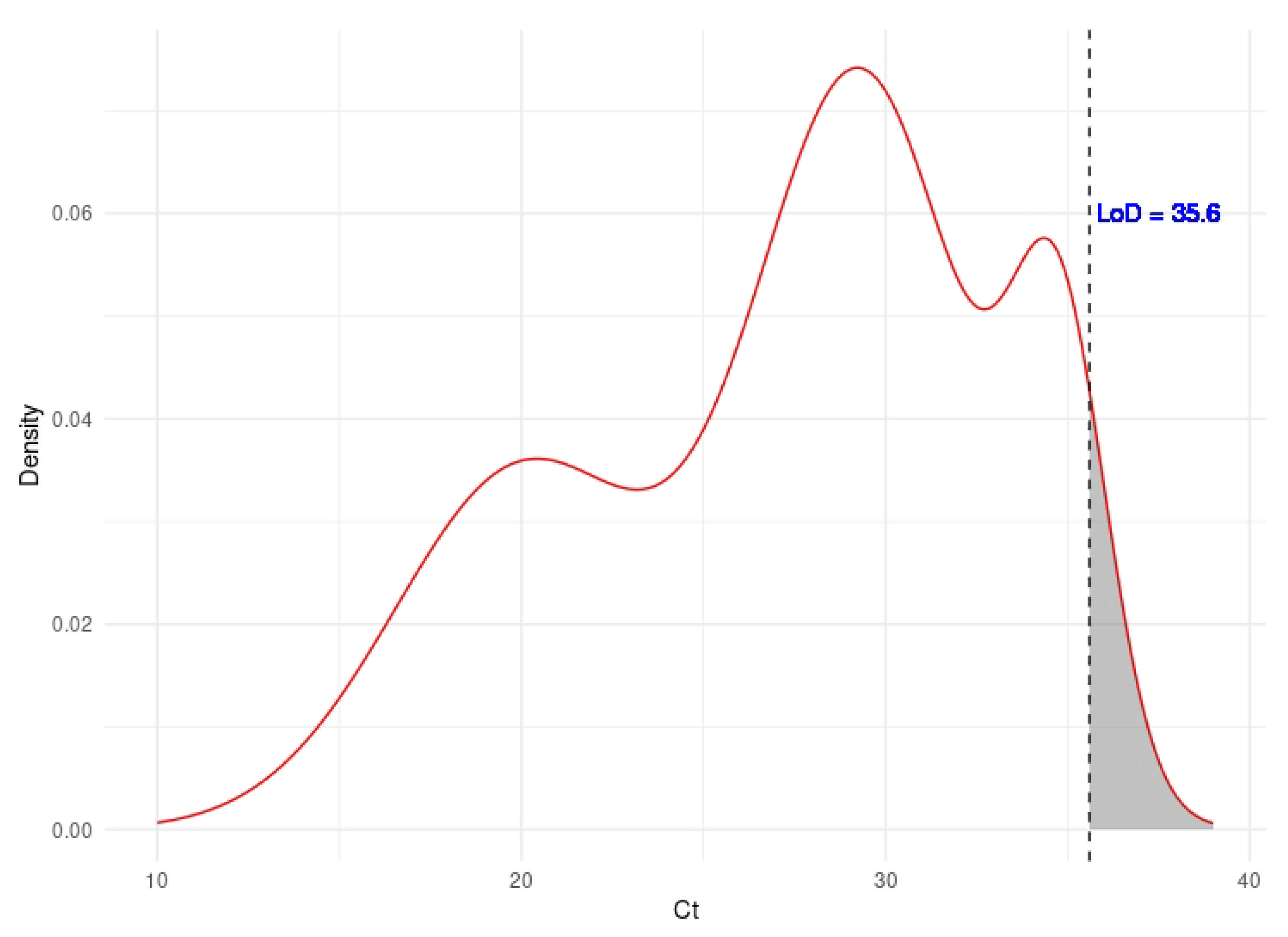
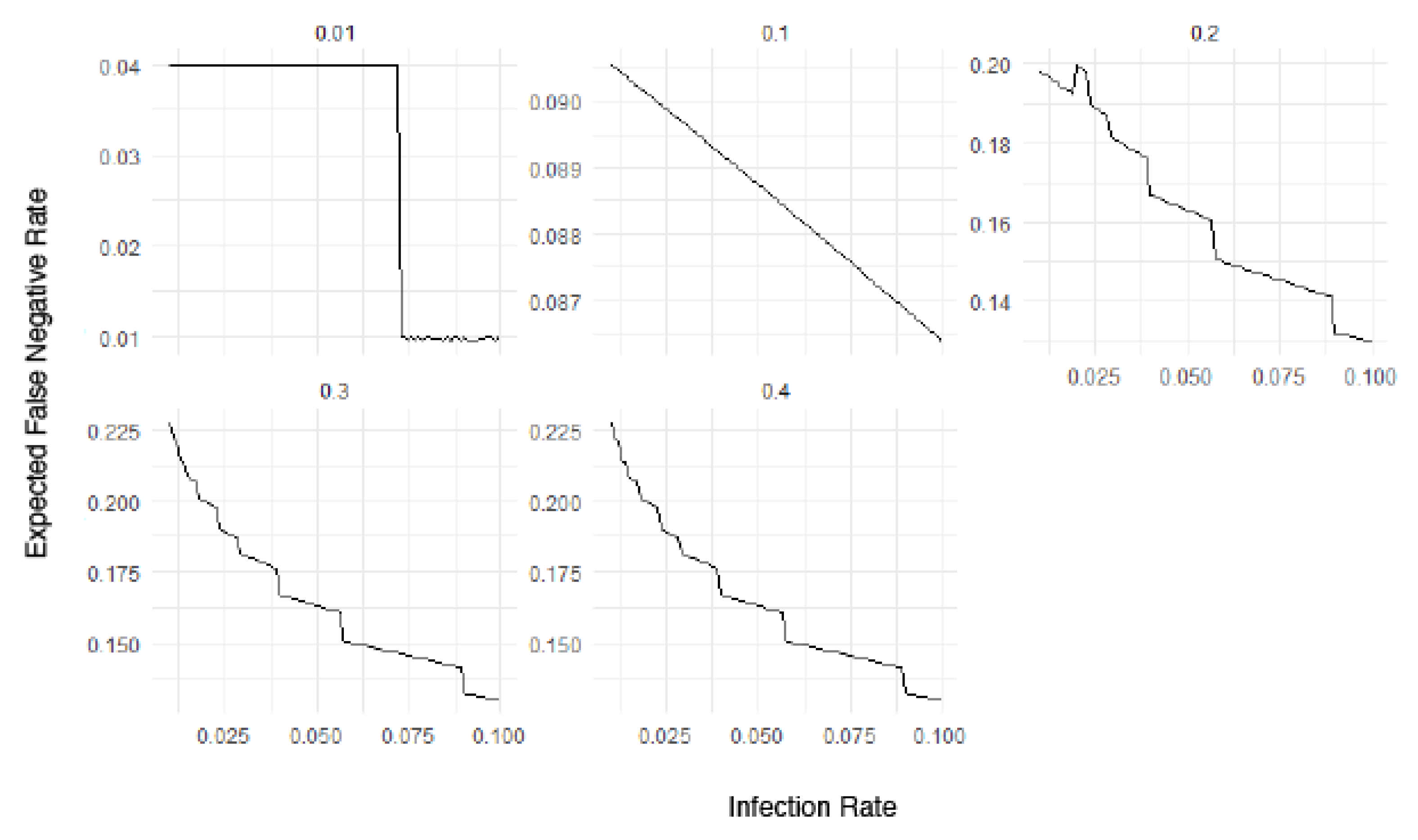
2.2.2. Dilution Effect Functions

Optimal pool sizes were derived for Dofman’s procedure when pooled testing is subject to dilution effects [7]. Given the pool size n and the number of positive cases d, he proposed that the group sensitivity function for d 1 is:
S eG ( n , k ) = p 1 ( 1 p ) n k 1 ,
where k is a dilution parameter such that 0 k 1 . No dilution effect corresponds to k = 0 . When k = 1 , the group-testing sensitivity,
S eG ( n , 1 ) = p 1 ( 1 p ) n 1 ,
can be interpreted as the probability of a sample randomly selected from a group of size n being positive.
The concentration d / n determines the sensitivity of group testing [8]. If n is fixed, S eG ( n , d ) increases in d. The faster S eG ( n , d ) converges to the sensitivity of individual testing as d approaches n, the lower the dilution effect. Ordered pooling is shown to be the most efficient way to group patients if S eG ( · , d ) is concave [9]. This conclusion generalizes the ordered pooling algorithm of [10] from no testing error to testing error with dilution effects based on (3) and (4).
Dilution effects were modeled in a molecular level [12,13]. Based on large-scale COVID-19 clinical data sets used in [11], researchers proposed more realistic dilution models. The average viral load of a pooled sample is n 1 i = 1 d V i . By the relationship between V and C t = log 2 V , the C t , G value of the pooled sample is:
C t , G = log 2 1 n i = 1 d V i = log 2 1 n i = 1 d 2 C t , i .
The group testing FNRs were determined by (5) and (2). Monte Carlo simulations were conducted [13] to estimate the expected FNR for a pooled sample given n and d. We follow the notation of [13], and let γ ( n , d ) denote the expected FNR.
In practice, we do not know d before testing. In contrast, the infection rate of a population is usually roughly estimated by a specific group testing. Inspired by γ ( n , d ) , we propose the expected FNR:
β ( n , p ) = d = 1 n γ ( n , d ) n d p d ( 1 p ) n d 1 ( 1 p ) n
for n and the infection rate of the population p. Figure 2 shows the expected FNR versus the pool size under different infection rates. For low infection rates, such as 0.001 and 0.01 , the associated FNR becomes higher when the pool size increases. In contrast, for higher infection rates, the associated FNR becomes lower when the pool size becomes larger. The reason behind this phenomenon is concentration. Under the environment of a low infection rate, the viral concentration becomes lower if we increase the group size. However, the viral concentration will become dense if we increase the group size when the infection rate is high.

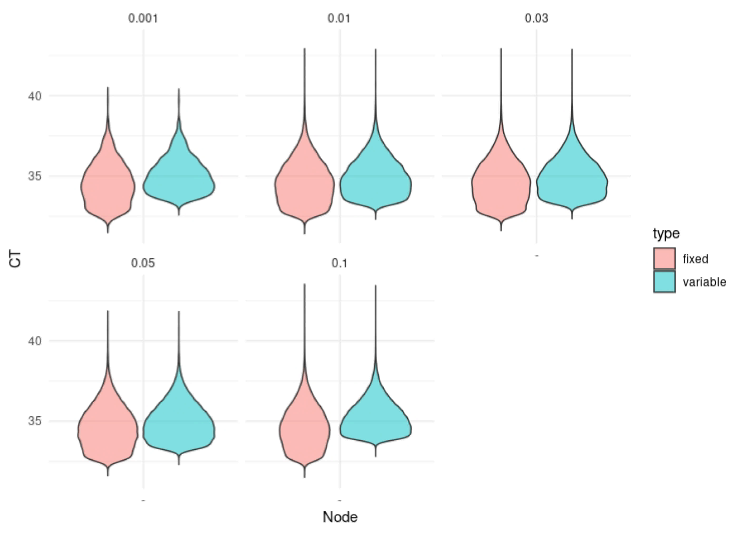
2.3. Multi-Step Group Testing with Dilution Effects

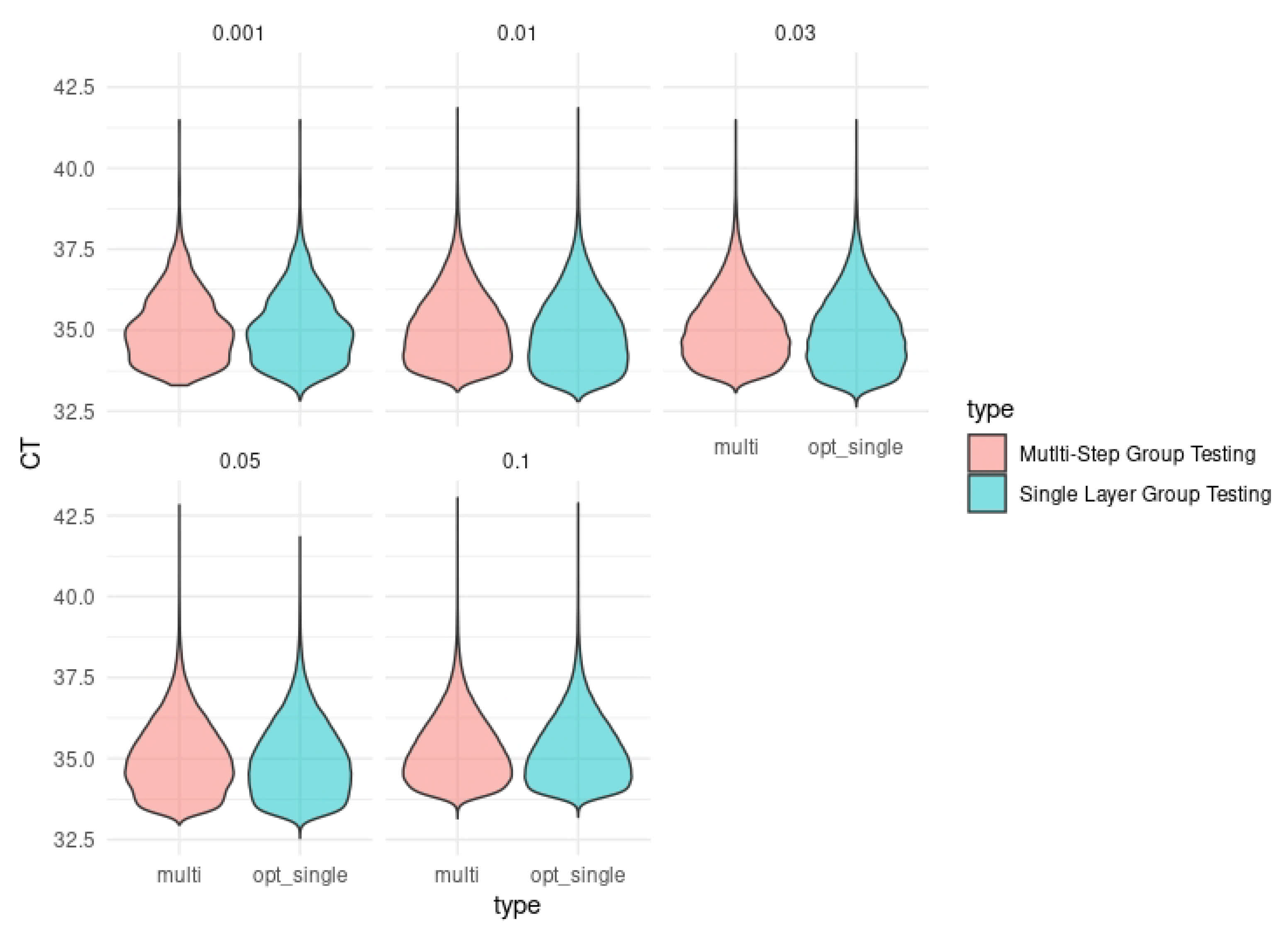
2.3.1. Multi-Step Group Testing

Multi-step group testing followed by sequential tests achieved high efficiency and efficacy when the dilution effect is not included in the model [5]. Group tests are repeated until the process results in three batch negatives or three batch positives. Each round of the multi-step group testing will depend on the previous group testing results. Negative sub-populations can be retested with a larger group size since the probability of for positive incidents is substantially reduced. Meanwhile, a positive sub-population tends to use groups with smaller sizes for retesting due to the increased probability of positives. The group size of the next iteration is determined by the optimizing the expected number of tests. After several rounds, the majority of the population will not need further investigations while others with 3 positive group test results will need individual tests. We noticed that some of the very large optimal group sizes are impractical. Some frequent group negatives such as or + can yield an optimal group size over 1000 in a later stage when the infection rate is as low as 0.1 % . Figure 3 compares test consumption of multi-step group testing with different group size upper limits. Group size upper limits have effects on the number of group tests when the population infection rate is low. The multi-step group testing procedure is more robust in sensitivity when a group size upper limit is implemented.

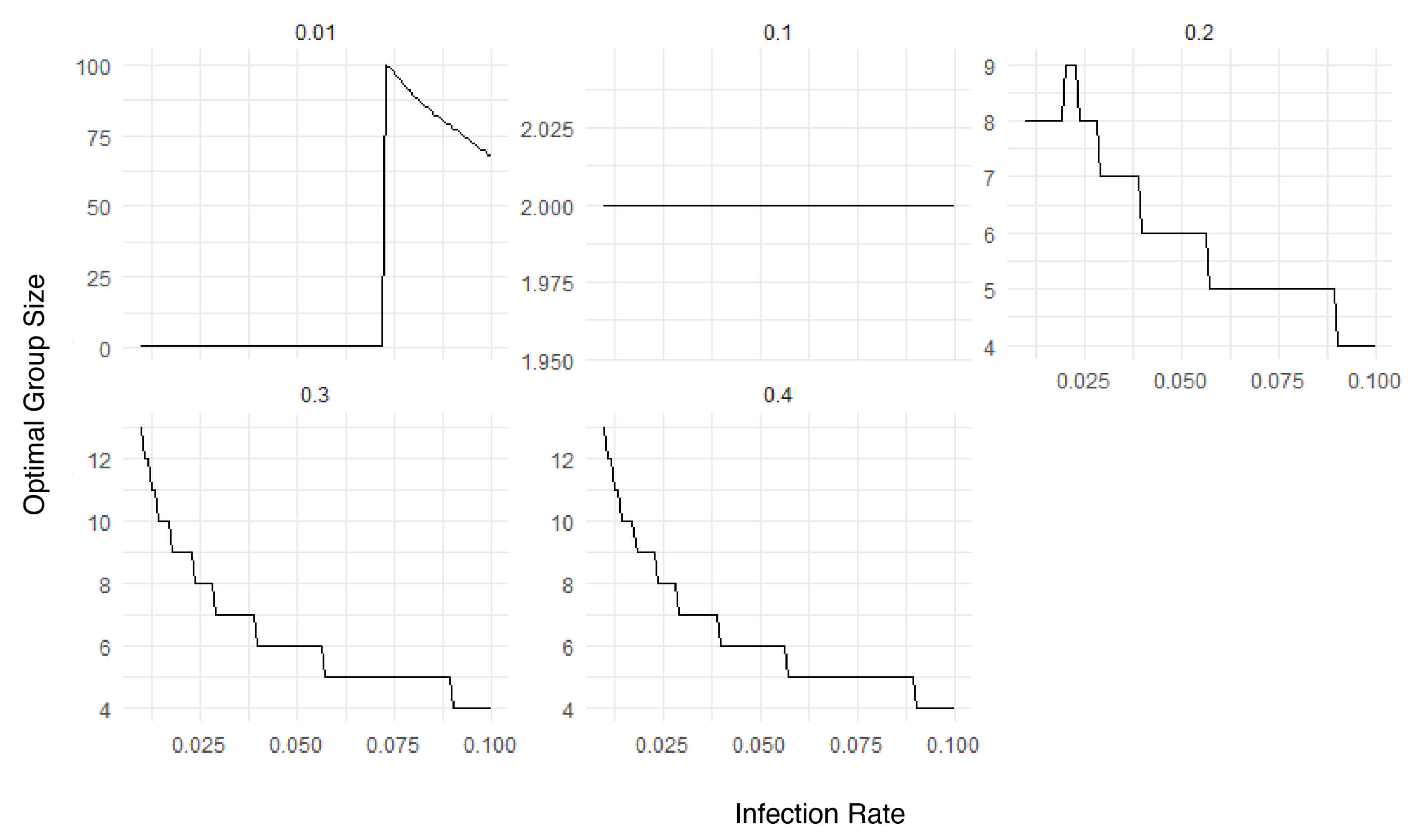
2.3.2. Optimal Group Size
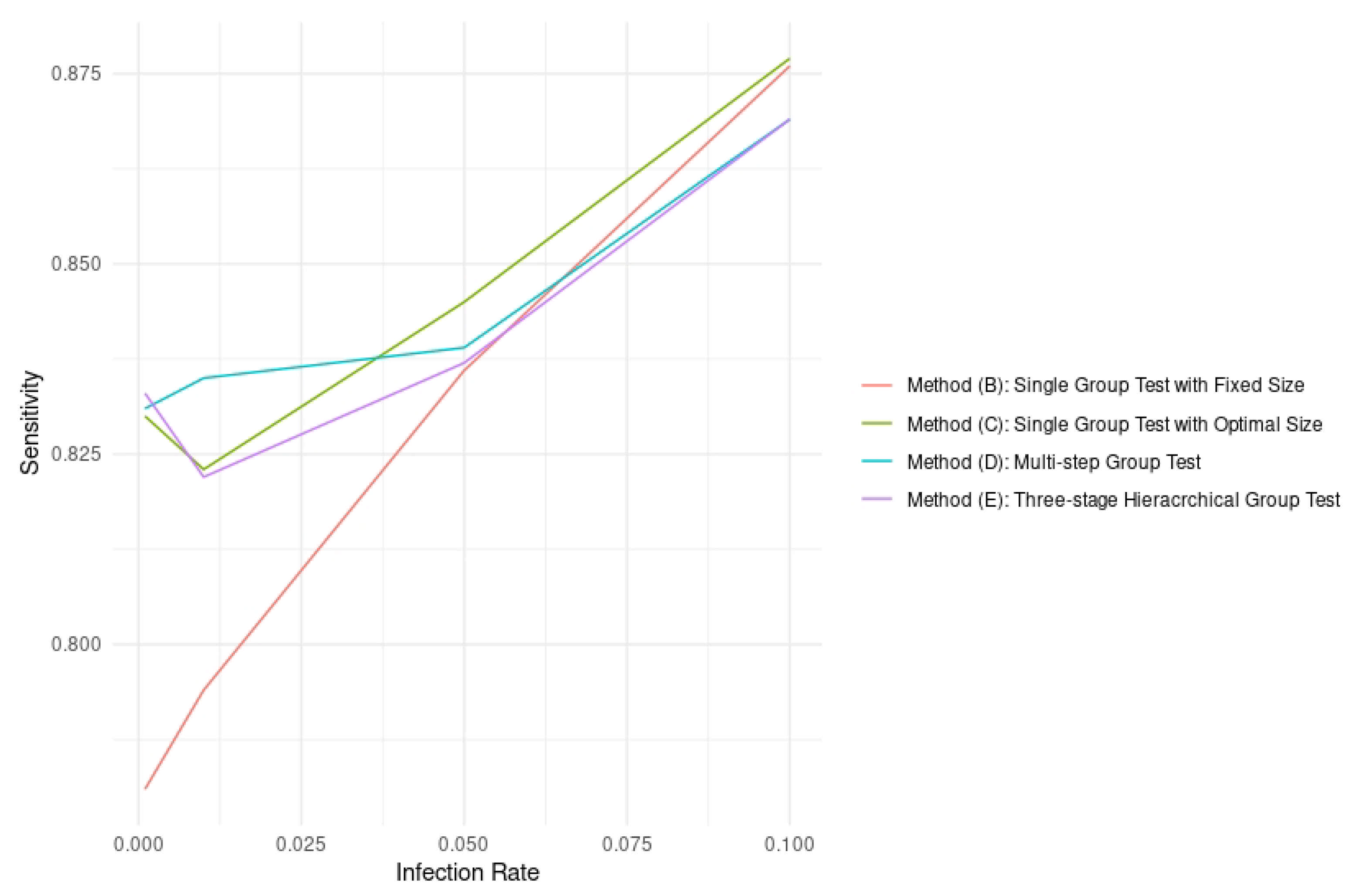
The size of a group determines the efficiency of group testing. Laboratories are interested in minimizing the required number of tests. Traditionally, research on group testing has focused solely on the expected number of tests per individual [1,4]. Given the probability of a type I error and the probability of a type II error, the expected number of tests per person without dilution setting, T ( n ) , is:
T ( n ) = 1 n + 1 Pr ( Type II Error ) [ 1 Pr ( Type I Error ) Pr ( Type II Error ) ] ( 1 p ) n .
The accuracy, sensitivity, and other measures were considered by [5], as well as the number of tests, and [15] included the expected number of tests and accuracy. Both the costs of collecting the samples and those of running the assays were considered by [16]. An extension of the objective function was discussed to array testing over a number of realistic situations [17]. They showed that controversy between different objective functions may be useless since the corresponding results are largely the same for standard testing algorithms in a wide variety of situations.
Before we derive the expected number of tests per person based on (7) for Dorman’s method, we first show the probability in each cell of the confusion matrix for group testing results for the infection rate p. Table 1 shows the probabilities for the confusion matrix, where γ ( n , 0 ) denotes the probability that a group of size n with no positive cases test negative.
Test result + needs n + 1 tests, whereas test result − needs only one test. The expected number of tests per person under the dilution setting, T ( n ) , is:
T ( n ) = ( ( 1 p ) n γ ( n , 0 ) + d = 1 n p d ( 1 p ) n d γ ( n , d ) ) × 1 n + d = 1 n n d p d ( 1 p ) n d ( 1 γ ( n , d ) + ( 1 γ ( n , 0 ) ) ( 1 p ) n ) ( 1 n + 1 ) = ( 1 p ) n 1 γ ( n , 0 ) + 1 n + d = 1 n 1 + 1 n γ ( n , d ) n d p 1 p d .
A selection of the group size is an optimization problem. We seek to minimize T ( n ) subject to the expected FNR β ( n , p ) given in (6) not exceeding a given level C. The optimization problem can be written as:
min n { 1 , 2 , , n max } T ( n ) such that β ( n , p ) C ,
where n max is the upper limit of the group size.
Figure 4 shows the optimal group size among different infection rates with different thresholds for the expected FNR β ( n , p ) . Figure 5 illustrates the expected FNR given the optimal group size under the different thresholds. A group of size 1 is returned for a threshold of 0.01 because even the individual testing cannot achieve the threshold of FNR. Except for low thresholds of 0.01 and 0.1, we can notice that the optimal group size gradually decreases as the infection rate increases. As a result, the viral concentration in pooling increases with an optimal size. The expected FNR given the optimal group size tends to decrease gradually when the infection rate increases as well.

2.3.3. Sensitivity

The sensitivity of Dorfman’s method is ( 1 β ) 2 under no dilution effect assumption [4,5,18]. Note that it does not depend on n or d. We can extend this result by taking into account the dilution effect. To identify an infection as test positive, we want to make no error on neither the pooled testing nor the individual testing. Given the infection rate p, the probability of making no error on pooled testing is 1 β ( n , p ) . It is intractable to estimate the probability that an individual received a correct test result. The reason is because the pooling result depends on other samples in the same group. If an infected sample has very low viral load and it happens to be in the same group as other infected samples with high viral load, it is possible that individual testing fails to detect the samples with low viral loads. If we ignore those complicated hierarchical relations, we can assume that the individual test result is independent to the pooled test result. Then, the approximate sensitivity, given p and n, is:
( 1 β ( n , p ) ) ( 1 γ ( 1 , 1 ) ) .
Table 2 shows a comparison between the approximate sensitivity based on (10) and the simulated sensitivity for a fixed group size of 10 and different infection rates. The population size is 100,000 with 100 repetitions.
Multi-step group testing methods [5] mitigate the false negative issue without considering dilution effects. Every sample was taken with a few rounds of pooled testing and possible individual tests. At the end of each round, samples in a negative sub-population entered into a larger group in the next round. There is one caveat for multi-step group testing under the assumption of dilution effects. If there are infected samples in a negative sub-population, we will pool those false negative cases in the group with a larger size. The infection rate in the larger pooling size will be lower. We use Figure 2 as an example. If the infection rate of the whole population is 0.03 and the group size is 25, then the expected FNR is around 0.22 . After the first round of group testing, we can obtain negative sub-populations and positive sub-populations. Among the negative sub-populations, there can be false negative cases, and the infection rate is lower than 0.03 . Multi-step group testing moves the samples in a negative sub-population into a larger group. For example, if the infection rate of the negative sub-population is 0.01 and the group size is 50, the expected FNR will become higher than 0.3 .
Dilution effects make further rounds of group testing on negative sub-populations even harder. Hence, we propose in this study that all the groups in the negative sub-populations are tested twice in each round of the multi-step group testing to reduce FNR caused by dilution effects. Samples in the negative groups in the second test will be advanced to the negative sub-population for the next round. The samples in the positive group in the second test will be advanced to the positive sub-population in the next round. Figure 6 shows the negative repetition. For a negative repetition in round k, the expected reduction of the number of false negatives is n p ( β ( n , p ) β ( n , p ) k + 1 ) , and it is k 1 n p ( β ( n , p ) β ( n , p ) k + 1 ) per test kit. This number decreases as k increases, and therefore, it is not efficient to conduct further testing for the cases from the negative repetition.

3. Results

We conducted a Monte Carlo simulation study to evaluate the efficiency and efficacy of group testing procedures in the dilution effects setting. The simulation results are given in Table 3. A population of 100,000 people is randomly generated 100 times. The infection rates of 0.1 % , 1 % , 3 % , 5 % , and 10 % are chosen. For the infected people, C t follows (1). The FNR function given C t is given in (2). We compared the classification metrics for (A) individual tests; (B) single group testing with a fixed size 10; (C) single group testing with optimal group sizes; (D) multi-step group tests ending with two batch negatives or two batch positives, with an individual test given to two batch positives; and (E) three stage hierarchical group testing, which will divide positive groups into smaller, non-overlapping subgroups twice until all positive specimens are confirmed by individual testing. For (C), (D), and (E), the group size is determined by (9) for the sub-populations in each step. For each of the infection rates, the overall accuracy, sensitivity, specificity, PPV (positive predictive value: proportion of true positives among test positives), and NPV (negative predictive value: proportion of true negatives among test negatives) are obtained, and the required number of tests to cover the whole population is calculated. The values are averaged over the 100 repetitions.
Conventional individual testing performs better in accuracy and sensitivity than any group testing methods. The sensitivity of individual testing is around 0.95 due to the probability that an infected person has C t , which is beyond the detection limit of around 5 % . The C t value of the pool will be high and beyond LoD, even when we use the optimal group size and the infection rate is low.
The sensitivity of group testing method is found to be equal in different infection rates when there are no dilution effects [5]. However, with dilution effects and FNR functions of C t , the sensitivity of the group testing methods increases if the infection rate goes up. It is because a higher infection rate raises the viral load concentration in a pooling sample and therefore reduces FNR. Figure 7 shows that the simulated sensitivity of (B), (C), (D), and (E) increased as the infection rate increased.
Method (C) improved the sensitivity by using optimal group sizes instead of a fixed group size in method (B). Figure 8 shows the C t value distribution in the negative sub-population for a fixed group size (method (B)) and the optimal group size (method (C)). The C t distribution for C t > 35.6 is almost identical for methods (B) and (C). However, the distribution of C t is lower in (B) than in (C) for C t < 35.6 . Method (C) made less false negatives for the samples with low C t . For the infection rates of 0.001 and 0.01 , the number of tests for method (C) was larger than that of method (B). However, when the infection rate became larger than 1 % , the number of tests in method (C) started to be less than that of method (B).
Method (D) improved the sensitivity by multi-step group testing over single layer group testing in method (C) for infection rates of 0.001 and 0.01 . Figure 9 shows the distribution of C t in the negative sub-populations for method (C) and method (D). The comparison of the distributions of C t between method (C) and method (D) was identical to the comparison between method (B) and method (C). Method (D) yielded less false negatives for samples with low C t values. The violin plot shapes of methods (C) and (D) for the low C t values are slightly different for an infection rate of 0.001 . For the infection rates of 0.05 and 0.1 , the C t distributions for methods (C) and (D) were almost identical, but the difference in sensitivity was 0.006 and 0.007 between multi-step group testing and single layer group testing for infection rates of 0.05 and 0.1 , respectively.
Method (D) improved over Method (C) for certain infection rates. Table 4 shows the changes in false negatives between step I and step II of multi-step group testing. The multi-step architecture could not reduce false negatives by increasing steps when the dilution effect was assumed in this study. The reason is because the previous false negatives fell into groups with larger sizes, yielding even higher dilution effects.
Method (E) can be considered the variation of method (D), which does not advance to further tests on negative sub-populations. Three-stage hierarchical group tests could not improve the sensitivity compared to the Dorfman group testing but improved the test efficiency. Our simulations showed that the difference in sensitivity between method (E) and method (C) was less than 1 % . Method (E) saved 7 % of test consumption compared to method (C) for the infection rate of 5 % .

4. Discussion

Some infectious diseases spread silently by asymptomatic carriers, and we need a rapid testing of the virus for all the residents of each community. It requires more efficient testing methods than individual testing. Group testing is a natural candidate.
Compared to individual testing, group testing increases FNR. In this study, we have a comprehensive discussion of dilution effects, one major concern for the implementation of the group testing. The pooling result depends on other samples in the same group. This is a limitation of the pooled tests. If we ignore those complicated hierarchical relations, we can assume that the individual test result is independent to the pooled test result. Using over 3000 samples, we modeled the dilution effects. Furthermore, under this specific dilution effect, we can estimate the optimal group size via Monte Carlo simulation. The optimal group size is determined by the infection rate and the dilution effect. Single group testing with an optimal size performs better on both sensitivity and test efficiency than single group testing with a fixed size of 10. The group size of 10 is widely used for COVID-19 group testing.
Based on our simulation study, we recommend single group testing with optimal group sizes. Multi-step group testing cannot improve the sensitivity from single group testing with an optimal size due to the dilution effect. The reason for this is because the samples with false negatives in the previous group are pooled into a larger group, causing a larger dilution effect. More people in the community can be covered by improving the efficiency of tests. Multi-stage hierarchical group testing, a variation of multi-step group testing, can improve the efficiency of testing by a reduction in test consumption when it has less than 1 % in sensitivity comparing to the single-layer group testing with optimal group size.
Our dilution effect modeling and simulation tool will be useful to determine an optimal group test. It can be easily applied to various infectious diseases. For COVID-19, for example, the presence of the viral load in the patients can vary over more than nine orders of magnitude [19]. Therefore, any lab using group testing needs a simulation tool to monitor/optimize its group testing regularly. In future studies, we will continue investigating the dilution effect to improve test efficiency and efficacy. Other group testing methods such as overlapping group tests will be investigated as well.

Author Contributions

H.J., H.A. and X.L. designed the model; H.J. performed the simulation; H.J. and H.A. analyzed the simulation data; H.J. and H.A. wrote the paper; X.L. reviewed, edited the manuscript; X.L. and H.A. acquired funding. All authors have read and agreed to the published version of the manuscript.

Funding

Xiaolin Li and Haoran Jiang are supported in part by the US Army Research Office grant W911NF18-10346. Xiaolin Li and Hongshik Ahn are supported in part by the US Army Research Office equipment grant W911NF-20-10159.

Data Availability Statement

The main Python simulation code was posted at https://github.com/Haoran-Jiang/group_testing_with_dilution (accessed on 28 December 2021). Please contact Haoran Jiang, haoran.jiang@stonybrook.edu for further information.

Conflicts of Interest

The authors declare no conflict of interest.

Abbreviations

The following abbreviations are used in this manuscript:
PCRPolymerase chain reaction
RT-PCRReverse transcription-Polymerase chain reaction
FNRFalse negative rate

References

  1. Dorfman, R. The detection of defective members of large populations. Ann. Math. Stat. 1943, 14, 436–440. [Google Scholar] [CrossRef]
  2. Hogan, C.A.; Sahoo, M.K.; Pinsky, B.A. Sample pooling as a strategy to detect community transmission of SARS-CoV-2. JAMA 2020, 323, 1967–1969. [Google Scholar] [CrossRef] [PubMed] [Green Version]
  3. Abdalhamid, B.; Bilder, C.R.; McCutchen, E.L.; Hinrichs, S.H.; Koepsell, S.A.; Iwen, P.C. Assessment of specimen pooling to conserve SARS CoV-2 testing resources. Am. J. Clin. Pathol. 2020, 153, 715–718. [Google Scholar] [CrossRef] [PubMed] [Green Version]
  4. Kim, H.; Hudgens, M.G.; Dreyfuss, J.M.; Westreich, D.J.; Pilcher, C.D. Comparison of group testing algorithms for case identification in the presence of test error. Biometrics 2007, 63, 1152–1163. [Google Scholar] [CrossRef] [PubMed]
  5. Ahn, H.; Jiang, H.; Li, X. Modeling and computation of multistep batch testing for infectious diseases. Biom. J. 2021, 63, 1272–1289. [Google Scholar] [CrossRef] [PubMed]
  6. Bilder, C.R.; Iwen, P.C.; Abdalhamid, B.; Tebbs, J.M.; McMahan, C.S. Tests in short supply? Try group testing. Significance 2020, 17, 15–16. [Google Scholar] [CrossRef] [PubMed]
  7. Hwang, F.K. Group testing with a dilution effect. Biometrika 1976, 63, 671–673. [Google Scholar] [CrossRef]
  8. Burns, K.C.; Mauro, C.A. Group testing with test error as a function of concentration. Commun. Stat.-Theory Methods 1987, 16, 2821–2837. [Google Scholar] [CrossRef]
  9. Saraiva, G. Pool testing with dilution and heterogeneous priors. Preprint. 2021. Available online: https://papers.ssrn.com/sol3/papers.cfm?abstract_id=3789077 (accessed on 28 December 2021).
  10. Hwang, F.K. A generalized binomial group testing problem. J. Am. Stat. Assoc. 1975, 70, 923–926. [Google Scholar] [CrossRef]
  11. Jones, T.C.; Biele, G.; Mühlemann, B.; Veith, T.; Schneider, J.; Beheim-Schwarzbach, J.; Bleicker, T.; Tesch, J.; Schmidt, M.L.; Sander, L.E.; et al. Estimating infectiousness throughout SARS-CoV-2 infection course. Science 2021, 373. [Google Scholar] [CrossRef] [PubMed]
  12. Brault, V.; Mallein, B.; Rupprecht, J. Group testing as a strategy for COVID-19 epidemiological monitoring and community surveillance. PLoS Comput. Biol. 2021, 17, e1008726. [Google Scholar] [CrossRef] [PubMed]
  13. Lin, Y.; Ren, Y.; Wan, J.; Cashore, M.; Wan, J.; Zhang, Y.; Frazier, P.; Zhou, E. Group testing enables asymptomatic screening for COVID-19 mitigation: Feasibility and optimal pool size selection with dilution effects. arXiv 2020, arXiv:2008.06642. [Google Scholar]
  14. Yelin, I.; Aharony, N.; Tamar, E.; Argoetti, A.; Messer, E.; Berenbaum, D.; Shafran, E.; Kuzli, A.; Gandali, N.; Shkedi, O.; et al. Evaluation of COVID-19 RT-qPCR test in multi sample pools. Clin. Infect. Dis. 2020, 71, 2073–2078. [Google Scholar] [CrossRef] [PubMed]
  15. Malinovsky, Y.; Albert, P.S.; Roy, A. Reader reaction: A note on the evaluation of group testing algorithms in the presence of misclassification. Biometrics 2016, 72, 299–302. [Google Scholar] [CrossRef] [PubMed]
  16. Huang, S.; Huang, M.L.; Shedden, K. Cost considerations for efficient group testing studies. Statstica Sin. 2020, 30, 285–302. [Google Scholar] [CrossRef]
  17. Hitt, B.D.; Bilder, C.R.; Tebbs, J.M.; McMahan, C.S. The objective function controversy for group testing: Much ado about nothing? Stat. Med. 2019, 38, 4912–4923. [Google Scholar] [CrossRef] [PubMed]
  18. Johnson, N.L.; Kotz, S.; Wu, X. Inspection Errors for Attributes in Quality Control; CRC Press: New York, NY, USA, 2020. [Google Scholar]
  19. Batson, J.; Bottman, N.; Cooper, Y.; Janda, F. A comparison of group testing architectures for COVID-19 testing. arXiv 2020, arXiv:2005.03051. [Google Scholar]
Figure 1. C t distribution among positive cases.
Mathematics 10 00497 g001
Figure 2. Expected FNR vs. pool size under different infection rates.
Mathematics 10 00497 g002
Figure 3. Number of tests for multi-step group testing for population size 100,000 with three different group size upper limits: 32, 64, and 10,000.
Mathematics 10 00497 g003
Figure 4. Optimal group size for different infection rates with different expected FNR thresholds. The infection rate ranges from 0.001 to 0.1; expected FNR thresholds are 0.01, 0.1, 0.2, 0.3, and 0.4.
Mathematics 10 00497 g004
Figure 5. Expected FNR given optimal group size under different thresholds. The infection rate ranges from 0.001 to 0.1; the expected FNR thresholds are 0.01, 0.1, 0.2, 0.3, and 0.4.
Mathematics 10 00497 g005
Figure 6. Negative sub-population in a repeated testing procedure.
Mathematics 10 00497 g006
Figure 7. Sensitivity of group tests as the infection rate varies. Generally, the sensitivity of group test methods increases as the infection rate increases.
Mathematics 10 00497 g007
Figure 8. False negative C t values of single layer group testing with fixed group size and optimal group size for each of the infection rates: 0.001, 0.01, 0.03, 0.05, and 0.1.
Mathematics 10 00497 g008
Figure 9. False negative C t values of multi-step group testing and single layer group testing for each of the infection rates: 0.001, 0.01, 0.03, 0.05, and 0.1.
Mathematics 10 00497 g009
Table 1. Probabilities for the confusion matrix for group testing results.
True Condition
No Samples Are InfectedAt Least One Sample is Infected
Test+ ( 1 γ ( n , 0 ) ) ( 1 p ) n d = 1 n ( 1 γ ( n , d ) ) n d p d ( 1 p ) n d
Result γ ( n , 0 ) ( 1 p ) n d = 1 n γ ( n , d ) n d p d ( 1 p ) n d
Table 2. Approximate sensitivity vs. simulated sensitivity given pool size 10, population size 100,000, and 100 repetitions.
pGroup SizeApproximate SensitivitySimulated Sensitivitysd
0.001 10 0.7798 0.7824 0.0364
0.01 10 0.7871 0.7919 0.0124
0.03 10 0.8031 0.8156 0.0076
0.05 10 0.8188 0.8357 0.0054
0.1 10 0.8561 0.8770 0.0037
Table 3. Simulation results: 100 repetitions, population size 100,000; mean with standard deviation in parentheses.
p ( 1 ) 0.0010.010.030.050.10
(A) a Acc. ( 2 ) 0.999 (0.000)0.999 (0.000)0.998 (0.000)0.997 (0.000)0.995 (0.000)
IndivSens. ( 3 ) 0.955 (0.018)0.960 (0.005)0.960 (0.005)0.960 (0.000)0.959 (0.000)
TestsSpec. ( 4 ) 10.000 (0.000)10.000 (0.000)10.000 (0.000)0.998 (0.000)0.995 (0.000)
PPV0.484 (0.020)0.910 (0.010)0.968 (0.002)0.983 (0.002)0.990 (0.001)
NPV10.000 (0.000)10.000 (0.000)0.999 (0.000)0.998 (0.000)0.995 (0.000)
#Tests ( 5 ) 100,000 (0)100,000 (0)100,000 (0)100,000 (0)100,000 (0)
(B) b Acc.10.00 (0.000)0.998 (0.000)0.994 (0.000)0.992 (0.000)0.987 (0.000)
SingleSens.0.781 (0.042)0.794 (0.013)0.815 (0.008)0.836 (0.001)0.876 (0.000)
GroupSpec.10.000 (0.000)10.000 (0.000)10.000 (0.000)10.000 (0.000)10.000 (0.000)
TestsPPV0.990 (0.012)0.992 (0.004)0.992 (0.002)0.993 (0.001)0.995 (0.001)
FixedNPV10.00 (0.000)0.998 (0.000)0.994 (0.000)0.991 (0.000)0.986 (0.000)
Size 10#Tests10,878 (91)17,649 (261)31,190 (348)42,926 (463)65,750 (500)
(C) c Acc.10.00 (0.000)0.998 (0.000)0.995 (0.000)0.992 (0.000)0.988 (0.000)
SingleSens.0.830 (0.038)0.823 (0.013)0.834 (0.006)0.845 (0.005)0.877 (0.003)
GroupSpec.10.000 (0.000)10.000 (0.000)10.00010.000 (0.000)10.000 (0.000)
OptimalPPV0.994 (0.010)0.995 (0.002)0.995 (0.001)0.996 (0.001)0.998 (0.001)
SizesNPV10.00 (0.000)0.998 (0.000)0.995 (0.000)0.992 (0.000)0.987 (0.000)
#Tests20,517 (54)21,579 (158)30,569 (257)38,872 (352)54,995 (304)
B+Ind ( 6 ) 20,000 + 51716,667 + 49116,667 + 13,90216,667 + 22,20525,000 + 29,995
(D) d Acc.10.00 (0.000)0.998 (0.000)0.995 (0.000)0.992 (0.000)0.987 (0.000)
Multi-stepSens0.0.831 (0.039)0.835 (0.012)0.841 (0.000)0.839 (0.006)0.869 (0.004)
GroupSpec0.10.000 (0.000)10.000 (0.000)10.000 (0.000)10.000 (0.000)10.000 (0.000)
VariablePPV0.997 (0.006)0.997 (0.002)0.998 (0.001)0.998 (0.001)0.999 (0.000)
SizesNPV10.00 (0.000)0.998 (0.000)0.995 (0.000)0.992 (0.000)0.986 (0.000)
1 indiv#Tests40,388 (41)40,396 (126)46,898 (191)50,739 (280)70,175 (290)
TestB+Ind40,082 + 30637,278 + 311839,571 + 732738,801 + 11,93848,314 + 21,861
(E) eAcc.10.00 (0.000)0.998 (0.000)0.995 (0.000)0.992 (0.000)0.987 (0.000)
Three StageSens0.0.833 (0.034)0.822 (0.014)0.829 (0.007)0.837 (0.005)0.869 (0.003)
HierarchicalSpec.10.000 (0.000)10.000 (0.000)10.000 (0.000)10.00 (0.000)10.00 (0.000)
VariablePPV0.998 (0.006)0.997 (0.002)0.998 (0.001)0.998 (0.001)0.999 (0.000)
SizesNPV10.00 (0.000)0.998 (0.000)0.995 (0.000)0.991 (0.000)0.986 (0.000)
Group#Tests20,436 (48)20,964 (154)28,527 (224)35,956 (304)56,906 (295)
TestB+Ind20,130 + 30617,896 + 306721,308 + 721924,078 + 11,87835,013 + 21,893
a Conventional individual tests. b One-step batch tests with a fixed batch size of 10, individual tests for positive batches. c One-step batch tests with variable batch sizes. d Multi-step batch tests with variable optimal batch sizes; an individual test for 2 batch positives. e Three stage hierarchical group tests with variable optimal group sizes. ( 1 )  infection rate, ( 2 ) overall accuracy, ( 3 ) sensitivity, ( 4 ) specificity, ( 5 ) number of required tests, ( 6 )  number of batch tests + number of individual tests.
Table 4. Simulation results: 100 repetitions, population size 100,000; mean with standard deviation in parentheses.
pStep I False NegativesStep II False Negatives
0.00114.4 (5.86)15.3 (4.87)
0.0188.2 (74.8)86.3 (80.4)
0.03242 (203)235 (210)
0.05367 (350)392 (325)
0.1717 (546)623 (510)
Publisher’s Note: MDPI stays neutral with regard to jurisdictional claims in published maps and institutional affiliations.

