Graph Learning for Attributed Graph Clustering

Abstract

Due to the explosive growth of graph data, attributed graph clustering has received increasing attention recently. Although deep neural networks based graph clustering methods have achieved impressive performance, the huge amount of training parameters make them time-consuming and memory- intensive. Moreover, real-world graphs are often noisy or incomplete and are not optimal for the clustering task. To solve these problems, we design a graph learning framework for the attributed graph clustering task in this study. We firstly develop a shallow model for learning a fine-grained graph from smoothed data, which sufficiently exploits both node attributes and topology information. A regularizer is also designed to flexibly explore the high-order information hidden in the data. To further reduce the computation complexity, we then propose a linear method with respect to node number n, where a smaller graph is learned based on importance sampling strategy to select m$(m\ll n)$ anchors. Extensive experiments on six benchmark datasets demonstrate that our proposed methods are not only effective but also more efficient than state-of-the-art techniques. In particular, our method surpasses many recent deep learning approaches.

1. Introduction

In the era of big data, there is a great need to analyze the data that are best represented as a graph [1]. Examples include the WWW, social networks, sensor networks, biological networks, and many others [2]. Graph clustering is a crucial technique used to effectively mine and learn from such data. Its goal is to partition a graph into several disjoint communities or groups, such that each component is densely connected [3,4].

An attributed graph includes both the node content and structural relationship information [5]. For instance, in social media, such as Twitter, Weibo, and Facebook, users and their connections form a social network. The users’ personal information contains details that define their gender, place of residence, level of education, hobby, and more. It would be beneficial to group the users in a social network by taking into account both personal profiles and social relationships for user-targeted online advertising, the suggestion of services/apps, etc. [6]. Many traditional clustering techniques exploit only one of them, and thus the resultant clustering is inevitably damaged. For example, the classical k-means [7] is only applicable to feature data, while spectral clustering is a straightforward method for graph data [8]. Some algorithms have been purposely designed to handle both content and structure information, such as co-clustering technique [9], content propagation [10], and relational topic method [11]. These methods are still limited since they are directly applied on original graphs, failing to exploit the mutual corroboration effects of structures and attributes [12].

Inspired by the great success of deep learning, some auto-encoder based graph clustering methods have been proposed. For instance, the variational graph auto-encoder [13], adversarially regularized method [14], sparse auto-encoder [15], and denoising auto-encoder [2] are applied to learn deep representations for graph clustering. Despite their encouraging performance, they are restricted in some aspects. For example, the variational graph auto-encoder [13] will fail to model complex data distributions since it assumes a single Gaussian prior on the learned latent embedding. To address this limitation, the variational graph auto-encoder with Gaussian mixture model [16] has been proposed recently. To capture the different importances of the neighboring nodes to a target node, the deep attentional embedded graph clustering [17] method introduces an attention network to achieve a compact representation. However, it employs an inner product decoder to reconstruct the graph structure, which is not flexible enough to characterize various kinds of relationships in practice.

Furthermore, these deep models presume that the given graphs are optimal for downstream tasks, while real-world graphs are often noisy or incomplete [18]. Therefore, it is desired to construct a high-quality graph for these methods [19]. Besides, plenty of graph clustering methods generally build the graph for spectral clustering according to a fixed formula or hand-crafted rules, such as Euclidean distance and cosine function [20]. However, rigorously analyzing a similarity measure is still a challenge [21]. Another inherent limitation of deep models is the huge amount of training parameters, and setting the hyper-parameters requires expertise and extensive trial and error process, which makes them time-consuming and memory-intensive.

To overcome the above limitations, we propose a Graph Learning approach for Graph Clustering (GLGC) task (the code is available at https://github.com/XieXuanting/GLGC, accessed on 13 November 2022).

Different from other methods, we use smoothed features to learn an adaptive graph. This graph can also keep the initial high-order relationships. Considering that the size of it is $n\times n$ (n is the number of nodes), our method suffers from high time and space complexity. We further propose to learn a smaller graph by applying a node sampling strategy, resulting in a linear complexity with respect to n. As an extension of our previous FGC [22] method, this work addresses the scalability issue.

To sum up, the technical contributions can be classified into three types: scalable graph learning strategy, sampling method, and extensive experiments. They are elaborated as follows:

• We develop a similarity graph learning approach for graph clustering. It effectively digs the interplay between the topology and the node features. Meanwhile, it retains the initial high-order relationships;
• A node sampling strategy is applied to choose some important nodes, which makes our method scalable to a large graph;
• Extensive experimental results demonstrate the effectiveness and efficiency of our algorithm with respect to many state-of-the-art methods, including several recent deep models.

The remainder of this paper is structured as follows: in Section 2, we introduce some related methods. Then, Section 3 presents the developed method. Section 4 presents a series of experiments to validate our method. Finally, Section 5 is dedicated to the conclusion.

2. Related Work

For attributed graph clustering, it is paramount to leverage two different types of information: the graph topological structure and the node properties [23]. Generative models have been used to explore the interaction between the connectivity of graph and node attributes [24,25]. Motivated by the development of graph convolution networks (GCN), many deep graph clustering methods have been developed. To obtain a robust embedding, the adversarially regularized graph auto-encoder (ARGA) and adversarially regularized variational graph auto-encoder (ARVGA) [14], have also been developed. In particular, they build upon graph auto-encoder (GAE) and variational graph auto-encoder (VGAE) [13] to reconstruct the adjacency matrix, whose size is $n\times n$. One can clearly see that this approach will pose a great challenge for a large graph. Moreover, the above method has two steps, i.e., clustering and graph embedding are carried out in two individual stages. It is possible that the learned representations are not suitable for subsequent clustering. To address this problem, Wang et al. [17] proposed a goal-directed graph attentional auto-encoder architecture. Specifically, they employed an attention network to measure the importance of neighbors to a target node and an inner product decoder was trained to reconstruct the graph structure. Nevertheless, this approach still has a high complexity for time and space. Hui et al. [16] introduced Gaussian mixture models to VGAE to capture the inherent complex data distributions. Finally, a unified end-to-end learning model is developed for graph clustering. Wang et al. [26] introduced a neighbor-aware GAE to collect information from neighbors and use an end-to-end learning strategy. These approaches all assume that the given graphs are perfect. However, real-world graphs are often noisy or incomplete. Thus, the clustering accuracy could be compromised.

Recently, Zhang et al. [27] proposed an adaptive graph convolution (AGC) method. It uses a low-pass filter on the data to obtain a smooth representation, upon which an inner product is computed for spectral clustering. Specifically, the attribute matrix is treated as graph signals and a signal is smooth if nearby nodes have similar feature values. It was proven that smoothing a signal can remove the noise and enhance the separation of classes to some extent, thus improving the downstream task performance [28]. In other words, low-frequency basis signals dominate the high-frequency ones in a smooth graph signal [29]. Therefore, it is natural to employ a low-pass filter to obtain a clustering-friendly representation. Kang et al. [22] developed a fine-grained graph clustering (FGC) approach based on smoothed representation. Low-pass filtering based methods are simple yet effective. Unfortunately, these methods typically have a $\mathcal{O}(n^3)$ complexity and are computationally prohibitive. In this work, we extend FGC to handle a large graph by introducing a node sampling strategy. Unlike FGC, a small graph is learned for clustering.

3. Methodology

Notations: Define a non-directed graph as $\mathcal{G}=(\mathcal{V},E,X)$, where $\mathcal{V}=\{v_1,v_2,\cdots ,v_n\}$ is the set of n nodes, $X={\{x_1,\cdots ,x_n\}}^{\top }\in {\mathcal{R}}^{n\times d}$ denotes the attribute matrix, and E represents the edge set denoted by an adjacency matrix $\tilde{A}=\{{\tilde{a}}_{ij}\}\in {\mathcal{R}}^{n\times n}$. If there is an edge between $v_i$ and $v_j$, ${\tilde{a}}_{ij}=1$; otherwise, ${\tilde{a}}_{ij}=0$. With degree matrix D, symmetrically normalized adjacency matrix can be written as $A=D^{-\frac{1}{2}}(\tilde{A}+I)D^{-\frac{1}{2}}$, where a self-loop to each node is applied [3] and I is an identity matrix with a proper size. In essence, $a_{ij}$ denotes the transition probability of a single step random walk between $v_i$ and $v_j$. Then, graph Laplacian $L=I-A$. Partitioning the n nodes into g distinct groups is the goal of graph clustering.

3.1. Graph Learning

Based on the graph Laplacian manifold assumption, two similar nodes should have similar representations. Mathematically, we could achieve a smooth representation $\overline{X}$ from X by solving the following problem [30,31]:

$$\underset{\overline{X}}{min}{\parallel \overline{X}-X\parallel }_F^2+\frac{1}{2}Tr({\overline{X}}^{\top }L\overline{X}).$$

(1)

By taking the derivative of the objective function and setting it to zero, we have a closed-form solution:

$$\overline{X}={(I+\frac{L}{2})}^{-1}X.$$

(2)

However, obtaining smoothed representation in this manner is very inefficient due to the matrix inversion operation. Therefore, we approximate the inversion term by its first-order Taylor expansion, namely, $\overline{X}=(I-\frac{L}{2})X$. To aggregate information from k-th order neighbors, we then generalize it to

$$\overline{X}={(I-\frac{L}{2})}^{k}X,$$

(3)

where k controls the power of graph filtering. In practice, the raw graph is often sparse, so we define N to represent the number of nonzero elements in L. Then, we can left multiply X by $G=(I-\frac{L}{2})$ for k times, resulting in $\mathcal{O}(Ndk)$.

For clustering, it is reasonable to assume that nearby nodes are more likely to lie in the same group. Therefore, we proceed with $\overline{X}$ to enjoy the advantage of smooth representation. For notation convenience, we redefine $\overline{X}={\overline{X}}^{\top }$ in the rest of the paper. In this work, we employ the self-expression property of data to learn the relations between nodes. Specifically, it can be formulated as:

$$\underset{Z}{min}{\parallel \overline{X}-\overline{X}Z\parallel }_F^2+\alpha \mathsf{\Theta }(Z),$$

(4)

where $\alpha >0$ is a trade-off parameter. The first term evaluates the self-reconstruction quality and the second term is a regularizer. The coefficient matrix $Z\in {\mathcal{R}}^{n\times n}$ represents the relationships between nodes. In the literature, some well-known $\mathsf{\Theta }$ functions are used, such as the nuclear norm, sparse $L_1$ norm [32], and Frobenius norm [33].

As a matter of fact, real data often display structures beyond simply being low-rank or sparse. Currently, the raw affinity matrix A is not fully exploited, which is only implicitly used in graph filtering. In practice, a graph is often sparse, i.e., $\mathcal{O}(E)=\mathcal{O}(\mathcal{V})$. Thus A is incapable of modeling complex relationships among vertexes. High-order relations have been shown to be beneficial in some cases [34]. For example, the likelihood of a two-step random walk between vertices $v_i$ and $v_j$ is manifested by their second-order closeness. It is straightforward to see that the probability will be high if two nodes share many common neighbors. Similarly, P-order proximity represents the probability that a random walk starts from $v_i$ and reaches $v_j$ in P steps [35].

To benefit from the complementary information provided by different orders, we define $f(A)=A+A^2+\cdots +A^P$. Thus it is flexible to encode different orders of information by taking different P values. To incorporate $f(A)$, we design a new regularizer by requiring that the learned Z should not be too far from the original relationships characterized by $f(A)$. Then, (4) becomes

$$\underset{Z}{min}\parallel \overline{X}-\overline{X}{Z\parallel }_F^2+\alpha {\parallel Z-f(A)\parallel }_F^2.$$

(5)

We can get Z from (5) by setting its first-order derivative to zero, which gives rise to the equation:

$$Z={(\overline{X}{\overline{X}}^{\top }+\alpha I)}^{-1}(\alpha f(A)+\overline{X}{\overline{X}}^{\top }).$$

(6)

After obtaining Z, spectral clustering can be used to achieve final partitions. This is the previous FGC [22] method. However, FGC requires a lot of space and time. First, the size of Z is $n\times n$, which poses a challenge for memory. Second, the complexity for solving Z and spectral clustering is $\mathcal{O}(n^3)$. Therefore, we propose a more efficient way in the following Section.

3.2. Scalable Graph Learning

Anchor is a popular terminology in computer vision and pattern recognition [36]. Basically, it refers to a few sample items. [37]. Inspired by this, instead of using all samples to reconstruct $\overline{X}$ in (5), we can choose a subset of $m(m\ll n)$ vertexes, i.e., nodes that are significant, whose features construct $B=[b_1,\cdots ,b_m]\in {\mathcal{R}}^{d\times m}$. In other words, B is a subset of $\overline{X}$. In response, we learn a more compact graph $S\in {\mathcal{R}}^{m\times n}$, which illustrates the relations between m anchors and n nodes. Existing approaches to choose anchors are either k-means or random sampling, which fails to consider the importance of nodes. We will introduce the method for anchor selection in the next Section. According to the indexes of anchors, we can extract the complex structure relationships between all nodes and anchors from $f(A)$, which is denoted by $C\in {\mathcal{R}}^{m\times n}$. Eventually, our proposed GLAC can be formulated as:

$$\underset{S}{min}\parallel \overline{X}{-BS\parallel }_F^2+\alpha {\parallel S-C\parallel }_F^2,$$

(7)

where $\alpha$ balances the importance between structural and attribute information. The problem (7) can be easily solved by setting its first-order derivative w.r.t. S to zero, which yields

$$S={(B^{\top }B+\alpha I)}^{-1}(\alpha C+B^{\top }\overline{X}).$$

(8)

It can be seen that the inversion has a complexity of $\mathcal{O}(m^3)$ and other matrix operations take $\mathcal{O}(m^2(n+d+1)+mn(d+1))$. Thus, it is linear with respect to the amount of nodes n.

Based on S, we can obtain the affinity matrix by $S^{\top }S$ and proceed with spectral clustering, which is still computationally expensive. Therefore, we adopt a different approach.

Firstly, we normalize S by setting $\widehat{S}=H^{-1/2}S$, where H is the row sum of S. We define the singular value decomposition (SVD) of $\widehat{S}$ as $U\mathsf{\Sigma }{V}^{\top }$, where $\mathsf{\Sigma }=diag({\sigma }_1,\cdots ,{\sigma }_m)$ and $0\le {\sigma }_m\le \cdots \le {\sigma }_2\le {\sigma }_1$ are the singular values, $U=[u_1,\cdots ,u_m]\in {\mathcal{R}}^{m\times m}$ and $V=[v_1,\cdots ,v_m]\in {\mathcal{R}}^{n\times m}$ are the left and right singular vectors. It is obvious that V are also the eigenvectors of W, U are the eigenvectors of matrix $\widehat{S}{\widehat{S}}^{\top }$, and ${\sigma }_i^2$ are the eigenvalues [37]. Thus, we can calculate U based on $\widehat{S}{\widehat{S}}^{\top }$ with $\mathcal{O}(m^3)$ time. Then, V can be easily obtained as $V^{\top }={\mathsf{\Sigma }}^{-1}{U}^{\top }\widehat{S}$. Overall, the time complexity is $\mathcal{O}(m^3+m^{2}n)$, which is linear to n. The k-means on V needs additional $\mathcal{O}(tdmn)$ time, where t is the number of iterations in it. To sum up, from solving (7) to obtaining final partitions, our total cost is $\mathcal{O}(n)$.

3.3. Anchor Selecting with Graph Mining

As previously mentioned, the existing anchor selecting techniques are not appropriate for graph clustering since they treat each vertex equally. As a matter of fact, each node has a distinct influence. It makes sense to select the anchors based on the significance of the nodes. Let $q:\mathcal{V}\to {\mathcal{R}}^{+}$ be an importance measure function. Inspired by the word sampling technique in natural language processing community [38], the chance of selecting node $i\in \mathcal{V}$ as the first element of anchor set $\mathcal{M}$ is

$$p_i=\frac{q{(i)}^{\gamma }}{{\sum }_{j\in \mathcal{V}}\left(q{(j)}^{\gamma }\right)},$$

(9)

where $\gamma \in {\mathcal{R}}^{+}$, which helps flattening (for $\gamma >1$) or intensifying (for $\gamma <1$). Then, we sample $m-1$ different nodes without substitution. In detail, each remaining node $i\in \mathcal{V}\backslash \mathcal{M}$ is determined by the chance $p_i/{\sum }_{j\notin \mathcal{M}}{p}_j$ as the second element of $\mathcal{M}$, and so on until $\left|\mathcal{M}\right|=m$. Note that the denominator is a normalization factor and ensures ${\sum }_{j\notin \mathcal{M}}{p}_j=1$. Consequently, important nodes are more likely to be selected. In our experiments, we mainly use the degree of each node to represent the importance of each node, which is simply the number of connections of each node: $q(i)={\sum }_{j\in \mathcal{V}}{A}_{ij}$.

We also test the performance of the core number as an importance measure. The c-core of a graph is its largest subgraph for which every node has a degree higher or equal to c within this subgraph. The core number of a node i is the largest value of c for which i is in the c-core. Over the past years, core decomposition has been widely adopted to quantify the significance of nodes [39].

In the graph mining community, there are numerous advanced or complex influence maximization or centrality-based measures. We select the degree and core number for their popularity and computational efficiency, which has a linear $\mathcal{O}(m)$ running time and is crucial to the scalability of our method. For completeness, we summarize the whole procedures in Algorithm 1. It is interesting to observe that our algorithm is iteration-free.

Algorithm 1 GLGC

Input: The attribute matrix $X\in {\mathcal{R}}^{n\times d}$, the affinity matrix A, parameters k, $\gamma$, P and $\alpha$, number of anchors m, cluster number g. Output: g partitions 1: Perform graph filtering as Equation (3). 2: Choose m anchors based on Equation (9). 3: Compute S according to Equation (8). 4: Compute $V^{\top }={\mathsf{\Sigma }}^{-1}{U}^{\top }\widehat{S}$. 5: Apply k-means to V.

4. Experiments

4.1. Datasets

In the literature, four benchmark datasets are often used to evaluate the performance of graph clustering. Among them, Cora, Citeseer, and Pubmed [13] are citation networks. Cora has a number of publications on machine learning organized into one of seven classes, including case based, genetic algorithm, neural network, probabilistic methods, reinforcement learning, rule learning, and theory. Similarly, Citeseer has six class labels, including Agents, AI, DB, IR, ML, and HCI. Pubmed has 19,717 scientific publications on diabetes, and is divided into 3 classes: Experimental Diabetes Mellitus, Diabetes Mellitus Type 1, and Diabetes Mellitus Type 2. Their edges stand for citations, while their nodes stand for publications. Wiki [40] is a webpage network and its nodes denote webpages. Its classes are constructed from Wikipedia, including branches of biology and CS. Two nodes are edge-connected if they link each other. The documents included in Cora and Citeseer are created from titles and abstracts. Each one is described by a binary vector, where 0 indicates low frequency of the word in this paper while 1 is the opposite. For Pubmed and Wiki, their features are tf-idf weighted word vectors. The ground truth label is from human classification since each paper clearly belongs to a class. Besides, we add two large datasets: Large Cora [41] and Coauthor Phy (https://github.com/shchur/gnn-benchmark#datasets, accessed on 13 November2022).

Coauthor Phy is a co-authorship graph based on the Microsoft Academic Graph from the KDD Cup 2016 challenge. Its nodes are authors, which are connected by an edge if they co-authored a paper. Its node features represent paper keywords for each author’s papers and the class labels indicate the most active fields of study for each author.

Table 1. The statistics of datasets.

Dataset	Nodes	Edges	Features	Classes
Cora	2708	5429	1433	7
Citeseer	3327	4732	3703	6
Pubmed	19,717	44,338	500	3
Wiki	2405	17,981	4973	17
Large Cora	11,881	64,898	3780	10
Coauthor Phy	34,493	247,962	8415	5

provides a summary of these datasets’ statistical information.

4.2. Comparison Methods

We compare our proposed GLGC method with a number of popular techniques. Based on the information they use, they can be classified into three categories. (1) Clustering methods that only depend on graph structure. This group consists of Spectral-g (spectral clustering uses graph as input), modularized nonnegative matrix factorization (M-NMF) based network embedding [42], DNGR [2] and DeepWalk [43]. (2) Clustering methods that only utilize attributes. They include K-means and Spectral-f, which uses the inner product of features as its input.(3) Clustering methods that make use of both node features and topology information. There are adversarially regularized graph auto-encoder (ARGE) and variational graph auto-encoder (ARVGE) [44], graph auto-encoder (GAE) and graph variational auto-encoder (VGAE) [13], marginalized graph auto-encoder (MGAE) [3], adaptive graph convolution (AGC) [27], deep attentional embedded graph clustering (DAEGC) [17], variational graph auto-encoder with Gaussian mixture models (GMM-VGAE) [16], DNENC-Att (with graph attentional autoencoder), DNENC-Con (with graph convolutional autoencoder) [26], and FGC [22]. These methods represent the state-of-the-art techniques.

4.3. Evaluation Metric

To evaluate the performance of the above methods, we adopt three widely used metrics: clustering accuracy (ACC), normalized mutual information (NMI) and macro F1-score (F1). A higher value of them indicates a better performance.

(1) ACC is used to measure the extent to which the samples are classified correctly. Its definition is:

$$\mathrm{ACC}=\frac{{\sum }_{i=1}^n\delta (map(l_i)=y_i)}{n}$$

(10)

where $\delta$ represents an indicator function, $l_i$ is the assigned label for node i, $y_i$ denotes the ground truth label of node i, $map$ is a transforming function that maps $l_i$ to its group label based on the Kuhn–Munkres algorithm.

(2) NMI is the most widely used index for evaluation of the clustering methods. It is defined as:

$$\mathrm{NMI}(Y,L)=\frac{2I(Y;L)}{H(Y)+H(L)}.$$

(11)

where $H(Y)$ is the entropy of Y. I(Y; L) is the the mutual information between two discrete variables.

(3) F1 is the harmonic mean of precision and recall and is defined as:

$$\mathrm{F}1=2\times \frac{Precision\times Recall}{Precision+Recall}.$$

(12)

4.4. Experimental Setup

For a fair comparison, we adopt the settings in FGC and directly cite part of the results from FGC, DAEGC, GMM-VGAE, DNENC-Att, and DNENC-Con. For Large Cora, we test several representative methods that provide code. For Coauthor Phy, we compare with methods that have public code and can be run on our computer. The average performance of each method is then presented after running 10 times on each dataset. For GLGC, we currently consider first-order relations by setting $f(A)=A$ and perform grid search to find the best parameters. It is reasonable to assume that the number of anchors can not be less than the number of clusters. Finally, the adopted parameters $(m,k,\gamma ,\alpha )$ are (25, 10, 1, 10) on Cora; (70, 40, 1, 10) on Citeseer; (100, 45, 2, 0.1) on Pubmed; (50, 2, 0.5, 5) on Wiki; (200, 15, 0.5, 0.1) on Large Cora; (500, 10, 3, 10) on Coauthor Phy.

4.5. Clustering Results

The clustering results are reported in

Table 2. Clustering performance on all datasets. The top and second-best outcomes are marked in blue and are underlined, respectively.

Methods	Input	Cora			Citeseer			Pubmed			Wiki			Large Cora			Coauthor Phy
		ACC%	NMI%	F1%	ACC%	NMI%	F1%	ACC%	NMI%	F1%	ACC%	NMI%	F1%	ACC%	NMI%	F1%	ACC%	NMI%	F1%
Spectral-g	Graph	34.19	19.49	30.17	25.91	11.84	29.48	39.74	3.46	51.97	23.58	19.28	17.21	39.84	8.24	10.70	-	-	-
DNGR	Graph	49.24	37.29	37.29	32.59	18.02	44.19	45.35	15.38	17.90	37.58	35.85	25.38	-	-	-	-	-	-
DeepWalk	Graph	46.74	31.75	38.06	36.15	9.66	26.70	61.86	16.71	47.06	38.46	32.38	25.74	-	-	-	-	-	-
M-NMF	Graph	42.30	25.60	32.00	33.60	9.90	25.50	47.00	8.40	44.30	-	-	-	-	-	-	-	-	-
K-means	Feature	34.65	16.73	25.42	38.49	17.02	30.47	57.32	29.12	57.35	33.37	30.20	24.51	33.09	9.36	11.31	52.79	19.84	29.01
Spectral-f	Feature	36.26	15.09	25.64	46.23	21.19	33.70	59.91	32.55	58.61	41.28	43.99	25.20	29.71	11.65	17.76	-	-	-
ARGE	Both	64.00	44.90	61.90	57.30	35.00	54.60	59.12	23.17	58.41	41.40	39.50	38.27	-	-	-	-	-	-
ARVGE	Both	63.80	45.00	62.70	54.40	26.10	52.90	58.22	20.62	23.04	41.55	40.01	37.80	-	-	-	-	-	-
GAE	Both	53.25	40.69	41.97	41.26	18.34	29.13	64.08	22.97	49.26	17.33	11.93	15.35	-	-	-	-	-	-
VGAE	Both	55.95	38.45	41.50	44.38	22.71	31.88	65.48	25.09	50.95	28.67	30.28	20.49	-	-	-	-	-	-
MGAE	Both	63.43	45.57	38.01	63.56	39.75	39.49	43.88	8.16	41.98	50.14	47.97	39.20	38.04	32.43	29.02	-	-	-
AGC	Both	68.92	53.68	65.61	67.00	41.13	62.48	69.78	31.59	68.72	47.65	45.28	40.36	40.54	32.46	31.84	75.21	59.10	59.81
DAEGC	Both	70.40	52.80	68.20	67.20	39.70	63.60	67.10	26.60	65.90	38.25	37.63	23.64	39.87	32.81	19.05	-	-	-
GMM-VGAE	Both	71.50	54.43	67.76	67.44	42.30	63.22	71.03	30.28	69.74	-	-	-	-	-	-	-	-	-
DNENC-Att	Both	70.40	52.80	68.20	67.20	39.70	63.60	67.10	26.60	65.90	-	-	-	-	-	-	-	-	-
DNENC-Con	Both	68.30	51.20	65.90	69.20	42.60	63.90	67.70	27.50	67.50	-	-	-	-	-	-	-	-	-
FGC	Both	72.90	56.12	63.27	69.01	44.02	64.43	70.01	31.56	69.10	51.10	44.12	34.79	48.25	35.24	35.52	-	-	-
GLGC (core)	Both	71.62	52.26	65.27	68.67	40.97	60.10	68.69	31.25	67.78	47.00	41.66	35.33	52.91	32.06	34.51	78.01	53.62	67.97
GLGC (degree)	Both	73.40	55.22	67.85	70.38	42.92	61.12	69.88	31.87	68.88	52.78	48.62	41.56	49.40	32.27	28.48	83.15	62.83	75.12

. We can see that our method achieves impressive performance (hereafter, GLGC refers to GLGC (degree) if there is no explicit indication, i.e., the results are obtained by using degree sampling.). Looking into the cluster labels, we find that neural network type is the significantly true label while genetic algorithm type is the significantly false label on Cora; AI type is the significantly true label while HCI type is the significantly false label on Citeseer; Experimental Diabetes Mellitus type is the significantly true label while Diabetes Mellitus Type 2 type is the significantly false label on Pubmed. In particular,

• GLGC outperforms the most recent deep methods GMM-VGAE, DAEGC, DNENC-Att, and DNENC-Con in most cases. Our improvements over DAEGC, DNENC-Att, and DNENC-Con are considerable. For Pubmed, our method and GMM-VGAE produce comparable results. Facing the systematic use of complex deep learning methods, our method is very competitive and attractive;
• With respect to AGC, our method obtains much better performance. Although they both use graph filtering to process the data, our method follows a graph learning approach. This verifies the advantage of automatic graph construction;
• We can see that the methods that only utilize one type of information generate inferior performance. By contrast, the methods that employ both structure and attribute information generally perform better. This verifies the importance of developing methods that incorporate both types of information. Beyond this, it would be crucial to fully explore the interplay of them;
• GLGC consistently outperforms other GCN-based clustering methods: GAE, VGAE, MGAE, ARGE, ARVGE. GLGC’s performance of: ACC and NMI on Cora and Citeseer, NMI on Pubmed, all metrics on Wiki, ACC on Large Cora, all metrics on Coauthor Phy are the best compared with those methods, while other metrics are close to the best one. Other methods learn latent representations and then construct a graph for spectral clustering. The built graph might not be optimal for downstream clustering. By contrast, our method directly outputs a graph for spectral clustering. This is a crucial distinction between our approach and the currently used approaches;
• In most cases, degree sampling performs better than core sampling. Apart from Large Cora, degree sampling has advantages in all the cases on other five datasets. It confirms that the sampling strategy is also data-specific. In particular, it is perhaps related to the size of graph, especially the edge density;
• GLGC produces better performance than FGC in most cases. In fact, FGC is the unsampled version of GLGC. Sampling has the bonus of mitigating some negative effects of noise nodes and edges.

4.6. Time Comparison

To demonstrate the efficiency of our approach, we show the consumed time of several competitive methods in

Table 3. Time cost of the representative methods (in seconds).

Method	Cora	Citeseer	Pubmed	Wiki	Large Cora	Coauthor Phy
AGC	3.42	40.36	20.77	8.21	29.18	3172.58
DAEGC	561.69	946.89	50,854.15	562.85	9339.67	-
FGC	4.60	9.49	268.44	8.11	58.76	-
GLGC	2.54	17.76	297.23	1.36	165.26	2441.03

. All methods are conducted in python with Intel Core i5-8400 CPU and 16 GB memory. Obviously GLGC can save a lot of time after sampling in some cases, especially when it comes to a large dataset such as Coauthor Phy. AGC and DAEGC are conducted in the same environment. For DAEGC, we keep the original setting (tensorflow CPU). We choose AGC since it also uses the simple graph filtering approach. DAEGC is a representative deep method. It is not surprising to see that AGC and our method are very efficient, several orders of magnitude faster than DAEGC. The time of GLGC fluctuates a lot since a different number of anchors is used on different datasets. As aforementioned, our algorithm has cubic complexity with respect to the anchor number m. By contrast, AGC does not involve such a variable, thus it is more stable with respect to the number of nodes. However, AGC has a high complexity and is computationally prohibitive for large datasets. Similarly, FGC can only deal with small scale data and even cannot manage the Coauthor Phy dataset.

4.7. Ablation Study

As discussed previously, our model is flexible to explore different orders of information. To demonstrate the influence of order, we first investigate the performance of FGC with $P=0,1,2,3,4,5$. $P=0$ indicates that we just implement Frobenius norm to S. In addition, we assess the effect of graph filtering by replacing $\overline{X}$ with the original X in Equation (5) and setting $f(A)=A+A^2$, which is denoted as Baseline1 in

Table 4. Results of the ablation study. FGC is tested with different $f(A)$.

Method	Cora			Citeseer			Pubmed			Wiki			Large Cora
	ACC%	NMI%	F1%	ACC%	NMI%	F1%	ACC%	NMI%	F1%	ACC%	NMI%	F1%	ACC%	NMI%	F1%
Baseline1	67.61	53.12	56.53	67.02	41.57	62.61	69.90	32.51	68.99	53.89	51.27	46.06	48.30	26.23	13.96
$f(A)=0$	69.46	56.10	63.25	66.93	41.73	61.09	64.45	24.63	64.40	56.30	52.44	44.85	43.46	27.48	31.73
$f(A)=A$	68.57	53.94	59.83	67.72	41.06	59.11	70.14	32.47	69.29	51.60	47.19	43.55	49.26	30.15	17.81
$f(A)=A+A^2$	72.90	56.12	63.27	69.01	44.02	64.43	70.01	31.56	69.10	51.10	44.12	34.79	48.25	35.24	35.52
$f(A)=A+A^2+A^3$	71.57	56.10	59.83	67.15	40.29	58.10	70.32	30.34	69.49	47.53	39.68	34.37	48.31	30.51	24.01
$f(A)=A+A^2+A^3+A^4$	71.49	52.55	63.96	67.33	40.03	58.23	68.49	27.32	68.21	43.49	35.83	27.17	46.87	26.26	30.91

. Generally, second-order proximity produces the best performance. In most situations, we could not get a good result without exploring the initial proximity. The importance of including high-order information is demonstrated by the fact that the second-order surpasses the first-order method. Nevertheless, higher-order $(P\ge 3)$ information could hurt the performance. This may be because of the manner we compute high-order information. Computing it directly from adjacency matrices could alter the relationship between nodes. Moreover, the current approach also introduces redundant information [45].

Next, we test the performance of $P=1,2,3$ on GLGC. We also replace $\overline{X}$ with the original X in Equation (7) and set $f(A)=A$, which is denoted as Baseline2 in

Table 5. Results of the ablation study. GLGC is tested with different $f(A)$.

Method	Cora			Citeseer			Pubmed			Wiki			Large Cora
	ACC%	NMI%	F1%	ACC%	NMI%	F1%	ACC%	NMI%	F1%	ACC%	NMI%	F1%	ACC%	NMI%	F1%
Baseline2	45.32	24.13	37.17	53.64	25.76	49.30	60.41	31.12	59.17	45.39	40.35	32.74	47.25	16.66	17.67
$f(A)=A$	73.40	55.22	67.85	70.38	42.92	61.12	69.88	31.87	68.88	52.78	48.62	41.56	49.40	32.27	28.48
$f(A)=A+A^2$	73.42	56.17	67.96	70.56	42.97	61.22	69.91	31.93	68.91	53.67	47.74	40.26	55.11	32.55	23.32
$f(A)=A+A^2+A^3$	71.12	52.66	63.93	69.56	41.61	60.34	68.96	31.57	68.03	53.05	47.14	39.81	54.32	29.27	26.14

. We can see that the results of $f(A)=A$ surpasses Baseline2 by a large margin. This confirms the key role of data representation for machine learning model. The used graph filtering is a promising approach to obtain good representations. It can be seen that the best value of P is also data-specific. This is reasonable since different datasets have different sparsity, feature dimension, etc.

4.8. Parameter Analysis

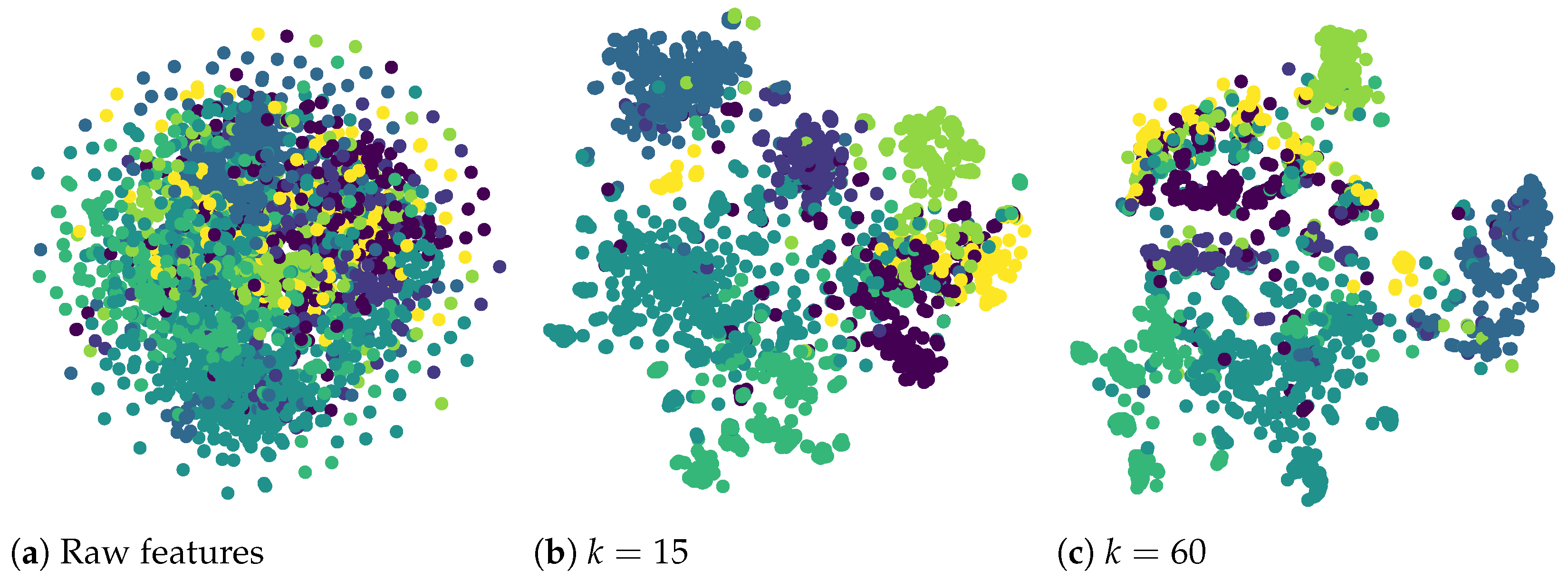
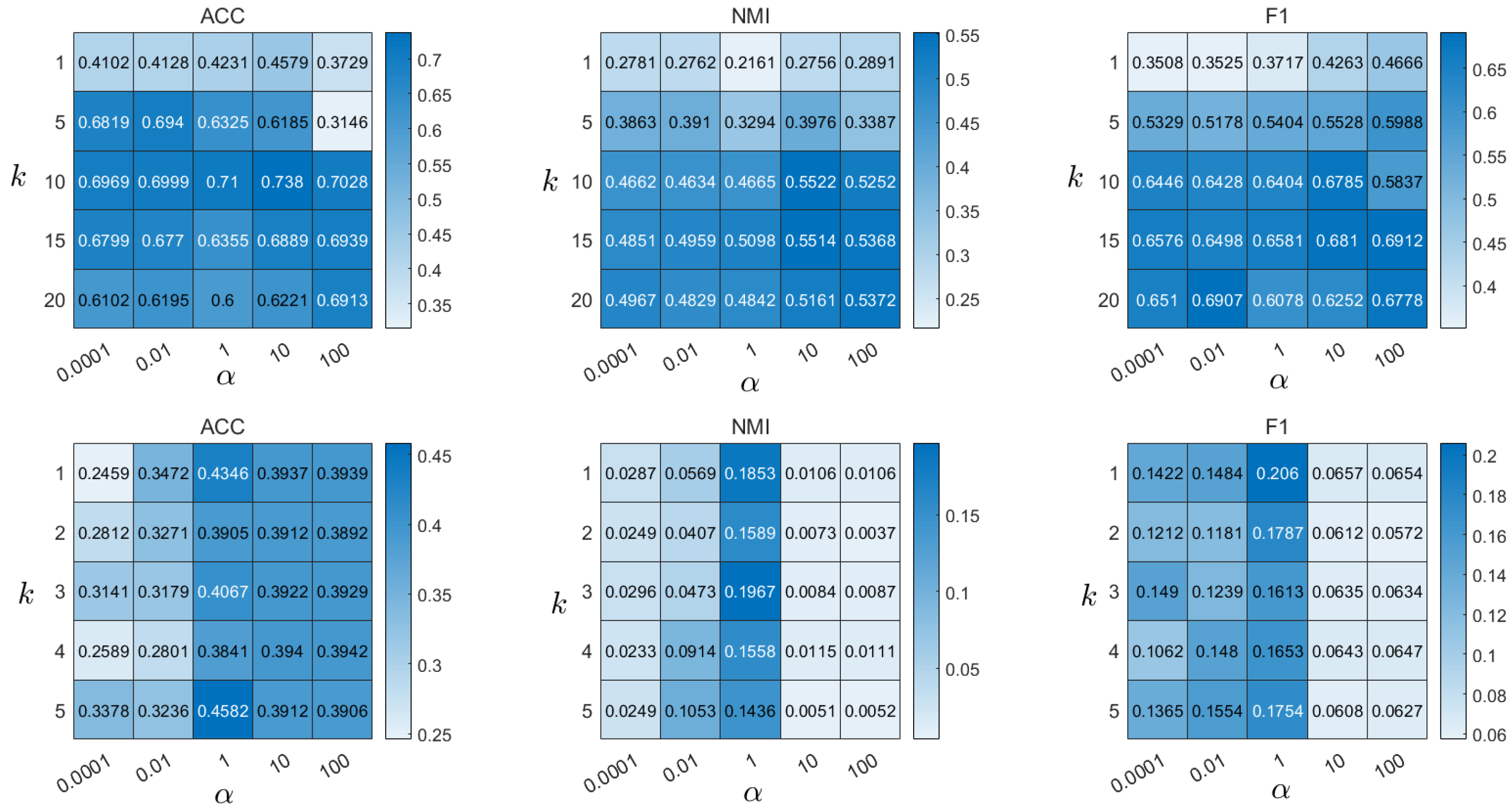
We analyze the sensitivity of parameters in our model. The unsampled model (5) involves the filter order k and the balance parameter $\alpha$. When k increases, nearby node features become similar. However, too large k will lead to over-smoothing, where the features of nodes in different clusters are mixed and become indistinguishable, harming the performance. In fact, over-smoothing is commonly seen in GCN and is intensively studied recently. To visualize it, we use t-SNE on Cora’s raw and filtered node features in Figure 1. We can see clear cluster patterns at $k=15$, but the cluster structures vanish when the features are oversmoothed at $k=60$. The impacts of k and $\alpha$ on clustering performance are shown in Figure 2. A small k range and a wide $\alpha$ range can produce a rational outcome.

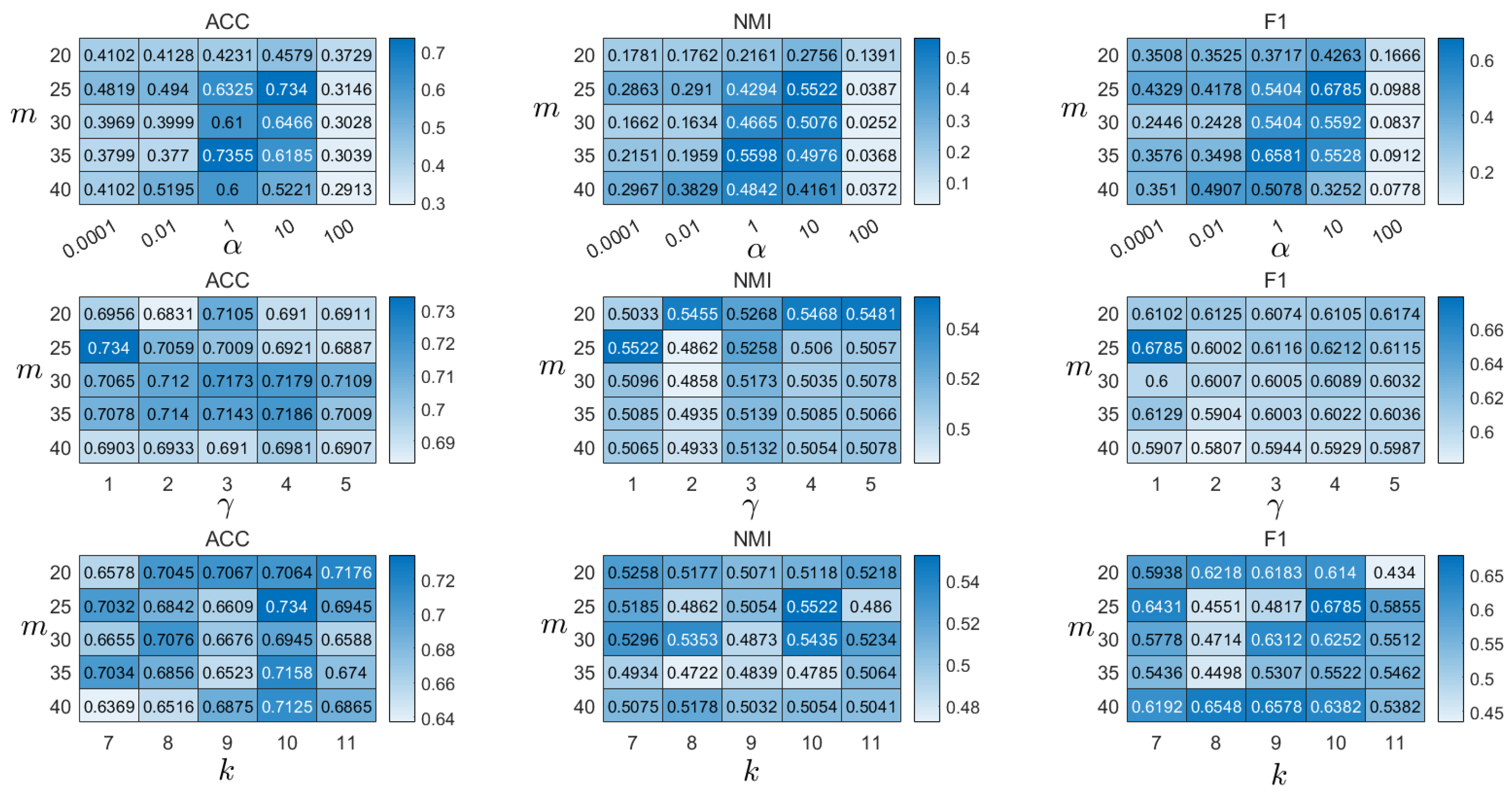
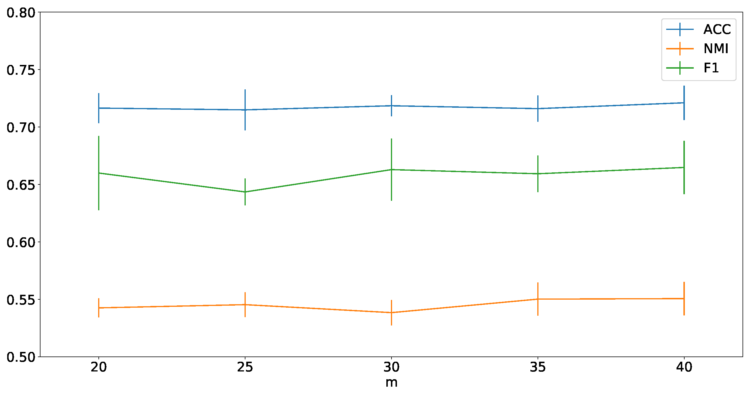
The sampling-based model (7) has several parameters to tune, including the balance parameter $\alpha$, the filter order k, the sampling parameter $\gamma$, and the number of anchors m. We show the clustering results under various parameter values in Figure 3. To obtain each value, we fix two parameters and tune the other two. We can see that our method works well for a wide range of parameter values. Specifically, it can be seen that the results are sensitive to $\alpha$, which indicates that it is important to find a good balance between attribute and structure information and that exploiting only one type of information could not achieve the best performance. Besides, k is less sensitive compared to the unsampled approach, which is a reasonable result because only a small part of the nodes are chosen. $\gamma$ does not have too much impact on the results, which makes parameter tuning easy. To better visualize the influence of the anchor number, we all fix m and tune other parameters. From Figure 4, we can find that m has a small influence. In principle, m could not be less than the number of clusters. By contrast, too large m will make the anchors less representative.

5. Conclusions

In this work, we propose a graph learning-based attributed graph clustering method. It has several distinct properties. First, it follows a graph learning approach, which makes it be flexible enough to suit different datasets. Second, it learns a smaller graph and performs SVD on a smaller matrix, so that it enjoys the advantage of linear complexity with respect to the number of nodes. Third, a novel anchor selecting method is developed to incorporate the different roles of nodes. Fourth, it is capable of exploiting different orders of complex relationships, which is important for different datasets. Extensive experiments verify the superiority of our proposed method, in terms of effectiveness and efficiency. In particular, the proposed method generally performs better than deep learning based methods and consumes much less time. Therefore, our method is a promising attributed graph clustering technique.

References

- Fang, R.; Wen, L.; Kang, Z.; Liu, J. Structure-Preserving Graph Representation Learning. In Proceedings of the IEEE International Conference on Data Mining (ICDM), Orlando, FL, USA, 28 November–1 December 2022. [Google Scholar]
- Cao, S.; Lu, W.; Xu, Q. Deep neural networks for learning graph representations. In Proceedings of the Thirtieth AAAI Conference on Artificial Intelligence, Phoenix, AZ, USA, 12–17 February 2016. [Google Scholar]
- Wang, C.; Pan, S.; Long, G.; Zhu, X.; Jiang, J. Mgae: Marginalized graph autoencoder for graph clustering. In Proceedings of the 2017 ACM on Conference on Information and Knowledge Management, Singapore, 6–10 November 2017; pp. 889–898. [Google Scholar]
- Kang, Z.; Lin, Z.; Zhu, X.; Xu, W. Structured graph learning for scalable subspace clustering: From single view to multiview. IEEE Trans. Cybern. 2022, 52, 8976–8986. [Google Scholar] [CrossRef] [PubMed]
- Liu, L.; Kang, Z.; Ruan, J.; He, X. Multilayer graph contrastive clustering network. Inf. Sci. 2022, 613, 256–267. [Google Scholar] [CrossRef]
- Xu, Z.; Ke, Y.; Wang, Y.; Cheng, H.; Cheng, J. A model-based approach to attributed graph clustering. In Proceedings of the 2012 ACM SIGMOD International Conference on Management of Data, San Diego, CA, USA, 20 May 2012; pp. 505–516. [Google Scholar]
- Huang, S.; Kang, Z.; Xu, Z.; Liu, Q. Robust deep k-means: An effective and simple method for data clustering. Pattern Recognit. 2021, 117, 107996. [Google Scholar] [CrossRef]
- Murtagh, F.; Contreras, P. Algorithms for hierarchical clustering: An overview. Wiley Interdiscip. Rev. Data Min. Knowl. Discov. 2012, 2, 86–97. [Google Scholar] [CrossRef]
- Guo, T.; Pan, S.; Zhu, X.; Zhang, C. CFOND: Consensus factorization for co-clustering networked data. IEEE Trans. Knowl. Data Eng. 2018, 31, 706–719. [Google Scholar] [CrossRef]
- Liu, L.; Xu, L.; Wangy, Z.; Chen, E. Community detection based on structure and content: A content propagation perspective. In Proceedings of the 2015 IEEE International Conference on Data Mining, Atlantic City, NJ, USA, 14 November 2015; pp. 271–280. [Google Scholar]
- Chang, J.; Blei, D. Relational topic models for document networks. In Artificial Intelligence and Statistics; Addison-Wesley: Boston, MA, USA, 2009; pp. 81–88. [Google Scholar]
- Liu, C.; Wen, L.; Kang, Z.; Luo, G.; Tian, L. Self-supervised consensus representation learning for attributed graph. In Proceedings of the 29th ACM International Conference on Multimedia, Chengdu, China, 20 October 2021; pp. 2654–2662. [Google Scholar]
- Kipf, T.N.; Welling, M. Variational graph auto-encoders. arXiv 2016, arXiv:1611.07308. [Google Scholar]
- Pan, S.; Hu, R.; Fung, S.f.; Long, G.; Jiang, J.; Zhang, C. Learning graph embedding with adversarial training methods. IEEE Trans. Cybern. 2019, 50, 2475–2487. [Google Scholar] [CrossRef] [PubMed] [Green Version]
- Tian, F.; Gao, B.; Cui, Q.; Chen, E.; Liu, T.Y. Learning deep representations for graph clustering. In Proceedings of the AAAI Conference on Artificial Intelligence, Quebec City, QC, Canada, 27–30 July 2014; Volume 28. [Google Scholar]
- Hui, B.; Zhu, P.; Hu, Q. Collaborative Graph Convolutional Networks: Unsupervised Learning Meets Semi-Supervised Learning. AAAI Tech. Track Mach. Learn. 2020, 34, 4215–4222. [Google Scholar] [CrossRef]
- Wang, C.; Pan, S.; Hu, R.; Long, G.; Jiang, J.; Zhang, C. Attributed Graph Clustering: A Deep Attentional Embedding Approach. arXiv 2019, arXiv:1906.06532. [Google Scholar]
- Henaff, M.; Bruna, J.; LeCun, Y. Deep convolutional networks on graph-structured data. arXiv 2015, arXiv:1506.05163. [Google Scholar]
- Pan, E.; Kang, Z. Multi-view Contrastive Graph Clustering. Adv. Neural Inf. Process. Syst. 2021, 34, 2148–2159. [Google Scholar]
- Liu, Y.; Gao, Q.; Yang, Z.; Wang, S. Learning with Adaptive Neighbors for Image Clustering. In Proceedings of the Twenty-Seventh International Joint Conference on Artificial Intelligence, Stockholm, Sweden, 13–19 July 2018; pp. 2483–2489. [Google Scholar]
- Mathisen, B.M.; Aamodt, A.; Bach, K.; Langseth, H. Learning similarity measures from data. Prog. Artif. Intell. 2020, 9, 129–143. [Google Scholar] [CrossRef] [Green Version]
- Kang, Z.; Liu, Z.; Pan, S.; Tian, L. Fine-grained Attributed Graph Clustering. In Proceedings of the 2022 SIAM International Conference on Data Mining (SDM), Minneapolis, MN, USA, 27–29 April 2022; pp. 370–378. [Google Scholar]
- Bianchi, F.M.; Grattarola, D.; Alippi, C. Spectral clustering with graph neural networks for graph pooling. In Proceedings of the International Conference on Machine Learning, Seoul, Republic of Korea, 25–28 October 2020; pp. 874–883. [Google Scholar]
- He, D.; Feng, Z.; Jin, D.; Wang, X.; Zhang, W. Joint identification of network communities and semantics via integrative modeling of network topologies and node contents. In Proceedings of the Thirty-First AAAI Conference on Artificial Intelligence, San Francisco, CA, USA, 4–9 February 2017. [Google Scholar]
- Chunaev, P. Community detection in node-attributed social networks: A survey. Comput. Sci. Rev. 2020, 37, 100286. [Google Scholar] [CrossRef]
- Wang, C.; Pan, S.; Celina, P.Y.; Hu, R.; Long, G.; Zhang, C. Deep neighbor-aware embedding for node clustering in attributed graphs. Pattern Recognit. 2022, 122, 108230. [Google Scholar] [CrossRef]
- Zhang, X.; Liu, H.; Li, Q.; Wu, X.M. Attributed Graph Clustering via Adaptive Graph Convolution. In Proceedings of the Twenty-Eighth International Joint Conference on Artificial Intelligence, Macao, China, 10–16 August 2019. [Google Scholar]
- Ma, Z.; Kang, Z.; Luo, G.; Tian, L.; Chen, W. Towards Clustering-friendly Representations: Subspace Clustering via Graph Filtering. In Proceedings of the 28th ACM International Conference on Multimedia, Athlone, Ireland, 26–28 May 2020; pp. 3081–3089. [Google Scholar]
- Chung, F.R.; Graham, F.C. Spectral Graph Theory; Number 92; American Mathematical Soc.: Providence, RI, USA, 1997. [Google Scholar]
- Dong, X.; Thanou, D.; Rabbat, M.; Frossard, P. Learning graphs from data: A signal representation perspective. IEEE Signal Process. Mag. 2019, 36, 44–63. [Google Scholar] [CrossRef] [Green Version]
- Ortega, A.; Frossard, P.; Kovačević, J.; Moura, J.M.; Vandergheynst, P. Graph signal processing: Overview, challenges, and applications. Proc. IEEE 2018, 106, 808–828. [Google Scholar] [CrossRef] [Green Version]
- Kang, Z.; Lu, X.; Liang, J.; Bai, K.; Xu, Z. Relation-Guided Representation Learning. Neural Netw. 2020, 131, 93–102. [Google Scholar] [CrossRef] [PubMed]
- Lin, Z.; Kang, Z.; Zhang, L.; Tian, L. Multi-view Attributed Graph Clustering. IEEE Trans. Knowl. Data Eng. 2021; early access. [Google Scholar] [CrossRef]
- Bo, D.; Wang, X.; Shi, C.; Zhu, M.; Lu, E.; Cui, P. Structural deep clustering network. In Proceedings of the Web Conference 2020, Taipei, Taiwan, 20–24 April 2020; pp. 1400–1410. [Google Scholar]
- Cao, S.; Lu, W.; Xu, Q. Grarep: Learning graph representations with global structural information. In Proceedings of the 24th ACM International on Conference on Information and Knowledge Management, Melbourne, Australia, 19–23 October 2015; pp. 891–900. [Google Scholar]
- Kang, Z.; Zhou, W.; Zhao, Z.; Shao, J.; Han, M.; Xu, Z. Large-Scale Multi-View Subspace Clustering in Linear Time. In Proceedings of the AAAI Conference on Artificial Intelligence, New York, NY, USA, 7–12 February 2020; pp. 4412–4419. [Google Scholar]
- Chen, X.; Cai, D. Large scale spectral clustering with landmark-based representation. In Proceedings of the Twenty-Fifth AAAI Conference on Artificial Intelligence, San Francisco, CA, USA, 7–11 August 2011. [Google Scholar]
- Mikolov, T.; Sutskever, I.; Chen, K.; Corrado, G.S.; Dean, J. Distributed representations of words and phrases and their compositionality. In Advances in Neural Information Processing Systems; Mit Pr: Cambridge, MA, USA, 2013; pp. 3111–3119. [Google Scholar]
- Malliaros, F.D.; Giatsidis, C.; Papadopoulos, A.N.; Vazirgiannis, M. The core decomposition of networks: Theory, algorithms and applications. VLDB J. 2020, 29, 61–92. [Google Scholar] [CrossRef]
- Yang, C.; Liu, Z.; Zhao, D.; Sun, M.; Chang, E. Network representation learning with rich text information. In Proceedings of the Twenty-Fourth International Joint Conference on Artificial Intelligence, Buenos Aires, Argentina, 25–31 July 2015. [Google Scholar]
- Li, Q.; Wu, X.M.; Liu, H.; Zhang, X.; Guan, Z. Label Efficient Semi-Supervised Learning via Graph Filtering. In Proceedings of the Conference on Computer Vision and Pattern Recognition, Long Beach, CA, USA, 15–20 June 2019. [Google Scholar]
- Wang, X.; Cui, P.; Wang, J.; Pei, J.; Zhu, W.; Yang, S. Community preserving network embedding. In Proceedings of the Thirty-First AAAI Conference on Artificial Intelligence, San Francisco, CA, USA, 4–9 February 2017. [Google Scholar]
- Perozzi, B.; Al-Rfou, R.; Skiena, S. Deepwalk: Online learning of social representations. In Proceedings of the 20th ACM SIGKDD International Conference on Knowledge Discovery and Data Mining, New York, NY, USA, 24–27 August 2014; pp. 701–710. [Google Scholar]
- Pan, S.; Hu, R.; Long, G.; Jiang, J.; Yao, L.; Zhang, C. Adversarially regularized graph autoencoder for graph embedding. In Proceedings of the Twenty-Seventh International Joint Conference on Artificial Intelligence, Stockholm, Sweden, 13–19 July 2018. [Google Scholar]
- Zhu, Q.; Du, B.; Yan, P. Multi-hop Convolutions on Weighted Graphs. arXiv 2019, arXiv:1911.04978. [Google Scholar]
Figure 1.
t-SNE demonstration of the raw and filtered node features of Cora dataset.
Figure 2.
The influence of parameters k and on results of Cora (first row) and Large Cora (second row) datasets in FGC.
Figure 3.
The influence of parameters on the results of the Cora dataset in GLGC.
Figure 4.
The influence of m on the results of the Cora dataset in GLGC. The error bar denotes the standard deviation of 10 tests.