On New Generalized Viscosity Implicit Double Midpoint Rule for Hierarchical Problem

Abstract

The implicit midpoint rules are employed as a powerful numerical technique, and in this article we attend a class of viscosity iteration approximations on hierarchical problems for the implicit double midpoint rules. We prove the strong convergence theorem to the unique solution on hierarchical problem of this technique is established under some favorable conditions imposed on the control parameters in Hilbert spaces. Furthermore, we propose some applications to the constrained convex minimization problem, nonlinear Fredholm integral equation and variational inequality on fixed point problem. Moreover, some numerical examples are also presented to illustrate the different proposed methods and convergence results. Our results modified the implicit double midpoint rules with the hierarchical problem.

1. Introduction

To begin with, we first give some necessary notations that we use throughout our paper. In the framework of a real Hilbert space H with inner product $\langle ·,·\rangle$ and its induced norm $\parallel ·\parallel$, let C be a subset of H with its properties which are closed and convex. The notations ⇀ and → refer to weak convergence and strong convergence, respectively.

Next, we recall some definitions which will be considered in the next part of our paper. We shall start with the well-known problem referred to as The variational inequality [1] which is to find the solution $x^{*}\in C$ that satisfies the following inequality

$$\begin{array}{c}\hfill \langle A{x}^{*},x-x^{*}\rangle \ge 0,\forall x\in C,\end{array}$$

where C is nonempty. The set of its solution is denoted by $VI(C,A)$, that is,

$$\begin{array}{c}\hfill VI(C,A)=\left\{x^{*}\in C:\langle A{x}^{*},x-x^{*}\rangle \ge 0,\forall x\in C\right\}.\end{array}$$

The contraction mapping $f:C\to C$ with a constant $\rho \in [0,1)$ is defined as follows: for all $x,y\in C$

$$\begin{array}{c}\hfill \parallel f\left(x\right)-f\left(y\right)\parallel \le \rho \parallel x-y\parallel .\end{array}$$

A self-mapping on H, A, is said to be $\alpha$-strongly monotone if there exists a positive real number $\alpha$ satisfying

$$\begin{array}{c}\hfill \langle Ax-Ay,x-y\rangle \ge {\alpha \parallel x-y\parallel }^2,\forall x,y\in H.\end{array}$$

A self-mapping on H is called L-Lipschitz continuous if there exists a real number $L>0$ such that for all $x,y$ in H which satisfies the following:

$$\begin{array}{c}\hfill \parallel Ax-Ay\parallel \le L\parallel x-y\parallel .\end{array}$$

An operator A which is linear and bounded is titled as a strongly positive on H if there exists a positive constant $\overline{\gamma }$ that meets the following inequality:

$$\begin{array}{c}\hfill \langle Ax,x\rangle \ge \overline{\gamma }{\parallel x\parallel }^2,\forall x\in H.\end{array}$$

A well-known nonexpansive mapping, T, is defined by

$$\begin{array}{c}\hfill \parallel Tx-Ty\parallel \le \parallel x-y\parallel \end{array}$$

for all elements $x,y$ in C.

We shall say that a point x in C is a fixed point of a mapping T when that x satisfies the equality $Tx=x$. Undoubtedly, for any mapping T, there may be one or various or no fixed point. However, where it is present we will denote the set of its fixed point as $Fix\left(T\right)$, i.e., $Fix\left(T\right)=\{x\in C:$$Tx=x\}$.

For a nonexpansive mapping $T:C\to C$ where C is bounded, closed and convex, $Fix\left(T\right)$ is exactly nonempty [2].

Recently, since the variational inequality problem has attracted many mathematicians to find the best way to solve it, there arose a new interesting problem, known as the hierarchical problem, that was improved from the classical variational inequality. Instead of considering the variational inequality over a closed convex set C, we mention that problem over the fixed point set of a nonexpansive mapping $T:C\to C$. This problem can be stated as follows:

Let $A:C\to H$ and $T:C\to C$ be a monotone continuous mapping and a nonexpansive mapping, respectively. This hierarchical problem is to find $x^{*}\in Fix\left(T\right)$ which satisfies

$$\begin{array}{c}\hfill \langle A{x}^{*},x-x^{*}\rangle \ge 0,\forall x\in Fix\left(T\right),\end{array}$$

where $Fix\left(T\right)$ is nonempty and we aim to denote its solution set as $VI\left(Fix\right(T),A)$. There are many researches involving this problem in the literature [3,4,5,6,7,8,9,10,11,12,13,14,15,16,17].

In 2011, Yao et.al [18] proposed an iterative algorithm that provides a strong convergence to a unique solution of variational in equality in case of hierarchical problem. Their iterative algorithm for generating the sequence $\left\{x_n\right\}$ is designed by

$$\begin{array}{c}\hfill x_{n+1}={\beta }_n{x}_n+(1-{\beta }_n)T{P}_C[I-{\alpha }_n(A-\gamma f)]x_n,\forall n\ge 0,\end{array}$$

where $x_0\in C$ is chosen arbitrarily and both sequence $\left\{{\alpha }_n\right\}$ and $\left\{{\beta }_n\right\}$ are in $[0,1]$. Under some appropriate assumptions, they can gaurantee that the generated sequence converges to a unique solution $x^{*}\in Fix\left(T\right)$ of the following variational inequality:

$$\begin{array}{c}\hfill \langle (A-\gamma f)x^{*},x-x^{*}\rangle \ge 0,\forall x\in Fix\left(T\right)\end{array}$$

(1)

where $A:C\to H$ which is a strongly positive linear bounded operator, $f:C\to H$ is a $\rho$-contraction and $T:C\to C$ which is a nonexpansive mapping where $Fix\left(T\right)$ is nonempty. They identified the solution set of (1) by ${\Omega }_1:=VI(Fix\left(T\right),A-\gamma f)$.

Later, in 2011, Ceng et.al [19] studied a strong convergence to a unique solution of the variational inequality on the modified hierarchical problem. For $x_0\in C$ which is chosen arbitrarily, define a sequence $\left\{x_n\right\}$ followed by

$$\begin{array}{c}\hfill x_{n+1}=P_C[{\lambda }_n\gamma ({\alpha }_{n}f\left(x_n\right)+(1-{\alpha }_n)S{x}_n)+(I-{\lambda }_n\mu F)T{x}_n],\forall n\ge 0,\end{array}$$

(2)

where the sequences $\left\{{\alpha }_n\right\}$ and $\left\{{\lambda }_n\right\}$ in $[0,1].$ Then, $\left\{x_n\right\}$ converges strongly to $x^{*}\in Fix\left(T\right)$ which is the unique solution of the variational inequality which is to find $x^{*}\in Fix\left(T\right)$ satisfying

$$\begin{array}{c}\hfill \langle (\mu F-\gamma )x^{*},x-x^{*}\rangle \ge 0,\forall x\in Fix\left(T\right).\end{array}$$

(3)

By algorithm (2), the assumption of an $F:C\to H$ is a Lipschitzian and strongly monotone operator, $f:C\to H$ is a contraction mapping, $S,T$ are both nonexpansive mappings with $Fix\left(T\right)$ being nonempty and others satisfying certain conditions. They give a notation of the solution set of (3) as ${\Omega }_2:=VI(Fix\left(T\right),\mu F-\gamma )$.

Next, in 2014, Kumam and Jitpeera [20] consider a strong convergence to a unique solution of the hybrid hierarchical problem. They generated the sequence $\left\{x_n\right\}$ iteratively as follows:

$$\begin{array}{c}\hfill x_{n+1}=\gamma {\lambda }_n\varphi \left(x_n\right)+(I-{\lambda }_n\mu F)T{P}_C[{\beta }_{n}S{x}_n+(1-{\beta }_n)x_n],\forall n\ge 0,\end{array}$$

(4)

where $x_0\in C$ can be chosen arbitrarily and both sequences $\left\{{\beta }_n\right\}$ and $\left\{{\lambda }_n\right\}$ in $[0,1].$ They found that the generated sequence $\left\{x_n\right\}$ converges strongly to a unique solution $x^{*}\in Fix\left(T\right)$ of the following vriational inequality:

$$\begin{array}{c}\hfill \mathrm{Find}{x}^{*}\in Fix\left(T\right)\mathrm{such}\mathrm{that}\langle (\mu F-\gamma \varphi )x^{*},x-x^{*}\rangle \ge 0,\forall x\in Fix\left(T\right),\end{array}$$

(5)

where $F:C\to H$ is a Lipschitzian and strongly monotone operator, $\varphi :C\to C$ is a contraction mapping and $S,T$ are nonexpansive mappings with $Fix\left(T\right)$ is nonempty. The solution set of (5) is denoted by ${\Omega }_3:=VI(Fix\left(T\right),\mu F-\gamma \varphi )$.

In recent years, the implicit midpoint rule has been proved in many papers [21,22]. The implicit midpoint rule is one of the powerful methods for finding ordinary differential equations. In 2019, Dhakal and Sintunavarat [23] studied the viscosity method to the implicit double midpoint rule for nonexpansive mapping. For $x_0\in C$ is chosen arbitrarily, the sequences $\left\{x_n\right\}$ be generated by the following algorithm,

$$\begin{array}{c}\hfill x_{n+1}={\alpha }_{n}f\left(\frac{x_n+x_{n+1}}{2}\right)-(1-{\alpha }_n)T\left(\frac{x_n+x_{n+1}}{2}\right),\forall n\ge 0,\end{array}$$

where the sequences ${\alpha }_n\in (0,1).$ Under some mild conditions, they can show that the generated sequence $\left\{x_n\right\}$ converges strongly to a unique solution $x^{*}\in Fix\left(T\right)$ of the following variational inequality.

$$\begin{array}{c}\hfill \mathrm{Find}{x}^{*}\in Fix\left(T\right)\mathrm{such}\mathrm{that}\langle (I-f)x^{*},x-x^{*}\rangle \ge 0,\forall x\in Fix\left(T\right),\end{array}$$

(6)

where $f:C\to C$ is a contraction mapping and T is nonexpansive mapping with $Fix\left(T\right)$ is a nonempty set. They denoted ${\Omega }_4:=VI(Fix\left(T\right),I-f)$ as the solution set of (6).

By considering the previous mentioned research, we aim to consider a hybrid viscosity method using implicit double midpoint rule to solve a hybrid hierarchical problems, stated as follows:

$$\begin{array}{c}\hfill \left\{\begin{array}{c}{y}_n=P_C[{\beta }_{n}S{x}_n+(1-{\beta }_n)x_{n+1}],\hfill \\ x_{n+1}=\gamma {\lambda }_n\varphi (w_n{x}_n+(1-w_n)x_{n+1})+(I-{\lambda }_n\mu F)T{y}_n,\forall n\ge 0,\hfill \end{array}\right.\end{array}$$

(7)

where $S,T$ are nonexpansive mappings with $F\left(T\right)$ is nonempty, $F:C\to H$ is a Lipschitzian and strongly monotone operator, $\varphi :H\to H$ is a contraction mapping and other control sequences satisfy some mild conditions. Our mentioned problem is stated as follows:

$$\begin{array}{c}\hfill \mathrm{Find}{x}^{*}\in Fix\left(T\right)\mathrm{such}\mathrm{that}\langle (\mu F-\gamma \varphi )x^{*},x-x^{*}\rangle \ge 0,\forall x\in Fix\left(T\right).\end{array}$$

We also give the notation of its solutions set by $\Omega :=VI\left(Fix\right(T),\mu F-\gamma \varphi )$, that is

$$VI(Fix\left(T\right),\mu F-\gamma \varphi )=\left\{x^{*}\in Fix\left(T\right):\langle (\mu F-\gamma \varphi )x^{*},x-x^{*}\rangle \ge 0,\forall x\in Fix\left(T\right)\right\}.$$

Under some appropriate assumptions, we exactly claim the strong convergence of our sequence $\left\{x_n\right\}$ generated by our proposed algorithm. The results improve the main theorem of Dhakal and Sintunavarat [23], Kumam and Jitpeera [20]. Thus, our solution is $VI\left(Fix\right(T),\mu F-\gamma \varphi )$, which is more general than $VI\left(Fix\right(T),I-f)$. Furthermore, our new algorithm (7) is more general than (4) that uses the double midpoint rule.

The remainder of this paper is divided into six sections. In Section 1, we recall some definitions and properties to be used in the sequel. In Section 2, lemmas are provided for using in proof. In Section 3, we prove the strong convergence theorem of the hybrid hierarchical problem with double midpoint rules in the Hilbert spaces. Some deduced results are provided in Section 4. In Section 5, we present some applications and numerical examples. The conclusion is given in the final section.

2. Preliminaries

In this section, we collect some definitions, properties and lemmas that are necessary for use in this paper. We start with the following inequality: ${\parallel x+y\parallel }^2\le {\parallel x\parallel }^2+2\langle y,x+y\rangle ,$$\forall x,y\in H.$

An operator $P_C:H\to C$, that project every point $x\in H$ to a unique nearest point in C is called the metric projection of H onto C, that is, $P_{C}x=min\{\left.∥x-y\parallel ,y\in C\right\}.$ From it definitions, it is trivial that the following properties hold.

$$\langle x-y,P_{C}x-P_{C}y\rangle \ge {\parallel P_{C}x-P_{C}y\parallel }^2,\forall x,y\in H.$$

$$\langle x-P_{C}x,y-P_{C}x\rangle \le 0,\forall x,y\in H.$$

(8)

$${\parallel x-y\parallel }^2\ge \parallel x-P_C{x\parallel }^2+{\parallel y-P_{C}x\parallel }^2,\forall x,y\in H.$$

Furthermore, for a monotone mapping $A:C\to H$, the properties (8) implies that

$$x^{*}\in VI(C,A)\iff x^{*}=P_C(x^{*}-\lambda A{x}^{*}),\lambda >0.$$

Next, we recall some lemmas that will be used in the proof.

Lemma 1

([24]). Let $\left\{a_n\right\}$ be a sequence of nonnegative real numbers such that

$$a_{n+1}\le (1-{\gamma }_n)a_n+{\delta }_n,\forall n\ge 0,$$

where $\left\{{\gamma }_n\right\}\subset (0,1)$ and $\left\{{\delta }_n\right\}$ is a sequence in $\mathbb{R}$ such that

(i) ${\sum }_{n=1}^{\infty }{\gamma }_n=\infty$,

(ii) ${lim\; sup}_{n\to \infty }\frac{{\delta }_n}{{\gamma }_n}\le 0$ or ${\sum }_{n=1}^{\infty }\left|{\delta }_n\right|<\infty .$

Then ${lim}_{n\to \infty }{a}_n=0$.

Lemma 2

([25]). Let C be a nonempty closed and convex subset of a real Hilbert space H, and $T:C\to C$ be a nonexpansive mapping with $Fix\left(T\right)\ne \varnothing .$ If $\left\{x_n\right\}$ is a sequence in C such that $\{x-n\}\}$ converges weakly to x and $\left\{(I-T)x_n\right\}$ converges strongly to 0, where I is the identity mapping, then $Tx=x.$

3. Main Results

In this section, we propose our algorithm for solving hierarchical problem by using technique of the viscosity method together with a generalized implicit double midpoint rule. We also verify the strong convergence of our generated sequence to a fixed point of nonexpansive mapping which is also a unique solution of a mentioned variational inequality.

Theorem 1.

Let C be a nonempty closed and convex subset of a real Hilbert space H. $F:C\to C$ be κ-Lipschitzian and η-strongly monotone operators with constant κ and $\eta >0$. $\varphi :C\to C$ be a ρ-contraction with coefficient $\rho \in [0,1)$. $T:C\to C$ be a nonexpansive mapping with $Fix\left(T\right)\ne \varnothing$, $S:H\to H$ be a nonexpansive mapping. Let $0<\mu <2\eta /{\kappa }^2$ and $0<\gamma <\tau$, where $\tau =1-\sqrt{1-\mu (2\eta -\mu {\kappa }^2)}$. Suppose $\left\{x_n\right\}$ is a sequence generated by the following algorithm which $x_0\in C$ is chosen arbitrarily,

$$\begin{array}{c}\hfill \left\{\begin{array}{c}{y}_n=P_C[{\beta }_{n}S{x}_n+(1-{\beta }_n)x_{n+1}],\hfill \\ x_{n+1}=\gamma {\lambda }_n\varphi (w_n{x}_n+(1-w_n)x_{n+1})+(I-{\lambda }_n\mu F)T{y}_n,\forall n\ge 0,\hfill \end{array}\right.\end{array}$$

(9)

where $\left\{{\lambda }_n\right\}\subset (0,1)$, $\left\{{\beta }_n\right\},\left\{w_n\right\}\subset (0.5,1)$ satisfy the following conditions:

(C1): ${\beta }_n\le k{\lambda }_n$;

(C2): ${lim}_{n\to \infty }{\lambda }_n=0$, ${lim}_{n\to \infty }\frac{{\lambda }_n-{\lambda }_{n-1}}{{\lambda }_n}=0$, ${\sum }_{n=0}^{\infty }{\lambda }_n=\infty$;

(C3): ${lim}_{n\to \infty }\frac{{\beta }_n-{\beta }_{n-1}}{{\beta }_n}=0$.

Then, $\left\{x_n\right\}$ converges strongly to $x^{*}\in Fix\left(T\right)$, which is the unique solution of another variational inequality:

$$\langle (\mu F-\gamma \varphi )x^{*},x-x^{*}\rangle \ge 0,\forall x\in Fix\left(T\right),$$

where $\Omega =VI\left(Fix\right(T),\mu F-\gamma \varphi )\ne \varnothing$. On the other hand, $x^{*}$ is a unique fixed point $P_{Fix\left(T\right)}(\gamma \varphi -\mu F),$ that is, $P_{Fix\left(T\right)}(\gamma \varphi -\mu F)\left(x^{*}\right)=x^{*}$

Proof. 

First, we want to show the existence of a sequence $\left\{x_n\right\}$ defined by (9). Consider the mapping $S_n:C\to C$ by $S_{n}x=\gamma {\lambda }_n\varphi (w_{n}w+(1-w_n)x)+(I-{\lambda }_n\mu F)T{P}_C[{\beta }_{n}Sw+(1-{\beta }_n)x]$ for all $x\in C.$ We will show the mapping $S_n$ is a contraction mapping for all $n\in \mathrm{N}.$ For each $n\in \mathrm{N}$ and $x,y\in C,$ we have

$$\begin{array}{ccc}\hfill \parallel S_{n}x-S_{n}y\parallel & =& \parallel \gamma {\lambda }_n\varphi (w_{n}w+(1-w_n)x)+(I-{\lambda }_n\mu F)T{P}_C[{\beta }_{n}Sw+(1-{\beta }_n)x]\hfill \\ & & -\gamma {\lambda }_n\varphi (w_{n}w+(1-w_n)y)-(I-{\lambda }_n\mu F)T{P}_C[{\beta }_{n}Sw+(1-{\beta }_n)y]\parallel \hfill \\ & \le & \gamma {\lambda }_n\parallel \varphi (w_{n}w+(1-w_n)x)-\varphi (w_{n}w+(1-w_n)y)\parallel \hfill \\ & & +(I-{\lambda }_n\mu F)\parallel T{P}_C[{\beta }_{n}Sw+(1-{\beta }_n)x]-T{P}_C[{\beta }_{n}Sw+(1-{\beta }_n)y]\parallel \hfill \\ & \le & \rho \gamma {\lambda }_n\parallel (w_{n}w+(1-w_n)x)-(w_{n}w+(1-w_n)y)\parallel \hfill \\ & & +(1-{\lambda }_n\tau )\parallel [{\beta }_{n}Sw+(1-{\beta }_n)x]-[{\beta }_{n}Sw+(1-{\beta }_n)y]\parallel \hfill \\ & \le & \rho \gamma {\lambda }_n\parallel (1-w_n)x-(1-w_n)y\parallel +(1-{\lambda }_n\tau )\parallel (1-{\beta }_n)x-(1-{\beta }_n)y\parallel \hfill \\ & \le & \rho \gamma {\lambda }_n(1-w_n)\parallel x-y\parallel +(1-{\lambda }_n\tau )(1-{\beta }_n)\parallel x-y\parallel \hfill \\ & =& [\rho \gamma {\lambda }_n(1-w_n)+(1-{\lambda }_n\tau )(1-{\beta }_n)]\parallel x-y\parallel \hfill \\ & =& \acute{\rho }\parallel x-y\parallel ,\hfill \end{array}$$

where $\acute{\rho }=\rho \gamma {\lambda }_n(1-w_n)+(1-{\lambda }_n\tau )(1-{\beta }_n)\in [0,1)$ for all $n\in \mathrm{N}.$ This shows that the mapping $S_n$ is a contraction mapping for all $n\in \mathrm{N}.$ From the Banach contraction principle, $S_n$ has a unique fixed point for all $n\in \mathrm{N}.$ Thus, we conclude the existence of a sequence $\left\{x_n\right\}$ defined by (9). We will divide the proof into six steps.

Step 1. First, we claim that $\left\{x_n\right\}$ is bounded. Indeed, for any $x^{*}\in Fix\left(T\right)$, we can see that

$$\begin{array}{ccc}\hfill \parallel x_{n+1}-x^{*}\parallel & =& \parallel \gamma {\lambda }_n\varphi (w_n{x}_n+(1-w_n)x_{n+1})\hfill \\ & & +(I-{\lambda }_n\mu F)T{P}_C[{\beta }_{n}S{x}_n+(1-{\beta }_n)x_{n+1}]-x^{*}\parallel \hfill \\ & \le & \gamma {\lambda }_n\parallel \varphi (w_n{x}_n+(1-w_n)x_{n+1})-\varphi x^{*}\parallel \hfill \\ & & +(I-{\lambda }_n\mu F)\parallel T{P}_C[{\beta }_{n}S{x}_n+(1-{\beta }_n)x_{n+1}]-T{P}_C{x}^{*}\parallel \hfill \\ & \le & \gamma \rho {\lambda }_n\{w_n\parallel x_n-x^{*}\parallel +(1-w_n)\parallel x_{n+1}-x^{*}\parallel \}+{\lambda }_n\parallel \gamma \varphi x^{*}-\mu F{x}^{*}\parallel \hfill \\ & & +(1-{\lambda }_n\tau )·\hfill \\ & & \{{\beta }_n\parallel x_n-x^{*}\parallel +(1-{\beta }_n)\parallel x_{n+1}-x^{*}\parallel +{\beta }_n\parallel S{x}^{*}-x^{*}\parallel \}\hfill \\ & =& (\gamma \rho {\lambda }_n{w}_n+(1-{\lambda }_n\tau ){\beta }_n)\parallel x_n-x^{*}\parallel \hfill \\ & & +(\gamma \rho {\lambda }_n(1-w_n)+(1-{\lambda }_n\tau )(1-{\beta }_n))\parallel x_{n+1}-x^{*}\parallel \hfill \\ & & +(1-{\lambda }_n\tau ){\beta }_n\parallel S{x}^{*}-x^{*}\parallel +{\lambda }_n\parallel \gamma \varphi x^{*}-\mu F{x}^{*}\parallel \hfill \\ & \le & \frac{\gamma \rho {\lambda }_n{w}_n+(1-{\lambda }_n\tau ){\beta }_n}{\gamma \rho {\lambda }_n{w}_n+(1-{\lambda }_n\tau ){\beta }_n+{\lambda }_n(\tau -\gamma \rho )}\parallel x_n-x^{*}\parallel \hfill \\ & & +\frac{(1-{\lambda }_n\tau ){\beta }_n}{\gamma \rho {\lambda }_n{w}_n+(1-{\lambda }_n\tau ){\beta }_n+{\lambda }_n(\tau -\gamma \rho )}\parallel S{x}^{*}-x^{*}\parallel \hfill \\ & & +\frac{{\lambda }_n}{\gamma \rho {\lambda }_n{w}_n+(1-{\lambda }_n\tau ){\beta }_n+{\lambda }_n(\tau -\gamma \rho )}\parallel \gamma \varphi x^{*}-\mu F{x}^{*}\parallel \hfill \\ & \le & \left(1-\frac{{\lambda }_n(\tau -\gamma \rho )}{\gamma \rho {\lambda }_n{w}_n+(1-{\lambda }_n\tau ){\beta }_n+{\lambda }_n(\tau -\gamma \rho )}\right)\parallel x_n-x^{*}\parallel \hfill \\ & & +\frac{k{\lambda }_n(\tau -\gamma \rho )}{\gamma \rho {\lambda }_n{w}_n+(1-{\lambda }_n\tau ){\beta }_n+{\lambda }_n(\tau -\gamma \rho )}·\frac{1}{\tau -\gamma \rho }\parallel S{x}^{*}-x^{*}\parallel \hfill \\ & & +\frac{{\lambda }_n(\tau -\gamma \rho )}{\gamma \rho {\lambda }_n{w}_n+(1-{\lambda }_n\tau ){\beta }_n+{\lambda }_n(\tau -\gamma \rho )}·\frac{1}{\tau -\gamma \rho }\parallel \gamma \varphi x^{*}-\mu F{x}^{*}\parallel \hfill \\ & \le & \left(1-\frac{{\lambda }_n(\tau -\gamma \rho )}{\gamma \rho {\lambda }_n{w}_n+(1-{\lambda }_n\tau ){\beta }_n+{\lambda }_n(\tau -\gamma \rho )}\right)\parallel x_n-x^{*}\parallel \hfill \\ & & +\frac{{\lambda }_n(\tau -\gamma \rho )}{\gamma \rho {\lambda }_n{w}_n+(1-{\lambda }_n\tau ){\beta }_n+{\lambda }_n(\tau -\gamma \rho )}·\hfill \\ & & \left(\frac{k}{\tau -\gamma \rho }\parallel S{x}^{*}-x^{*}\parallel +\frac{1}{\tau -\gamma \rho }\parallel \gamma \varphi x^{*}-\mu F{x}^{*}\parallel \right)\hfill \\ & \le & max\left\{\parallel x_n-x^{*}\parallel ,\frac{1}{\tau -\gamma \rho }(k\parallel S{x}^{*}-x^{*}\parallel +\parallel \gamma \varphi x^{*}-\mu F{x}^{*}\parallel )\right\}.\hfill \end{array}$$

By induction, it follows that

$$\begin{array}{ccc}\hfill \parallel x_n-x^{*}\parallel & \le & max\left\{\parallel x_0-x^{*}\parallel ,\frac{1}{\tau -\gamma \rho }(k\parallel S{x}^{*}-x^{*}\parallel +\parallel \gamma \varphi x^{*}-\mu F{x}^{*}\parallel )\right\},n\ge 0.\hfill \end{array}$$

Therefore, $\left\{x_n\right\}$ is bounded.

Step 2. We verify that ${lim}_{n\to \infty }\parallel x_{n+1}-x_n\parallel =0$. For each $n\in \mathrm{N}$ with $n>1$, we obtain

$$\begin{array}{ccc}\hfill \parallel x_{n+1}-x_n\parallel & =& \parallel \gamma {\lambda }_n\varphi (w_n{x}_n+(1-w_n)x_{n+1})+(I-{\lambda }_n\mu F)T{P}_C[{\beta }_{n}S{x}_n+(1-{\beta }_n)x_{n+1}]\hfill \\ & & -\gamma {\lambda }_{n-1}\varphi (w_{n-1}{x}_{n-1}+(1-w_{n-1})x_n)\hfill \\ & & -(I-{\lambda }_{n-1}\mu F)T{P}_C[{\beta }_{n-1}S{x}_{n-1}+(1-{\beta }_{n-1})x_n]\parallel .\hfill \end{array}$$

So that

$$\begin{array}{ccc}\hfill \parallel x_{n+1}-x_n\parallel & =& \parallel \gamma {\lambda }_n\left(\varphi (w_n{x}_n+(1-w_n)x_{n+1})-\varphi (w_{n-1}{x}_{n-1}+(1-w_{n-1})x_n)\right)\hfill \\ & & +\gamma ({\lambda }_n-{\lambda }_{n-1})\varphi (w_{n-1}{x}_{n-1}+(1-w_{n-1})x_n)\hfill \\ & & +(I-{\lambda }_n\mu F)·\hfill \\ & & \left(T{P}_C[{\beta }_{n}S{x}_n+(1-{\beta }_n)x_{n+1}]-T{P}_C[{\beta }_{n-1}S{x}_{n-1}+(1-{\beta }_{n-1})x_n]\right)\hfill \\ & & +\mu ({\lambda }_{n-1}-{\lambda }_n)FT{P}_C[{\beta }_{n-1}S{x}_{n-1}+(1-{\beta }_{n-1})x_n]\parallel \hfill \\ & \le & \gamma \rho {\lambda }_n\parallel (1-w_n)(x_{n+1}-x_n)+w_{n-1}(x_n-x_{n-1})\parallel \hfill \\ & & +\gamma |{\lambda }_n-{\lambda }_{n-1}|\parallel \varphi (w_{n-1}{x}_{n-1}+(1-w_{n-1})x_n)\parallel \hfill \\ & & +(1-{\lambda }_n\tau )·\hfill \\ & & \parallel (1-{\beta }_n)(x_{n+1}-x_n)+{\beta }_n(S{x}_n-S{x}_{n-1})+({\beta }_n-{\beta }_{n-1})(S{x}_{n-1}-x_n)\parallel \hfill \\ & & +\mu |{\lambda }_n-{\lambda }_{n-1}|\parallel FT{P}_C[{\beta }_{n-1}S{x}_{n-1}+(1-{\beta }_{n-1})x_n]\parallel \hfill \\ & \le & \left(\gamma \rho {\lambda }_n(1-w_n)+(1-{\lambda }_n\tau )(1-{\beta }_n)\right)\parallel x_{n+1}-x_n\parallel \hfill \\ & & +\left(\gamma \rho {\lambda }_n{w}_{n-1}+(1-{\lambda }_n\tau ){\beta }_n\right)\parallel x_n-x_{n-1}\parallel \hfill \\ & & +|{\lambda }_n-{\lambda }_{n-1}\{\gamma \parallel \varphi (w_{n-1}{x}_{n-1}+(1-w_{n-1})x_n)\parallel \hfill \\ & & +\mu \parallel FT{P}_C[{\beta }_{n-1}S{x}_{n-1}+(1-{\beta }_{n-1})x_n]\parallel \}\hfill \\ & & +(1-{\lambda }_n\tau )|{\beta }_n-{\beta }_{n-1}|\parallel S{x}_{n-1}-x_n\parallel \hfill \\ & =& \left(\gamma \rho {\lambda }_n(1-w_n)+(1-{\lambda }_n\tau )(1-{\beta }_n)\right)\parallel x_{n+1}-x_n\parallel \hfill \\ & & +\left(\gamma \rho {\lambda }_n{w}_{n-1}+(1-{\lambda }_n\tau ){\beta }_n\right)\parallel x_n-x_{n-1}\parallel \hfill \\ & & +|{\lambda }_n-{\lambda }_{n-1}|M_1+(1-{\lambda }_n\tau )|{\beta }_n-{\beta }_{n-1}|M_2,\hfill \\ & \le & \frac{\gamma \rho {\lambda }_n{w}_{n-1}+(1-{\lambda }_n\tau ){\beta }_n}{\gamma \rho {\lambda }_n{w}_n+(1-{\lambda }_n\tau ){\beta }_n+{\lambda }_n(\tau -\gamma \rho )}\parallel x_n-x_{n-1}\parallel \hfill \\ & & +\frac{|{\lambda }_n-{\lambda }_{n-1}|}{\gamma \rho {\lambda }_n{w}_n+(1-{\lambda }_n\tau ){\beta }_n+{\lambda }_n(\tau -\gamma \rho )}{M}_1\hfill \\ & & +\frac{(1-{\lambda }_n\tau )|{\beta }_n-{\beta }_{n-1}|}{\gamma \rho {\lambda }_n{w}_n+(1-{\lambda }_n\tau ){\beta }_n+{\lambda }_n(\tau -\gamma \rho )}{M}_2\hfill \\ & =& \left(1-\frac{{\lambda }_n(\tau -\gamma \rho )}{\gamma \rho {\lambda }_n{w}_n+(1-{\lambda }_n\tau ){\beta }_n+{\lambda }_n(\tau -\gamma \rho )}\right)\parallel x_n-x_{n-1}\parallel \hfill \\ & & +\frac{|{\lambda }_n-{\lambda }_{n-1}|}{\gamma \rho {\lambda }_n{w}_n+(1-{\lambda }_n\tau ){\beta }_n+{\lambda }_n(\tau -\gamma \rho )}{M}_1\hfill \\ & & +\frac{(1-{\lambda }_n\tau )|{\beta }_n-{\beta }_{n-1}|}{\gamma \rho {\lambda }_n{w}_n+(1-{\lambda }_n\tau ){\beta }_n+{\lambda }_n(\tau -\gamma \rho )}{M}_2,\hfill \end{array}$$

which $M_1:={sup}_{n\in \mathrm{N}}\left\{\gamma \parallel \varphi (w_{n-1}{x}_{n-1}+(1-w_{n-1})x_n)\parallel +\mu \parallel FT{P}_C[{\beta }_{n-1}S{x}_{n-1}+(1-{\beta }_{n-1})x_n]\parallel \right\}$ and $M_2:=\parallel S{x}_{n-1}-x_n\parallel .$ This yields that for all $n\in \mathrm{N}$ with $n>1$. We can also write

$$\begin{array}{ccc}\hfill \parallel x_{n+1}-x_n\parallel & \le & (1-{\alpha }_n)\parallel x_n-x_{n-1}\parallel +{\delta }_n\hfill \end{array}$$

(10)

for all $n\in \mathrm{N}$ with $n>1$, where

$${\alpha }_n:=\frac{{\lambda }_n(\tau -\gamma \rho )}{\gamma \rho {\lambda }_n{w}_n+(1-{\lambda }_n\tau ){\beta }_n+{\lambda }_n(\tau -\gamma \rho )}$$

and

$${\delta }_n:=\frac{|{\lambda }_n-{\lambda }_{n-1}|}{\gamma \rho {\lambda }_n{w}_n+(1-{\lambda }_n\tau ){\beta }_n+{\lambda }_n(\tau -\gamma \rho )}{M}_1+\frac{(1-{\lambda }_n\tau )|{\beta }_n-{\beta }_{n-1}|}{\gamma \rho {\lambda }_n{w}_n+(1-{\lambda }_n\tau ){\beta }_n+{\lambda }_n(\tau -\gamma \rho )}{M}_2.$$

Using the conditions (C1), (C2) and comparing (10) with Lemma 1, we obtain

$$\begin{array}{c}\hfill \underset{n\to \infty }{lim}\parallel x_{n+1}-x_n\parallel =0.\end{array}$$

(11)

Step 3. We want to show that ${lim}_{n\to \infty }\parallel x_n-T{x}_n\parallel =0$. For each $n\in \mathrm{N}$, we have

$$\begin{array}{ccc}\hfill \parallel x_n-T{x}_n\parallel & \le & \parallel x_n-x_{n+1}\parallel +\parallel x_{n+1}-T{P}_C[{\beta }_{n}S{x}_n+(1-{\beta }_n)x_{n+1}]\parallel \hfill \\ & & +\parallel T{P}_C[{\beta }_{n}S{x}_n+(1-{\beta }_n)x_{n+1}]-T{x}_n\parallel \hfill \\ & \le & \parallel x_n-x_{n+1}\parallel \hfill \\ & & +{\lambda }_n\parallel \gamma \varphi (w_n{x}_n+(1-w_n)x_{n+1})-\mu FT{P}_C[{\beta }_{n}S{x}_n+(1-{\beta }_n)x_{n+1}]\parallel \hfill \\ & & +\parallel {\beta }_{n}S{x}_n+(1-{\beta }_n)x_{n+1}-x_n\parallel \hfill \\ & \le & \parallel x_n-x_{n+1}\parallel \hfill \\ & & +{\lambda }_n\left\{\gamma \parallel \varphi (w_n{x}_n+(1-w_n)x_{n+1})\parallel +\mu \parallel FT{P}_C[{\beta }_{n}S{x}_n+(1-{\beta }_n)x_{n+1}]\parallel \right\}\hfill \\ & & +(1-{\beta }_n)\parallel x_n-x_{n+1}\parallel +{\beta }_n\parallel x_n-S{x}_n\parallel \hfill \\ & \le & \parallel x_n-x_{n+1}\parallel +{\lambda }_n{M}_1\hfill \\ & & +(1-{\beta }_n)\parallel x_n-x_{n+1}\parallel +{\beta }_n\parallel x_n-x_{n+1}\parallel +{\beta }_n\parallel x_{n+1}-S{x}_n\parallel \hfill \\ & \le & 2\parallel x_n-x_{n+1}\parallel +{\lambda }_n{M}_1+{\beta }_n{M}_2.\hfill \end{array}$$

From the conditions (C1), (C2) and using (11), we obtain

$$\begin{array}{c}\hfill \underset{n\to \infty }{lim}\parallel x_n-T{x}_n\parallel =0.\end{array}$$

(12)

Step 4. We need to claim that ${\omega }_w\left(x_n\right)\subseteq Fix\left(T\right)$, where

$$\begin{array}{c}\hfill {\omega }_w\left(x_n\right):=\{x\in H:\exists \left\{x_{n_i}\right\}\rightharpoonup x\}.\end{array}$$

Let us consider $x\in {\omega }_w\left(x_n\right).$ Then there exists a subsequence $\left\{x_{n_i}\right\}$ of $\left\{x_n\right\}$ such that $x_{n_i}\rightharpoonup x$. From (12), we obtain

$$\begin{array}{c}\hfill \underset{i\to \infty }{lim}\parallel (I-T)x_{n_i}\parallel =\underset{n\to \infty }{lim}\parallel x_{n_i}-T{x}_{n_i}\parallel =0.\end{array}$$

It implies that $\left\{(I-T)x_{n_i}\right\}$ strong convergence to 0. Using Lemma 2, we obtain $Tx=x$ and $x\in Fix\left(T\right)$. Thus, we can conclude that ${\omega }_w\left(x_n\right)\subseteq Fix\left(T\right).$

Step 5. We want to show that

$$\begin{array}{c}\hfill \underset{n\to \infty }{lim\; sup}\langle x^{*}-\varphi \left(x^{*}\right),x^{*}-x_n\rangle \le 0,\end{array}$$

where $x^{*}\in Fix\left(T\right)$ is a unique fixed point of $P_{Fix\left(T\right)}\circ \varphi ,$ that is $x^{*}=P_{Fix\left(T\right)}\varphi \left(x^{*}\right).$ Since $\left\{x_n\right\}$ is bounded, there exists a subsequence $\left\{x_{n_i}\right\}$ of $\left\{x_n\right\}$ such that it has weak convergence to $p.$ Without loss of generality, we may assume that $x_{n_i}\rightharpoonup p$ as $i\to \infty$ for some $p\in H$ and

$$\begin{array}{c}\hfill \underset{n\to \infty }{lim\; sup}\langle x^{*}-\varphi \left(x^{*}\right),x^{*}-x_n\rangle =\underset{i\to \infty }{lim}\langle x^{*}-\varphi \left(x^{*}\right),x^{*}-x_{n_i}\rangle .\end{array}$$

From the Step 4, we obtain $p\in Fix\left(T\right)$. Using (8), we obtain

$$\begin{array}{c}\hfill \underset{n\to \infty }{lim\; sup}\langle x^{*}-\varphi \left(x^{*}\right),x^{*}-x_n\rangle =\underset{i\to \infty }{lim}\langle x^{*}-\varphi \left(x^{*}\right),x^{*}-x_{n_i}\rangle =\langle x^{*}-\varphi \left(x^{*}\right),x^{*}-p\rangle \le 0.\end{array}$$

Step 6. Finally, we will prove $x_{n+1}\to x^{*}$. From (9), we note that

$$\begin{array}{ccc}\hfill \parallel x_{n+1}-x^{*}{\parallel }^2& =& \parallel \gamma {\lambda }_n\varphi (w_n{x}_n+(1-w_n)x_{n+1})\hfill \\ & & +(I-{\lambda }_n\mu F)T{P}_C[{\beta }_{n}S{x}_n+(1-{\beta }_n)x_{n+1}]-x^{*}{\parallel }^2\hfill \\ & =& \parallel \gamma {\lambda }_n\left(\varphi (w_n{x}_n+(1-w_n)x_{n+1})-\varphi x^{*}\right)\hfill \\ & & +(I-{\lambda }_n\mu F)\left(T{P}_C[{\beta }_{n}S{x}_n+(1-{\beta }_n)x_{n+1}]-x^{*}\right)+{\lambda }_n(\gamma \varphi x^{*}-\mu F{x}^{*}){\parallel }^2\hfill \\ & \le & \parallel \gamma {\lambda }_n\left(\varphi (w_n{x}_n+(1-w_n)x_{n+1})-\varphi x^{*}\right)\hfill \\ & & +(I-{\lambda }_n\mu F)\left(T{P}_C[{\beta }_{n}S{x}_n+(1-{\beta }_n)x_{n+1}]-x^{*}\right){\parallel }^2\hfill \\ & & +2{\lambda }_n\langle \gamma \varphi x^{*}-\mu F{x}^{*},x_{n+1}-x^{*}\rangle \hfill \\ & \le & {\gamma }^2{\lambda }_n^2{\parallel \varphi (w_n{x}_n+(1-w_n)x_{n+1})-\varphi x^{*}\parallel }^2\hfill \\ & & +{(1-{\lambda }_n\tau )}^2{\parallel T{P}_C[{\beta }_{n}S{x}_n+(1-{\beta }_n)x_{n+1}]-x^{*}\parallel }^2\hfill \\ & & +2\gamma {\lambda }_n(1-{\lambda }_n\tau )·\hfill \\ & & \langle \varphi (w_n{x}_n+(1-w_n)x_{n+1})-\varphi x^{*},T{P}_C[{\beta }_{n}S{x}_n+(1-{\beta }_n)x_{n+1}]-x^{*}\rangle \hfill \\ & & +2{\lambda }_n\langle \gamma \varphi x^{*}-\mu F{x}^{*},x_{n+1}-x^{*}\rangle \hfill \\ & \le & {\gamma }^2{\rho }^2{\lambda }_n^2{\parallel w_n(x_n-x^{*})+(1-w_n)(x_{n+1}-x^{*})\parallel }^2+{\eta }_n\hfill \\ & & +2\gamma \rho {\lambda }_n(1-{\lambda }_n\tau )\parallel w_n(x_n-x^{*})+(1-w_n)(x_{n+1}-x^{*})\parallel ·\hfill \\ & & \parallel {\beta }_n(x_n-x^{*})+(1-{\beta }_n)(x_{n+1}-x^{*})+{\beta }_n(S{x}^{*}-x^{*})\parallel \hfill \\ & \le & {\gamma }^2{\rho }^2{\lambda }_n^2(w_n^2\parallel x_n-x^{*}{\parallel }^2+w_n(1-w_n)(\parallel x_n-x^{*}{\parallel }^2+\parallel x_{n+1}-x^{*}{\parallel }^2)\hfill \\ & & +{(1-w_n)}^2{\parallel x_{n+1}-x^{*}\parallel }^2)\hfill \\ & & +2\gamma \rho {\lambda }_n(1-{\lambda }_n\tau )(w_n{\beta }_n\parallel x_n-x^{*}{\parallel }^2+(w_n(1-{\beta }_n)+(1-w_n){\beta }_n)\hfill \\ & & \parallel x_n-x^{*}\parallel \parallel x_{n+1}-x^{*}\parallel +(1-w_n)(1-{\beta }_n){\parallel x_{n+1}-x^{*}\parallel }^2)\hfill \\ & & +2\gamma \rho {\lambda }_n{\beta }_n(1-{\lambda }_n\tau )\parallel S{x}^{*}-x^{*}\parallel \left(w_n\parallel x_n-x^{*}\parallel +(1-w_n)\parallel x_{n+1}-x^{*}\parallel \right)\hfill \\ & & +{\eta }_n\hfill \\ & \le & {\gamma }^2{\rho }^2{\lambda }_n^2{w}_n\parallel x_n-x^{*}{\parallel }^2+{\gamma }^2{\rho }^2{\lambda }_n^2(1-w_n){\parallel x_{n+1}-x^{*}\parallel }^2\hfill \\ & & +2\gamma \rho {\lambda }_n(1-{\lambda }_n\tau )w_n{\beta }_n{\parallel x_n-x^{*}\parallel }^2\hfill \\ & & +2\gamma \rho {\lambda }_n(1-{\lambda }_n\tau )(1-w_n)(1-{\beta }_n){\parallel x_{n+1}-x^{*}\parallel }^2\hfill \\ & & +\gamma \rho {\lambda }_n(1-{\lambda }_n\tau )(w_n(1-{\beta }_n)+(1-w_n){\beta }_n)·\hfill \\ & & \left(\parallel x_n-x^{*}{\parallel }^2+{\parallel x_{n+1}-x^{*}\parallel }^2\right)\hfill \\ & & +2\gamma \rho {\lambda }_n{\beta }_n(1-{\lambda }_n\tau )\parallel S{x}^{*}-x^{*}\parallel \left(w_n\parallel x_n-x^{*}\parallel +(1-w_n)\parallel x_{n+1}-x^{*}\parallel \right)\hfill \\ & & +{\eta }_n\hfill \\ & \le & \left({\gamma }^2{\rho }^2{\lambda }_n^2{w}_n+2\gamma \rho {\lambda }_n(1-{\lambda }_n\tau )w_n{\beta }_n\right){\parallel x_n-x^{*}\parallel }^2\hfill \\ & & +\left({\gamma }^2{\rho }^2{\lambda }_n^2(1-w_n)+2\gamma \rho {\lambda }_n(1-{\lambda }_n\tau )(1-w_n)(1-{\beta }_n)\right){\parallel x_{n+1}-x^{*}\parallel }^2\hfill \\ & & +\gamma \rho {\lambda }_n(1-{\lambda }_n\tau )(w_n(1-{\beta }_n)+(1-w_n){\beta }_n)\parallel x_n-x^{*}{\parallel }^2\hfill \\ & & +\gamma \rho {\lambda }_n(1-{\lambda }_n\tau )(w_n(1-{\beta }_n)+(1-w_n){\beta }_n)\parallel x_{n+1}-x^{*}{\parallel }^2\hfill \\ & & +2\gamma \rho {\lambda }_n{\beta }_n(1-{\lambda }_n\tau )\parallel S{x}^{*}-x^{*}\parallel \left(w_n\parallel x_n-x^{*}\parallel +(1-w_n)\parallel x_{n+1}-x^{*}\parallel \right)\hfill \\ & & +{\eta }_n.\hfill \end{array}$$

Hence

$$\begin{array}{ccc}\hfill \parallel x_{n+1}-x^{*}{\parallel }^2& =& \left({\gamma }^2{\rho }^2{\lambda }_n^2{w}_n+\gamma \rho {\lambda }_n(1-{\lambda }_n\tau )(w_n+{\beta }_n)\right){\parallel x_n-x^{*}\parallel }^2\hfill \\ & & +\left({\gamma }^2{\rho }^2{\lambda }_n^2(1-w_n)+\gamma \rho {\lambda }_n(1-{\lambda }_n\tau )(2-w_n-{\beta }_n)\right){\parallel x_{n+1}-x^{*}\parallel }^2\hfill \\ & & +2\gamma \rho {\lambda }_n{\beta }_n(1-{\lambda }_n\tau )\parallel S{x}^{*}-x^{*}\parallel \left(w_n\parallel x_n-x^{*}\parallel +(1-w_n)\parallel x_{n+1}-x^{*}\parallel \right)\hfill \\ & & +{\eta }_n,\hfill \end{array}$$

where

$${\eta }_n:={(1-{\lambda }_n\tau )}^2{\parallel T{P}_C[{\beta }_{n}S{x}_n+(1-{\beta }_n)x_{n+1}]-x^{*}\parallel }^2+2{\lambda }_n\langle \gamma \varphi x^{*}-\mu F{x}^{*},x_{n+1}-x^{*}\rangle .$$

This implies that

$$\begin{array}{ccc}\hfill \parallel x_{n+1}-x^{*}{\parallel }^2& \le & \frac{{\gamma }^2{\rho }^2{\lambda }_n^2{w}_n+\gamma \rho {\lambda }_n(1-{\lambda }_n\tau )(w_n+{\beta }_n)}{1-\left({\gamma }^2{\rho }^2{\lambda }_n^2(1-w_n)+\gamma \rho {\lambda }_n(1-{\lambda }_n\tau )(2-w_n-{\beta }_n)\right)}{\parallel x_n-x^{*}\parallel }^2\hfill \\ & & +\frac{2\gamma \rho {\lambda }_n{\beta }_n(1-{\lambda }_n\tau )\parallel S{x}^{*}-x^{*}\parallel \left(w_n\parallel x_n-x^{*}\parallel +(1-w_n)\parallel x_{n+1}-x^{*}\parallel \right)}{1-\left({\gamma }^2{\rho }^2{\lambda }_n^2(1-w_n)+\gamma \rho {\lambda }_n(1-{\lambda }_n\tau )(2-w_n-{\beta }_n)\right)}\hfill \\ & & +\frac{{(1-{\lambda }_n\tau )}^2{\parallel T{P}_C[{\beta }_{n}S{x}_n+(1-{\beta }_n)x_{n+1}]-x^{*}\parallel }^2}{1-\left({\gamma }^2{\rho }^2{\lambda }_n^2(1-w_n)+\gamma \rho {\lambda }_n(1-{\lambda }_n\tau )(2-w_n-{\beta }_n)\right)}\hfill \\ & & +\frac{(2{\lambda }_n\langle \gamma \varphi x^{*}-\mu F{x}^{*},x_{n+1}-x^{*}\rangle }{1-\left({\gamma }^2{\rho }^2{\lambda }_n^2(1-w_n)+\gamma \rho {\lambda }_n(1-{\lambda }_n\tau )(2-w_n-{\beta }_n)\right)}\hfill \end{array}$$

This completes the proof. □

4. Some Deduced Results

Corollary 1.

Let C be a nonempty closed and convex subset of a real Hilbert space H. $F:C\to C$ be κ-Lipschitzian and η-strongly monotone operators with constant κ and $\eta >0$. Let $T:C\to C$ be a nonexpansive mapping with $Fix\left(T\right)\ne \varnothing$, $S:H\to H$ be a nonexpansive mapping. Let the control conditions be $0<\mu <2\eta /{\kappa }^2$ and $0<\gamma <\tau$, where $\tau =1-\sqrt{1-\mu (2\eta -\mu {\kappa }^2)}$. Suppose the generated sequence $\left\{x_n\right\}$ is designed by the following algorithm where $x_0\in C$ can be chosen arbitrarily:

$$\begin{array}{c}\hfill x_{n+1}=(I-{\lambda }_n\mu F)T{P}_C[{\beta }_{n}S{x}_n+(1-{\beta }_n)x_{n+1}],\forall n\ge 0,\end{array}$$

where $\left\{{\lambda }_n\right\}\subset (0,1)$, $\left\{{\beta }_n\right\},\subset (0.5,1)$ satisfy conditions (C1)–(C3). Then, $\left\{x_n\right\}$ converges strongly to $x^{*}\in Fix\left(T\right)$, which is the unique solution of variational inequality:

$$\langle (\mu F-I)x^{*},x-x^{*}\rangle \ge 0,\forall x\in Fix\left(T\right),$$

where ${\Omega }_a=VI(Fix\left(T\right),\mu F-I)\ne \varnothing$. On the other hand, $x^{*}$ is a unique fixed point $P_{Fix\left(T\right)}$$(I-\mu F),$ that is, $P_{Fix\left(T\right)}(I-\mu F)\left(x^{*}\right)=x^{*}$.

Proof. 

Putting $\varphi \equiv 0$ into Theorem 1, we can immediately obtain the desired result. □

Corollary 2.

Let C be a nonempty closed and convex subset of a real Hilbert space H. $\varphi :H\to H$ be a ρ-contraction with coefficient $\rho \in [0,1)$, $T:C\to C$ be a nonexpansive mapping with $Fix\left(T\right)\ne \varnothing$ and $S:H\to H$ be a nonexpansive mapping. Suppose $\left\{x_n\right\}$ is a sequence generated by the following algorithm $x_0\in C$ arbitrarily:

$$\left\{\begin{array}{c}{y}_n=P_C[{\beta }_{n}S{x}_n+(1-{\beta }_n)x_{n+1}],\hfill \\ x_{n+1}={\lambda }_n\varphi (w_n{x}_n+(1-w_n)x_{n+1})+(1-{\lambda }_n)T{y}_n,\forall n\ge 0,\hfill \end{array}\right.$$

where $\left\{{\lambda }_n\right\}\subset (0,1)$, $\left\{{\beta }_n\right\},\left\{w_n\right\}\subset (0.5,1)$ satisfy the following conditions (C1)–(C3). Then, $\left\{x_n\right\}$ converges strongly to $x^{*}\in Fix\left(T\right)$, which is the unique solution of variational inequality:

$$\langle (I-\varphi )x^{*},x-x^{*}\rangle \ge 0,\forall x\in Fix\left(T\right),$$

where ${\Omega }_b=VI(Fix\left(T\right),I-\varphi )\ne \varnothing$. On the other hand, $x^{*}$ is a unique fixed point $P_{Fix\left(T\right)}(\varphi -I),$ that is, $P_{Fix\left(T\right)}(\varphi -I)\left(x^{*}\right)=x^{*}$.

Proof. 

Putting $\gamma =1,\mu =2$ and $F\equiv \frac{I}{2}$ in Theorem 1, we can immediately obtain the desired result. □

Corollary 3.

Let C be a nonempty closed and convex subset of a real Hilbert space H. $T:C\to C$ be a nonexpansive mapping with $Fix\left(T\right)\ne \varnothing$ and $S:H\to H$ be a nonexpansive mapping. Suppose $\left\{x_n\right\}$ is a sequence generated by the following algorithm $x_0\in C$ arbitrarily:

$$x_{n+1}=(1-{\lambda }_n)T{P}_C[{\beta }_{n}S{x}_n+(1-{\beta }_n)x_{n+1}],\forall n\ge 0,$$

where $\left\{{\beta }_n\right\}\subset (0.5,1)$ satisfy the following condition (C1)-(C3). Then $\left\{x_n\right\}$ converges strongly to $x^{*}\in Fix\left(T\right)$, which is the unique solution of variational inequality:

$$\langle (I-S)x^{*},x-x^{*}\rangle \ge 0,\forall x\in Fix\left(T\right).$$

where ${\Omega }_c=VI(Fix\left(T\right),I-S)\ne \varnothing$. On the other hand, $x^{*}$ is a unique fixed point $P_{Fix\left(T\right)}(S-I),$ that is, $P_{Fix\left(T\right)}(S-I)\left(x^{*}\right)=x^{*}$.

Proof. 

Putting $\varphi \equiv 0$ and in Corollary 2, we can immediately obtain the desired result. □

Corollary 4.

Let C be a nonempty closed and convex subset of a real Hilbert space H. $T:C\to C$ be a nonexpansive mapping with $Fix\left(T\right)\ne \varnothing$ and $S:C\to C$ be a nonexpansive mapping. Suppose $\left\{x_n\right\}$ is a sequence generated by the following algorithm $x_0\in C$ arbitrarily:

$$x_{n+1}={\lambda }_n{x}_n+(1-{\lambda }_n)T[{\beta }_{n}S{x}_n+(1-{\beta }_n)x_n],\forall n\ge 0,$$

where $\left\{{\lambda }_n\right\}\subset (0,1)$, $\left\{{\beta }_n\right\}\subset (0.5,1)$ satisfy the following conditions (C1)-(C3). Then $\left\{x_n\right\}$ converges strongly to $x^{*}\in Fix\left(T\right)$, which is the unique solution of variational inequality:

$$\langle (I-S)x^{*},x-x^{*}\rangle \ge 0,\forall x\in Fix\left(T\right).$$

where ${\Omega }_d=VI(Fix\left(T\right),I-S)\ne \varnothing$. On the other hand, $x^{*}$ is a unique fixed point $P_{Fix\left(T\right)}(S-I),$ that is, $P_{Fix\left(T\right)}(S-I)\left(x^{*}\right)=x^{*}$.

Proof. 

Putting $\varphi \equiv I,$$\left\{w_n\right\}=1,$$P_C\equiv I$ in Corollary 2, we can immediately obtain the desired result. □

5. Applications and Numerical

5.1. Nonlinear Fredholm Integral Equation

In this part, we consider the following nonlinear Fredholm integral equation:

$$x\left(r\right)=h\left(r\right)+{\int }_0^{1}Q(r,t,x\left(t\right))dt,\forall r\in [0,1],$$

(13)

where h is a continuous function on the interval $[0,1].$

$Q:[0,1]\times [0,1]\times \mathbb{R}\to \mathbb{R}$ is a continuous function. In this case, if we assume that Q satisfies the Lipschitz continuity condition, i.e.,

$$\left|Q\right(r,t,x)-Q(r,t,y\left)\right|\le |x-y|,\forall r,t\in [0,1],x,y\in \mathbb{R},$$

then we can verify that Equation (13) has at least one solution in $L_2[0,1]$ (see [26], Theorem 3.3). Define the mappings $S,T:L_2[0,1]\to L_2[0,1]$ by:

$$\left(Sx\right)\left(r\right)=h\left(r\right)+{\int }_0^{1}Q(r,t,x\left(t\right))dt,\forall r\in [0,1],$$

(14)

and

$$\left(Tx\right)\left(r\right)=h\left(r\right)+{\int }_0^{1}Q(r,t,x\left(t\right))dt,\forall r\in [0,1].$$

(15)

Then, for any $x,y\in L_2[0,1],$ we have:

$$\begin{array}{ll}{\parallel Sx-Ty\parallel }^2& ={\int }_0^1{|\left(Sx\right)\left(r\right)-\left(Ty\right)\left(r\right)|}^{2}dr\\ & ={\int }_0^1{\left|{\int }_0^{1}Q(r,t,x\left(t\right))-Q(r,t,y\left(t\right))dt\right|}^{2}dr\\ & \le {\int }_0^1{\left|{\int }_0^1\left|x\left(t\right)-y\left(t\right)\right|dt\right|}^{2}dr\\ & \le {\int }_0^1{\left|x\left(t\right)-y\left(t\right)\right|}^{2}dt\\ & \le {\parallel x-y\parallel }^2,\end{array}$$

which implies that S and T are nonexpansive mapping on $L_2[0,1].$ We can definitely say that the solution finding of Equation (13) and the solution finding of a commom fixed point of S and T in $L_2[0,1]$ are equivalent.

Theorem 2.

Let a mapping $Q:[0,1]\times [0,1]\times \mathbb{R}\to \mathbb{R}$ satisfies the Lipschitz continuity condition and h be a continuous function on closed interval $[0,1].$ Let $S,T:L_2[0,1]\to L_2[0,1]$ be a mapping defined by (14) and (15). Let $F:L_2[0,1]\to L_2[0,1]$ be κ-Lipschitzian and η-strongly monotone operators with constant κ and $\eta >0$, respectively, $\varphi :L_2[0,1]\to L_2[0,1]$ be a ρ-contraction with coefficient $\rho \in [0,1)$. Let $0<\mu <2\eta /{\kappa }^2,\kappa >0$ and $0<\gamma <\tau$, where $\tau =1-\sqrt{1-\mu (2\eta -\mu {\kappa }^2)}$. Suppose that $\left\{{\beta }_n\right\},\left\{w_n\right\}$ and $\left\{{\lambda }_n\right\}$ are the sequences in $(0,1)$ and satisfy the conditions $\left(C1\right)$-$\left(C3\right)$ of Theorem 1. For any $x_0\left(r\right)\in L_2[0,1],$ let $\left\{x_n\right\}$ be a sequence generated by:

$$\begin{array}{c}\hfill \left\{\begin{array}{c}{y}_n\left(r\right)={\beta }_{n}S{x}_n\left(r\right)+(1-{\beta }_n)x_{n+1}\left(r\right),\hfill \\ x_{n+1}\left(r\right)=\gamma {\lambda }_n\varphi (w_n{x}_n\left(r\right)+(1-w_n)x_{n+1}\left(r\right))+(I-{\lambda }_n\mu F)T{y}_n\left(r\right),\forall n\ge 0,\hfill \end{array}\right.\end{array}$$

where $r\in [0,1].$ Then, the sequence $\left\{x_n\left(r\right)\right\}$ converges strongly in $L_2[0,1]$ to the solution of the integral Equation (13).

5.2. Application to Convex Minimization Problem

In this part, we consider the well-known optimization problem

$$\underset{x\in C}{min}\Psi \left(x\right),$$

(16)

where $\Psi :C\to \mathbb{R}$ is a convex and differentiable function. Assume that (17) is consistent, and let a nonempty set ${\Omega }^{+}$ refers to its set of solutions. We generate the sequence $\left\{x_n\right\}$ iteratively by using the gradient projection method as follows:

$$x_{n+1}=P_C(x_n-\mu \nabla \Psi \left(x_n\right)),$$

where $0<\mu <2\eta /{\kappa }^2,\kappa >0$ and $\Psi$ is (Gâteaux) differentiable. If $\nabla \Psi$ is L-Lipschtzian, then $\nabla \Psi$ is $\frac{1}{L}$-inverse strongly monotone, that is,

$$\langle Ax-Ay,x-y\rangle \ge {\displaystyle \frac{1}{L}}{\parallel Ax-Ay\parallel }^2,\forall x,y\in H,L>0.$$

Theorem 3.

Let C be a nonempty closed convex subset a real Hilbert space $H.$ For the minimization problem (17), assume that Ψ is (Gâteaux) differentiable and the gradient $\nabla \Psi$ is $\frac{1}{L}$-inverse strongly monotone mapping with $L>0.$ Let $\varphi :C\to C$ be a ρ-contraction with coefficient $\rho \in [0,1)$. Let $0<\mu <2\eta /{\kappa }^2,\kappa >0$ and $0<\gamma <\tau$, where $\tau =1-\sqrt{1-\mu (2\eta -\mu {\kappa }^2)}$. Suppose that $\left\{{\beta }_n\right\},\left\{w_n\right\}$ and $\left\{{\lambda }_n\right\}$ are the sequences in $(0,1)$ that satisfy the conditions $\left(C1\right)$-$\left(C3\right)$ of Theorem 1. For a given $x_0\in C,$ let $\left\{x_n\right\}$ be a sequence generated by:

$$\begin{array}{c}\hfill \left\{\begin{array}{c}{y}_n={\beta }_{n}S{x}_n+(1-{\beta }_n)x_{n+1},\hfill \\ x_{n+1}=\gamma {\lambda }_n\varphi (w_n{x}_n+(1-w_n)x_{n+1})+(I-{\lambda }_n\mu \nabla \Psi )P_C(1-\mu \nabla \Psi )y_n,\forall n\ge 0.\hfill \end{array}\right.\end{array}$$

Then $\left\{x_n\right\}$ converges strongly to a solution $\left(x^{*}\right)$ of the minimization problem (17), which is also the unique solution of the variational inequality

$$\langle (\mu \nabla \Psi -\gamma \varphi )x^{*},x-x^{*}\rangle \ge 0,\forall x\in {\Omega }^{\prime },$$

where ${\Omega }^{\prime }:=VI(Fix\left(T\right),\mu \nabla \Psi -\gamma \varphi )\ne \varnothing$.

5.3. Application to Hierarchical Minimization

The following hierarchical minimization problem will be mentioned in this subsection. (see [27] and references therein).

Let ${\Psi }_0,{\Psi }_1:H\to \mathbb{R}$ be lower semi-continuous convex functions. The hierarchical minimization is shown as follows:

$$\underset{x\in {\Omega }_0}{min}{\Psi }_1\left(x\right),\mathrm{and}{\Omega }_0:={\mathrm{argmin}}_{x\in H}{\Psi }_0\left(x\right).$$

(17)

Assume that ${\Omega }_0$ is nonempty. Let ${\Omega }^{*}:={\mathrm{argmin}}_{x\in {\Omega }_0}{\Psi }_1\left(x\right)$ and assume $\Omega \ne \varnothing .$

Let ${\Psi }_0$ and ${\Psi }_1$ are differentiable and their gradients satisfy the Lipschitz continuity conditions:

$$\parallel \nabla {\Psi }_0\left(x\right)-\nabla {\Psi }_0\left(y\right)\parallel \le L_0\parallel x-y\parallel \mathrm{and}\parallel \nabla {\Psi }_1\left(x\right)-\nabla {\Psi }_1\left(y\right)\parallel \le L_1\parallel x-y\parallel$$

(18)

Note that the condition (18) implies that $\nabla {\Psi }_i$ is $\frac{1}{L_i}$-inverse strongly monotone $(i=0,1).$ Now let

$$T_0=I-{\gamma }_0\nabla {\Psi }_0,\mathrm{and}{T}_1=I-{\gamma }_1{\Psi }_1,$$

where ${\gamma }_0>0$ and ${\gamma }_1>0.$ Note that $T_i$ is nonexpansive if $0<{\gamma }_i<\frac{2}{L_i}(i=0,1).$ Furthermore, it is easily seen that ${\Omega }_0=F\left(T_0\right).$

The optimality condition for $x^{*}\in {\Omega }_0$ to be a solution of the hierarchical minimization (19) is the VI:

$$x^{*}\in {\Omega }_0,\langle \nabla {\Psi }_1\left(x^{*}\right),x-x^{*}\rangle \ge 0,x\in {\Omega }_0.$$

(19)

Theorem 4.

Assume the hierarchical minimization problem (19) is solvable. Let $\varphi :C\to C$ be a ρ-contraction with coefficient $\rho \in [0,1)$. Let $0<\mu <2\eta /{\kappa }^2,\kappa >0$ and $0<\gamma <\tau$, where $\tau =1-\sqrt{1-\mu (2\eta -\mu {\kappa }^2)}$. Suppose that $\left\{{\beta }_n\right\},\left\{w_n\right\}$ and $\left\{{\lambda }_n\right\}$ are the sequences in $(0,1)$ that satisfy the conditions $\left(C1\right)$-$\left(C3\right)$ of Theorem 1. Let $\left\{x_n\right\}$ be a sequence generated by:

$$x_{n+1}=\gamma {\lambda }_n\varphi (w_n{x}_n+(1-w_n)x_{n+1})+(I-{\lambda }_n\mu F)P_{{\Omega }_0}(I-\mu \nabla {\Psi }_1)({\beta }_n{x}_n+(1-{\beta }_n)x_{n+1}).$$

If the condition (18) is satisfied and $0<{\gamma }_i<\frac{2}{L_i}(i=0,1),$ then $\left\{x_n\right\}$ converges in norm to a solution $x^{*}$ of the VI (19) that is, a solution of hierarchical minimization problem (17) which also solves the VI

$$\langle (I-\gamma \varphi )x^{*},x-x^{*}\rangle \ge 0,x\in {\Omega }^{*}.$$

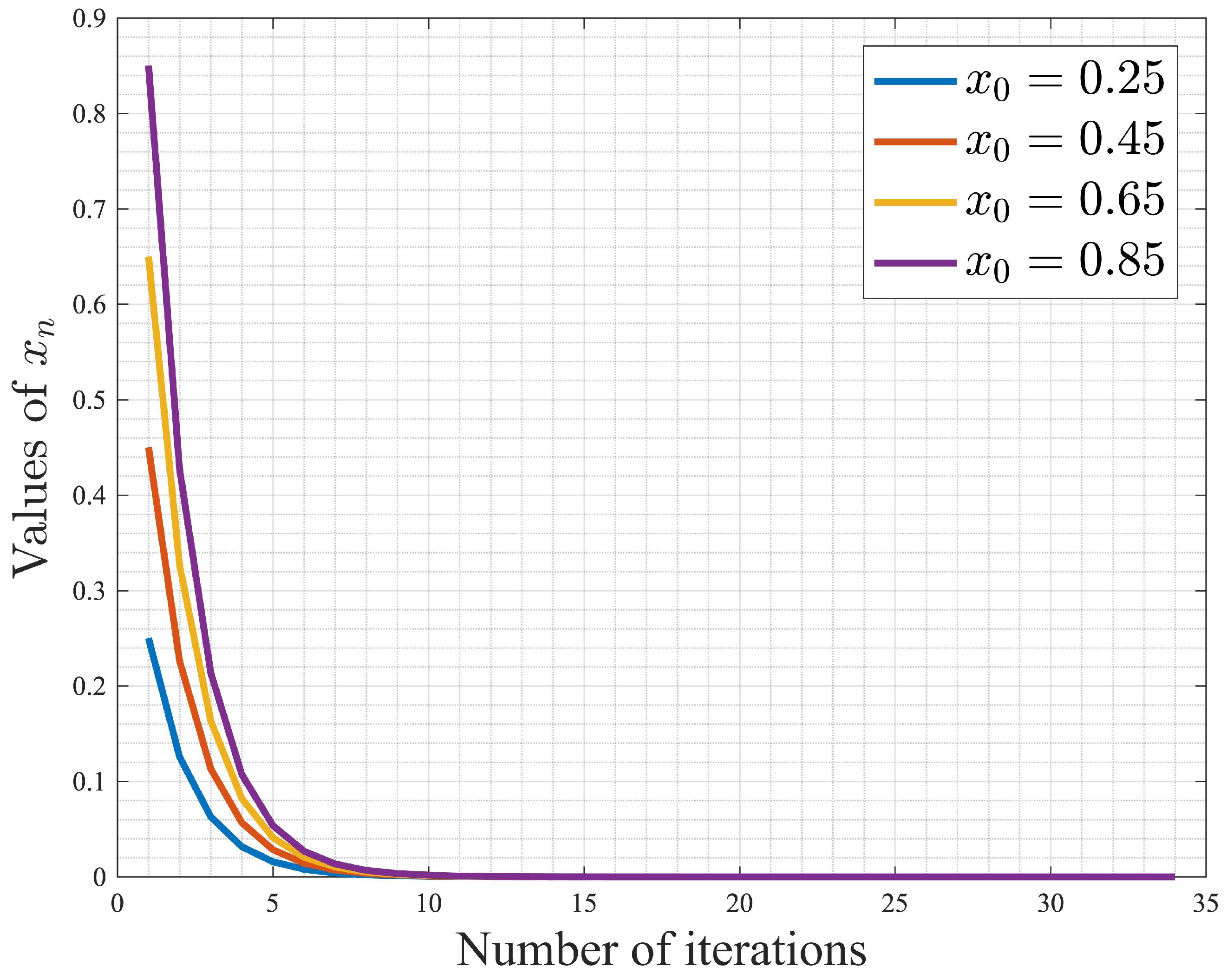
5.4. Numerical Experiments

Example 1.

Let $C=[0,1]$ be a subset of a real Hilbert space $\mathbb{R}$ with the usual inner product $\langle ·,·\rangle$ and define the mappings $S,T,F,\varphi :C\to C$ by

$$S\left(x\right)={\displaystyle \frac{x}{3}},T\left(x\right)={\displaystyle \frac{x}{2}},F\left(x\right)=2x,\mathrm{and}\varphi \left(x\right)={\displaystyle \frac{x}{4}}.$$

Let sequence $\left\{x_n\right\}$ be generated by algorithm (9), where ${\beta }_n=\frac{1}{10n+1},w_n=\frac{1}{20n+1},$${\lambda }_n=\frac{1}{30n+1},\mu =\frac{1}{4}$ and $\gamma =\frac{1}{4}$ Then, sequence $\left\{x_n\right\}$ converges strongly to $0.$

Under the different setting of initial points $x_0=0.25,0.45,0.65,0.85$, the computational results of algorithm (9) are given in both

Table 1. The approximation value via the algorithm (9) in the initial point $x_0$.

Iterate	${\mathit{x}}_0=0.25$	${\mathit{x}}_0=0.45$	${\mathit{x}}_0=0.65$	${\mathit{x}}_0=0.85$
1	0.1255435730	0.2259784314	0.3264132898	0.4268481482
2	0.0629054853	0.1132298736	0.1635542618	0.2138786501
3	0.0314970836	0.0566947504	0.0818924172	0.1070900841
4	0.0157651322	0.0283772379	0.0409893436	0.0536014494
5	0.0078891945	0.0142005501	0.0205119057	0.0268232613
6	0.0039473573	0.0071052432	0.0102631290	0.0134210149
7	0.0019748611	0.0035547500	0.0051346389	0.0067145278
8	0.0009879478	0.0017783060	0.0025686642	0.0033590224
9	0.0004942037	0.0008895667	0.0012849297	0.0016802927
10	0.0002472053	0.0004449695	0.0006427338	0.0008404980
11	0.0001236497	0.0002225694	0.0003214891	0.0004204088
12	0.0000618464	0.0001113235	0.0001608006	0.0002102777
13	0.0000309331	0.0000556796	0.0000804262	0.0001051727
14	0.0000154712	0.0000278481	0.0000402251	0.0000526020
15	0.0000077377	0.0000139279	0.0000201181	0.0000263083
16	0.0000038699	0.0000069658	0.0000100617	0.0000131576
17	0.0000019354	0.0000034838	0.0000050321	0.0000065804
18	0.0000009679	0.0000017423	0.0000025166	0.0000032910
19	0.0000004841	0.0000008713	0.0000012586	0.0000016458
20	0.0000002421	0.0000004358	0.0000006294	0.0000008231
21	0.0000001211	0.0000002179	0.0000003148	0.0000004116
22	0.0000000605	0.0000001090	0.0000001574	0.0000002059
23	0.0000000303	0.0000000545	0.0000000787	0.0000001029
24	0.0000000151	0.0000000273	0.0000000394	0.0000000515
25	0.0000000076	0.0000000136	0.0000000197	0.0000000257
26	0.0000000038	0.0000000068	0.0000000098	0.0000000129
27	0.0000000019	0.0000000034	0.0000000049	0.0000000064
28	0.0000000009	0.0000000017	0.0000000025	0.0000000032
29	0.0000000005	0.0000000009	0.0000000012	0.0000000016
30	0.0000000002	0.0000000004	0.0000000006	0.0000000008
31	0.0000000001	0.0000000002	0.0000000003	0.0000000004
32	0.0000000001	0.0000000001	0.0000000002	0.0000000002
33	0.0000000001	0.0000000001	0.0000000001	0.0000000001
34	0.0000000001	0.0000000001	0.0000000001	0.0000000001

and Figure 1.

6. Conclusions

According to the importance and attractiveness of hierarchical problems, in our research, we applied the viscosity technique together with a generalized implicit double midpoint rule to find a fixed point of nonexpansive mapping in the framework of real Hilbert spaces. We obtain the strong convergence theorem of our designed algorithm which can solve fixed point problem and also it is the same solution of our mentioned hierarchical problem. We also we propose the deduced corollaries and express how to apply our algorithm to solve other problems including the nonlinear Fredholm integral equation, convex minimization problem and hierarchical minimization. Moreover, we conduct a numerical experiment under a different initial point to illustrate the effectiveness of our algorithm.

References

1. Hartman, P.; Stampacchia, G. On some nonlinear elliptic differential functional equations. Acta Math. 1966, 115, 271–310. [Google Scholar] [CrossRef]
2. Kirk, W.A. Fixed point theorem for mappings which do not increase distance. Am. Math. Mon. 1965, 72, 1004–1006. [Google Scholar] [CrossRef] [Green Version]
3. Combettes, P.L. A block-itrative surrogate constraint splitting method for quadratic signal recovery. IEEE Trans. Signal Process. 2003, 51, 1771–1782. [Google Scholar] [CrossRef] [Green Version]
4. Gu, G.; Wang, S.; Cho, Y.J. Strong convergence algorithms for hierarchical fixed points problems and variational inequalities. J. Appl. Math. 2011, 2011, 164978. [Google Scholar] [CrossRef] [Green Version]
5. Hirstoaga, S.A. Iterative selection method for common fixed point problems. J. Math. Anal. Appl. 2006, 324, 1020–1035. [Google Scholar] [CrossRef] [Green Version]
6. Iiduka, H.; Yamada, I. A subgradient-type method for the equilibrium problem over the fixed point set and its applications. Optimization 2009, 58, 251–261. [Google Scholar] [CrossRef]
7. Marino, G.; Xu, H.K. Explicit hierarchical fixed point approach to variational inequalities. J. Optim. Theory Appl. 2011, 149, 61–78. [Google Scholar] [CrossRef]
8. Pakdeerat, N.; Sitthithakerngkiet, K. Approximating methods for monotone inclusion and two variational inequality. Bangmod Int. J. Math. Comp. Sci. 2020, 6, 71–89. [Google Scholar]
9. Slavakis, K.; Yamada, I. Robust wideband beamforming by the hybrid steepest descent method. J. Math. Anal. Appl. 2007, 55, 4511–4522. [Google Scholar] [CrossRef]
10. Slavakis, K.; Yamada, I.; Sakaniwa, K. Computation of symmetric positive definite Toeplitz matrices by the hybrid steepest descent method. Signal Process 2003, 83, 1135–1140. [Google Scholar] [CrossRef]
11. Yamada, I. The hybrid steepest descent method for the variational inequality problems over the intersection of fixed point sets of nonexpansive mappings. Inherently Parallel Algorithms Feasibility Optim. Their Appl. 2001, 8, 473–504. [Google Scholar]
12. Yao, Y.; Cho, J.; Liou, Y.C. Iterative algorithms for hierarcical fixed points problems and variational inequalities. Math. Comput. Model. 2010, 52, 1697–1705. [Google Scholar] [CrossRef]
13. Yao, Y.; Cho, J.; Liou, Y.C. Hierarchical convergence of an implicit double net algorithm for nonexpansive semigroups and variational inequality problems. Fixed Point Theory Appl. 2011, 2011, 101. [Google Scholar] [CrossRef] [Green Version]
14. Yao, Y.; Cho, Y.J.; Yang, P.X. An iterative algorithm for a hierarchical problem. J. Appl. Math. 2012, 2012, 320421. [Google Scholar] [CrossRef] [Green Version]
15. Yao, Y.; Liou, Y.C.; Chen, C.P. Hierarchical convergence of a double-net algorithm for equilibrium problems and variational inequality problems. Fixed Point Theory Appl. 2010, 2010, 642584. [Google Scholar] [CrossRef] [Green Version]
16. Yamada, I.; Ogura, N. Hybrid steepest descent method for variational inequality problem over the fixed point set of certain quasi-nonexpansive mapping. Numer. Funct. Anal. Optim. 2004, 25, 619–655. [Google Scholar] [CrossRef]
17. Yamada, I.; Ogura, N.; Shirakawa, N. A numerically robust hybrid steepest descent method for the convexly constrained generalized inverse problems. Am. Math. Soc. 2002, 313, 269–305. [Google Scholar]
18. Yao, Y.; Liou, Y.C.; Kang, S.M. Algorithms construction for variational inequaliies. Fixed Point Theory Appl. 2011, 2011, 794203. [Google Scholar] [CrossRef] [Green Version]
19. Ceng, L.C.; Ansari, Q.H.; Yao, J.C. Iterative methods for triple hierarchical variational inequalities in Hilbert spaces. J. Optim. Theory Appl. 2011, 151, 489–512. [Google Scholar] [CrossRef]
20. Kumam, P.; Jitpeera, T. Strong convergence of an iterative algorithm for hierarchical problems. Abstract Appl. Anal. 2014, 2014, 678147. [Google Scholar] [CrossRef] [Green Version]
21. Alghamdi, M.A.; Alghamadi, M.A.; Shahzad, N.; Xu, H.K. The implicit midpoint rule for nonexpansive mappings. Fixed Point Theory Appl. 2014, 2014, 96. [Google Scholar] [CrossRef] [Green Version]
22. Xu, H.K.; Alghamdi, M.A.; Shahzad, N. The viscosity technique for the implicit midpoint rule of nonexpansive mappings in Hilbert spaces. Fixed Point Theory Appl. 2015, 2015, 41. [Google Scholar] [CrossRef] [Green Version]
23. Dhakal, S.; Sintunavarat, W. The viscosity method for the implicit double midpoint rule with numerical results and its applications. Comput. Appl. Math. 2019, 38, 40. [Google Scholar] [CrossRef]
24. Xu, H.K. Iterative algorithms for nonlinear operators. J. Lond. Math. Soc. 2002, 66, 240–256. [Google Scholar] [CrossRef]
25. Goebel, K.; Kirk, W.A. Topics in Metric Fixed Point; Cambridge University Press: Cambridge, UK, 1990; Volume 28. [Google Scholar]
26. Nieto, J.J.; Xu, H.K. Solvability of nonlinear Volterra and Fredholm equations in weighted spaces. Nonlinear Anal. 1995, 24, 1289–1297. [Google Scholar] [CrossRef]
27. Cabot, A. Proximal point algorithm controlled by a slowly vanishing term: Applications to hierarchical minimization. SIAM J. Optim. 2005, 15, 555–572. [Google Scholar] [CrossRef]
Figure 1. Values of x n .
Mathematics 10 04755 g001