Reduce-Order Modeling and Higher Order Numerical Solutions for Unsteady Flow and Heat Transfer in Boundary Layer with Internal Heating

Abstract

We obtain similarity transformations to reduce a system of partial differential equations representing the unsteady fluid flow and heat transfer in a boundary layer with heat generation/absorption using Lie symmetry algebra. There exist seven Lie symmetries for this system of differential equations having three independent and three dependent variables. We use these Lie symmetries for the reduced-order modeling of the flow equations by constructing invariants corresponding to linear combinations of these Lie point symmetries. This procedure reduces one independent variable of the concerned fluid flow model when applied once. Double reductions are achieved by employing invariants twice that lead to ordinary differential equations with one independent and two dependent variables. Similarity transformations are constructed using these two sets of derived invariants corresponding to linear combinations of the Lie point symmetries. These similarity transformations have not been obtained earlier for this flow model. Moreover, the corresponding reduced systems of ordinary differential equations are different from those which exist in the literature for fluid flow and heat transfer that we have been dealing with. We obtain multiple similarity transformations which lead us to new classes of systems of ordinary differential equations. Accurate numerical solutions of these systems are obtained using the combination of an adaptive fourth-order Runge–Kutta method and shooting procedure. Effects of variation of unsteadiness parameter, Prandtl number and heat generation/absorption on fluid velocity, skin friction, surface temperature and heat flux are studied and presented with the help of tables and figures.

1. Introduction

With the advancements in industrial manufacturing processes, the accurate prediction of flow and heat transfer is of prime importance. Many industrial and food processes involve heat transfer in thin film flow, e.g., polymer coatings, metal sheets extractions, wire coatings, heat exchangers, reactor fluidization, surface paint processing, etc. In most of these processes, the surface finish, thickness and quality of coatings depend on the fluid flow and heat transfer in the boundary layer/thin films. Moreover, in numerous applications, fluid flow and heat transfer in the boundary layer involve heat generation/absorption effects, such as electric kettles, air conditioning, aerodynamic heating, solar water heaters, cooling in electronic devices using heat sinks, and temperature control techniques in the stacks of batteries. In many of these applications, the heat transfer rate and fluid velocity changes with time, thereby making the behavior of the problem unsteady.

The unsteady boundary layer flows involving heat transfer are modeled using Navier–Stokes equations. Normally, their solution could only be possible using numerical integration [1] due to the non-existence of the exact solutions in most of the cases for such nonlinear equations. However, if we restrict the motion of fluid to a specific group of coordinates and time dependence, we can derive similarity transformations to map flow equations into their simpler and analytically solvable forms. By using similarity transformations, the system of partial differential equations (PDEs) representing the unsteady fluid and heat transfer in the boundary layer flow is mapped into a system of coupled nonlinear ordinary differential equations (ODEs). Such reductions fall into the category of reduced-order modeling. Reduced-order modeling is a mathematical procedure that reduces the computational complexity of the concerned systems. The similarity transformations provide reductions of the dependent and independent variables of the fluid flow model, which brings down the computational complexity of these models. Numerous exact, analytic or/and approximate solution techniques for these systems of ODEs are available as compared to system PDEs for fluid flow and heat transfer in thin films.

In [2], the idea of [3] is implemented to model the unsteady fluid flow in thin film and [4] incorporated the heat transfer effects in it. Many researchers have studied these flow and heat transfer models [5,6,7,8,9,10,11,12,13,14,15] using a few similarity transformations. These studies have been conducted under multiple physical conditions, e.g., unsteady heat transfer in non-Newtonian fluid using power-law, fluid flow in an unsteady sheet by integrating thermocapillarity effects, fluid flow in an unsteady sheet by incorporating thermocapillarity effects with variable fluid properties, MHD flow with heat transfer in an unsteady stretching sheet with a non-uniform heat source, heat transfer with viscous dissipation on an unsteady stretching sheet, fluid flow and heat transfer on an unsteady surface with thermocapillarity and radiation effects, fluid flow and heat transfer on an unsteady stretching surface in the presence of radiation and with variable fluid properties, heat transfer in nanofluid thin film on an unsteady stretching sheet, etc. The reductions in the above cited works through similarity transformations are valid for a specific time interval. An extensive numerical and analytic treatment of flow in thin films has been completed to present optimum flow and heat transfer to acquire the desired refinements of many industrial products depending on such flows.

The Lie symmetry method is a mathematical technique by which one obtains similarity reductions for differential equations (DEs) if there exist Lie point symmetries [16,17,18] for these DEs. Previously, researchers used Lie point symmetries to derive similarity transformations for differential equations [19,20,21,22,23,24,25,26,27,28], e.g., for modified 1D shallow-water equations, the spatial motion on a rotating plane of incompressible fluid on shallow water, free convective nanofluid flow with heat generation/absorption on a chemically reacting sheet in porous medium, the Green Naghdi model hyperbolic and shallow water equations, a Schwartzian $(2+1)$-dimensional wave equation with a variable coefficient for shallow water, rotating shallow water equations, 2D shallow water equations in Lagrangian coordinates with a constant Coriolis parameter, a family of $1+1$ 5th-order PDEs, unsteady boundary layer flow on a vertical sheet with free convection and shallow water equations with Coriolis force, etc. However, in most of these studies, either single reduction is made, or double reduction is completed using general boundary conditions.

In this study, we derive Lie symmetries for heat transfer and fluid flow in an unsteady stretching sheet in the presence of heat generation/absorption. These Lie point symmetries may reduce the dependent and/or independent variables of flow equations considered through functions that remain invariant under Lie symmetry generators that are called invariants. In these flow equations, we have three independent and three dependent variables subject to specific boundary conditions. Using invariants associated with linear combinations of derived symmetries that is again a Lie symmetry, we reduce the PDEs of the flow and heat transfer into systems of equations with two independent and three dependent variables. Repeating the same procedure on these first reductions of PDEs, i.e., we obtain Lie symmetries of these systems, and using invariants corresponding to the obtained symmetries, we provide another reduction which finally leads to systems of ODEs. By combining invariants employed in these two reductions, we construct similarity transformations. These similarity transformations can map the flow equations straight to ODEs; for a detailed procedure, the reader is referred to [29]. A similar study is conducted by [30], using a similarity transformation of the form employed by, e.g., [2,4]. These are different from those presented here. Hence, the systems of ODEs deduced by using them and the ranges in which these similarity transformations are applicable are also different from those imposed in [30]. Moreover, we present the velocity and heat profiles in those ranges of the parameters involved, which either have not been considered earlier or solutions have not been approximated there.

In Section 2, the mathematical formulation of the flow, construction of Lie symmetries, invariants, similarity transformations and reductions to ODEs of the flow equations are presented. Section 3 discusses the numerical solution procedure. In Section 4, we have presented the results, which are followed by the conclusions.

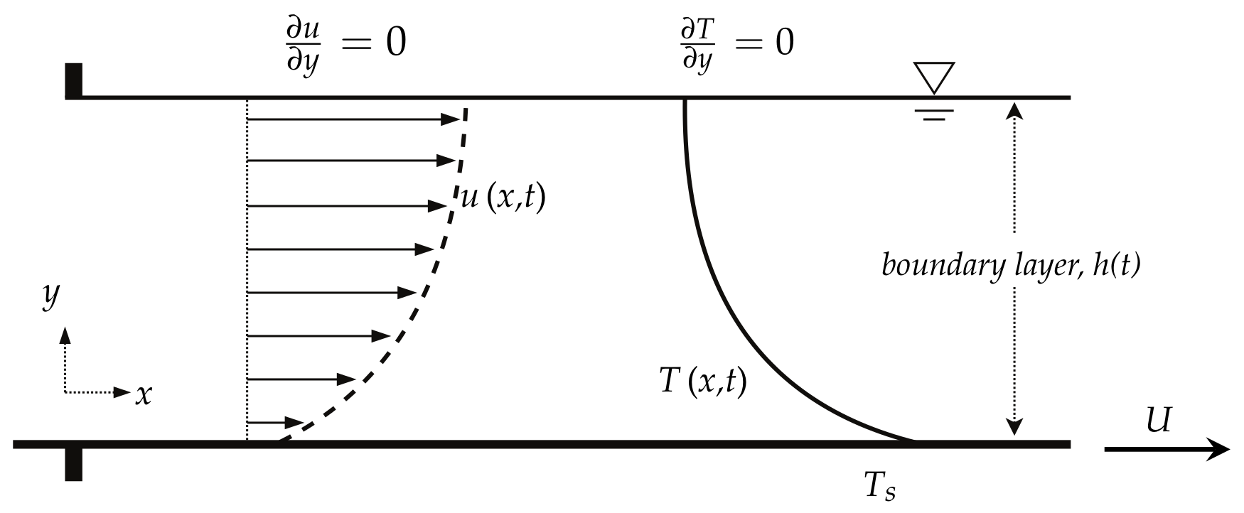
2. Mathematical Formulation, Lie Symmetries, Similarity Transformations and Reductions of Flow Equations

An incompressible, viscous, laminar and unsteady fluid coming out of origin of the coordinate system on a thin horizontal surface along with the heat transfer is considered here, as shown in Figure 1. In addition to that, it is also assumed that the temperature variations are small, and thus, the viscosity of fluid remains constant. The pressure and gravitational effects are also negligible. Initially, the temperature and velocity are taken as arbitrary functions of x-coordinate and time t. It is further assumed that the flow is free from any kind of surface waves, and streamwise diffusion is negligible. Under the stated assumptions, the governing 2D boundary layer equations with uniform heat generation/absorption are written as

$$\begin{array}{cc}\hfill & \frac{\partial u}{\partial x}+\frac{\partial v}{\partial y}=0,\hfill \\ \hfill & \frac{\partial u}{\partial t}+u\frac{\partial u}{\partial x}+v\frac{\partial u}{\partial y}=\nu \left(\frac{{\partial }^{2}u}{\partial y^2}\right),\hfill \\ \hfill & \rho C_p\left(\frac{\partial T}{\partial t}+u\frac{\partial T}{\partial x}+v\frac{\partial T}{\partial y}\right)=\kappa \left(\frac{{\partial }^{2}T}{\partial y^2}+\mathit{H}\right),\hfill \end{array}$$

(1)

subject to

$$\begin{array}{cc}\hfill & \mathrm{at}y=0:u=U,v=0,T=T_s,\hfill \\ \hfill & \mathrm{at}y=h\left(t\right):v=\frac{dh}{dt},\frac{\partial u}{\partial y}=\frac{\partial T}{\partial y}=0.\hfill \end{array}$$

(2)

In (1) and (2) x, y are the coordinates parallel and normal to the stretching surface and u, v are the velocities in these directions, respectively. T is the temperature, t is the time, $\rho$ is the density, $\nu$ is the kinematic viscosity, $C_p$ is the specific heat at constant pressure, $\kappa$ is the thermal diffusivity and H is the heat generation/absorption per unit volume and is defined as

$$\begin{array}{cc}\hfill & \mathit{H}=\left(\frac{\tilde{U}\left(T-T_0\right)}{x\nu }\right)G^{*},\hfill \end{array}$$

(3)

where $\tilde{U}$ is considered as velocity in the x-direction due to the flow in [30], which implies

$$\begin{array}{cc}\hfill & \tilde{U}=U=\frac{bx}{\left(1-at\right)}.\hfill \end{array}$$

(4)

In (3), $T_0$ is temperature at the origin and $G^{*}$ is the temperature-dependent heat generation/absorption parameter [30]. After simplifying, H is observed to be a function of temperature, $t^{-1}$ and $G^{*}$. For heat addition, $G^{*}>0$, and for heat absorption, $G^{*}<0$. By restricting the motion in its own horizontal plane and imposing specific time dependence, the surface velocity U and temperature $T_s$ in [30] are written as (4) and

$$\begin{array}{cc}\hfill & T_s=T_0-\left(\frac{d{x}^{r_1}}{\nu }\right)T_{ref}{(1-at)}^{-r_2},\hfill \end{array}$$

(5)

respectively, where $T_{ref}$ is a reference temperature, $r_1$ and $r_2$ are positive constants and d is a positive proportionality constant with dimension length${}^{2-r}$time${}^{-1}$ [9]. A similarity transformation that is compatible with (4) and (5) is

$$\begin{array}{cc}\hfill & \eta =\frac{y}{\beta }\sqrt{\frac{b}{\nu \left(1-at\right)}},u=\frac{bx}{\left(1-at\right)}{f}^{\prime }\left(\eta \right),v=-\sqrt{\frac{b\nu }{\left(1-at\right)}}\beta f\left(\eta \right),\hfill \\ \hfill & T=T_0-\left(\frac{d{x}^{r_1}}{\nu }\right)T_{ref}{(1-at)}^{-r_2}\vartheta \left(\eta \right),\hfill \end{array}$$

(6)

where a and b are positive constants and have the dimensions of $t^{-1}$. $\beta$ is the dimensionless boundary layer/film thickness, f is the stream function, $\vartheta$ is the dimensionless temperature and $\eta$ is the similarity variable. Aziz et al. [30] employed these transformations on (1) and obtained the system of ODEs as

$$\begin{array}{cc}\hfill & f^{‴}+\lambda \left(f{f}^{″}-S(f^{\prime }+\frac{\eta }{2}{f}^{″})-{f^{\prime }}^2\right)=0,\hfill \\ \hfill & \frac{{\vartheta }^{″}}{Pr}+\lambda \left(f{\vartheta }^{\prime }-r_1{f}^{\prime }\vartheta -S(\frac{\eta }{2}{\vartheta }^{\prime }+r_{2}S\vartheta )+\frac{1}{Pr}{G}^{*}\vartheta \right)=0.\hfill \end{array}$$

(7)

Likewise, considering (4) and (5) in (2) and transforming them via (6), we obtain

$$\begin{array}{cc}\hfill & at\eta =0:f=0,f^{\prime }=1,\vartheta =1,\hfill \\ \hfill & at\eta =1:f^{″}=0,{\vartheta }^{\prime }=0,f=\frac{1}{2}S,\hfill \end{array}$$

(8)

where prime denotes the derivative with respect to $\eta$, $S=a/b$ denotes the dimensionless unsteadiness parameter, $Pr=\frac{\rho \nu C_p}{\kappa }$ is the Prandtl number and $\lambda ={\beta }^2$ is the dimensionless film thickness. It is important to note that the above similarity transformations are valid only for $t<a^{-1}$. In the subsequent sections, we are performing reduced-order modeling using Lie symmetry algebra.

2.1. Lie Symmetries and Invariants

To derive similarity transformations for the system of PDEs (1), we first obtain Lie point symmetry generators for this system that is a vector field as

$$\begin{array}{cc}\hfill & \mathbf{X}={\xi }_i\frac{\partial }{\partial {\psi }_i}+{\varphi }_i\frac{\partial }{\partial {\zeta }_i},\hfill \end{array}$$

(9)

where $i=1,2,3$, $\xi$ and $\varphi$ are infinitesimal coordinates and they are functions of independent $x,y,t$ and dependent variables $u,v,T$, respectively. The system (1) and boundary conditions (2) contain both first and second-order partial derivatives. For this, we require first and second extensions of (9) to operate on them. MAPLE contains an algebraic procedure to derive Lie point symmetries for DEs; here, we use it to obtain Lie point symmetries of system (1). In (3), we consider $\tilde{U}=\frac{bx}{at}$, that is different from $U(t,x)$, given in conditions (2) which provides

$$\begin{array}{cc}\hfill & H=\frac{b}{a\nu t}{G}^{*}(T-T_0).\hfill \end{array}$$

(10)

The stretchable sheet velocity $U(t,x)$, is obtained in the subsequent section by applying the Lie symmetry generators. Hence, it is not expected to be similar for all symmetries that are derived using (10) in system (1). System (1) admits an infinite dimensional Lie point symmetry algebra that is spanned by the following symmetry generators

$$\begin{array}{cc}\hfill & {\mathbf{X}}_{\mathbf{1}}^{{}^{\infty }}=\frac{\partial }{\partial x}+f_1(t,x)\frac{\partial }{\partial y}+(f_{1,t}+u{f}_{1,x})\frac{\partial }{\partial v},\hfill \\ \hfill & {\mathbf{X}}_{\mathbf{2}}^{{}^{\infty }}=t\frac{\partial }{\partial x}+f_2(t,x)\frac{\partial }{\partial y}+\frac{\partial }{\partial u}+(f_{2,t}+u{f}_{2,x})\frac{\partial }{\partial v},\hfill \\ \hfill & {\mathbf{X}}_{\mathbf{3}}^{{}^{\infty }}=x\frac{\partial }{\partial x}+f_3(t,x)\frac{\partial }{\partial y}+u\frac{\partial }{\partial u}+(f_{3,t}+u{f}_{3,x})\frac{\partial }{\partial v},\hfill \\ \hfill & {\mathbf{X}}_{\mathbf{4}}^{{}^{\infty }}=f_4(t,x)\frac{\partial }{\partial y}+(T-T_0)\frac{\partial }{\partial T}+(f_{4,t}+u{f}_{4,x})\frac{\partial }{\partial v},\hfill \\ \hfill & {\mathbf{X}}_{\mathbf{5}}^{{}^{\infty }}=t\frac{\partial }{\partial t}+(\frac{y}{2}+f_5(t,x))\frac{\partial }{\partial y}-u\frac{\partial }{\partial u}+(f_{5,t}+u{f}_{5,x}-\frac{v}{2})\frac{\partial }{\partial v},\hfill \\ \hfill & {\mathbf{X}}_{\mathbf{6}}^{{}^{\infty }}=f_6(t,x)\frac{\partial }{\partial y}+t^{\frac{b\kappa G^{*}}{a{C}_p\rho \nu }}\frac{\partial }{\partial T}+(f_{6,t}+u{f}_{6,x})\frac{\partial }{\partial v},\hfill \\ \hfill & {\mathbf{X}}_{\mathbf{7}}^{{}^{\infty }}=\frac{\partial }{\partial t}+f_7(t,x)\frac{\partial }{\partial y}+\frac{(T-T_0)b\kappa G^{*}}{a{C}_p\rho \nu t}\frac{\partial }{\partial T}+(f_{7,t}+u{f}_{7,x})\frac{\partial }{\partial v},\hfill \\ \hfill & {\mathbf{X}}_{\mathbf{8}}^{{}^{\infty }}=f_8(t,x)\frac{\partial }{\partial y}+(f_{8,t}+u{f}_{8,x})\frac{\partial }{\partial v}.\hfill \end{array}$$

(11)

By considering $f_i(t,x)=0,$ for $i=1,2,\dots ,8$, we obtain a finite dimensional algebra. The reason to use finite dimensional algebra is to extract scaling transformations to perform the reduced-order modeling. Scaling transformations are the most suitable mappings that are employed for reduction of the independent variables of the flow models.

Table 1. Lie point symmetry generators and invariants.

Symmetry	Invariants-Conserved Quantities
${\mathbf{X}}_1=\frac{\partial }{\partial x}$	$x,y,T,u,v$
${\mathbf{X}}_2=t\frac{\partial }{\partial x}+\frac{\partial }{\partial u}$	$t,y,T,\frac{u}{x},v$
${\mathbf{X}}_3=x\frac{\partial }{\partial x}+u\frac{\partial }{\partial u}$	$t,y,T,\frac{u}{x},v$
${\mathbf{X}}_4=\left(T-T_0\right)\frac{\partial }{\partial T}$	$t,x,y,u,v$
${\mathbf{X}}_5=t\frac{\partial }{\partial t}+\frac{y}{2}\frac{\partial }{\partial y}-u\frac{\partial }{\partial u}-\frac{v}{2}\frac{\partial }{\partial v}$	$x,\frac{y}{t},T,ut,v$
${\mathbf{X}}_6=\left(t^{\frac{b\kappa G^{*}}{a{C}_p\rho \nu }}\right)\frac{\partial }{\partial T}$	$t,x,y,u,v$
${\mathbf{X}}_7=\frac{\partial }{\partial t}+\frac{b(T-T_0)\kappa G*}{a{C}_p\rho \nu t}\frac{\partial }{\partial T}$	$x,y,\frac{T-T_0}{t},u,v$

presents the finite dimensional symmetry algebra and corresponding invariants for system (1). These symmetry generators ${\mathbf{X}}_1,\dots ,{\mathbf{X}}_7$ and their linear combinations leave system (1) and associated conditions invariant. The boundary conditions (2) also remain invariant under these generators. Both U and T at $y=0$ are functions of x-coordinate and time t. There, invariant forms under ${\mathbf{X}}_1,\dots ,{\mathbf{X}}_7$ are determined by applying these generators on them and evaluating the resulting expressions on these conditions. However, when a single symmetry is used in this procedure, both U and T become either functions of x or t. In this work, we want to keep them functions of both x and t. We achieved it through linear combinations of the symmetry generators ${\mathbf{X}}_1,\dots ,{\mathbf{X}}_7$ by adding two at a time, which also leave boundary conditions (2) invariant. We obtain seven such combinations in which these conditions remain functions of both space and time, as shown in

Table 2. First invariants for similarity transformations.

Case	Symmetry and Invariants	Corresponding Boundary Conditions
1	X${}_3$ + X${}_4$
	$\begin{array}{c}t,y,\frac{u}{x},v,\frac{T-T_0}{x}\hfill \end{array}$	$\begin{array}{c}aty=0:v=0,u=x\overline{U}\left(t\right),T=T_0+x{\overline{T}}_s\left(t\right)\hfill \\ aty=h\left(t\right):v=\frac{\partial h}{\partial t},\frac{\partial u}{\partial y}=\frac{\partial T}{\partial y}=0\hfill \end{array}$
2	X${}_2$ + X${}_5$
	$\begin{array}{c}x-t,\frac{y}{\sqrt{t}},ut-t,\sqrt{t}v,T\hfill \end{array}$	$\begin{array}{c}aty=0:v=0,u=1+\frac{\overline{U}(x-t)}{t},T={\overline{T}}_s(x-t)\hfill \\ aty=a_3\sqrt{t}:v=\frac{a_3}{2\sqrt{t}},\frac{\partial u}{\partial y}=\frac{\partial T}{\partial y}=0\hfill \end{array}$
3	X${}_3$ + X${}_5$
	$\begin{array}{c}\frac{x}{t},\frac{y}{\sqrt{t}},u,\sqrt{t}v,T\hfill \end{array}$	$\begin{array}{c}aty=0:v=0,u=\overline{U}\left(\frac{x}{t}\right),T={\overline{T}}_s\left(\frac{x}{t}\right)\hfill \\ aty=a_3\sqrt{t}:v=\frac{a_3}{2\sqrt{t}},\frac{\partial u}{\partial y}=\frac{\partial T}{\partial y}=0\hfill \end{array}$
4	X${}_3$ + X${}_6$
	$\begin{array}{c}t,y,\frac{u}{x},v,T-ln\left(x\right)\left(t^{\frac{b\kappa G^{*}}{a{C}_p\rho \nu }}\right)\hfill \end{array}$	$\begin{array}{c}aty=0:v=0,u=x\overline{U}\left(t\right),T={\overline{T}}_s\left(t\right)+ln\left(x\right)t^{\frac{b\kappa G^{*}}{a{C}_p\rho \nu }}\hfill \\ aty=h\left(t\right):v=\frac{\partial h}{\partial t},\frac{\partial u}{\partial y}=\frac{\partial T}{\partial y}=0\hfill \end{array}$
5	X${}_4$ + X${}_5$
	$\begin{array}{c}x,\frac{y}{\sqrt{t}},tu,\sqrt{t}v,\frac{T-T_0}{t}\hfill \end{array}$	$\begin{array}{c}aty=0:v=0,u=\frac{\overline{U}\left(x\right)}{t},T=T_0+t{\overline{T}}_s\left(x\right)\hfill \\ aty=a_3\sqrt{t}:v=\frac{a_3}{2\sqrt{t}},\frac{\partial u}{\partial y}=\frac{\partial T}{\partial y}=0\hfill \end{array}$
6	X${}_5$ + X${}_6$
	$\begin{array}{c}x,\frac{y}{\sqrt{t}},tu,\sqrt{t}v,T-\frac{a{C}_p\rho \nu }{b\kappa G^{*}}{t}^{\frac{b\kappa G^{*}}{a{C}_p\rho \nu }}\hfill \end{array}$	$\begin{array}{c}aty=0:v=0,u=\frac{\overline{U}\left(x\right)}{t},T=\frac{a{C}_p\rho \nu }{b\kappa G^{*}}{t}^{\frac{b\kappa G^{*}}{a{C}_p\rho \nu }}+{\overline{T}}_s\left(x\right)\hfill \\ aty=a_3\sqrt{t}:v=\frac{a_3}{2\sqrt{t}},\frac{\partial u}{\partial y}=\frac{\partial T}{\partial y}=0\hfill \end{array}$
7	X${}_5$ + X${}_7$
	$\begin{array}{c}x,\frac{y}{\sqrt{1+t}},u(t+1),\sqrt{1+t}v,\hfill \\ {(1+t)}^{\frac{b\kappa G^{*}}{a{C}_p\rho \nu }}(T-T_0)t^{-\frac{b\kappa G^{*}}{a{C}_p\rho \nu }}\hfill \end{array}$	$\begin{array}{c}aty=0:v=0,u=\frac{\overline{U}\left(x\right)}{t+1},T=T_0+{(1+t)}^{-\frac{b\kappa G^{*}}{a{C}_p\rho \nu }}{t}^{\frac{b\kappa G^{*}}{a{C}_p\rho \nu }}{\overline{T}}_s\left(x\right)\hfill \\ aty=a_3\sqrt{1+t}:v=\frac{a_3}{2\sqrt{1+t}},\frac{\partial u}{\partial y}=\frac{\partial T}{\partial y}=0\hfill \end{array}$

.

2.2. Double Reductions and Construction of Similarity Transformations

Similarity transformations are derived through double reductions of differential equations (DEs) using Lie point symmetry generators. Consider Case 1 in Table 2, which is ${\mathbf{X}}_3+{\mathbf{X}}_4$. Except for $u=U(t,x)$ and $T=T_s(t,x)$, it leaves all other boundary conditions (2) invariant. The conditions $u=U(t,x)$ and $T=T_s(t,x)$ when inserted in the invariance criterion read as

$$\begin{array}{cc}\hfill & [{\mathbf{X}}_{\mathbf{3}}+{\mathbf{X}}_{\mathbf{4}}](u-U(t,x)){|}_{u=U(t,x)}=0,\hfill \\ \hfill & [{\mathbf{X}}_{\mathbf{3}}+{\mathbf{X}}_{\mathbf{4}}](T-T_s(t,x)){|}_{T=T_s(t,x)}=0.\hfill \end{array}$$

(12)

Applying these symmetry generators and expanding the resulting expressions at $u=U(t,x)$ and $T=T_s(t,x)$ provides the following linear PDEs

$$\begin{array}{cc}\hfill & x\frac{\partial U(x,t)}{\partial x}-u=0,\hfill \\ \hfill & x\frac{\partial T_s(x,t)}{\partial x}-T+T_0=0.\hfill \end{array}$$

(13)

Solving these equations, we obtain

$$\begin{array}{cc}\hfill & u=x\overline{U}\left(t\right),\mathrm{and}T=T_0+x{\overline{T}}_s\left(t\right).\hfill \end{array}$$

(14)

Now, for the derivation of 0th-order differential invariants, we apply X${}_{{}_{34}}$ = X${}_3$ + X${}_4$, in the following invariance criterion

$$\begin{array}{cc}\hfill & {\mathbf{X}}_{{}_{\mathbf{34}}}J(t,x,y,u,v,T)=0,\hfill \end{array}$$

(15)

which leads to the following PDE

$$\begin{array}{cc}\hfill & x\frac{\partial J}{\partial x}+u\frac{\partial J}{\partial u}+\left(T-T_0\right)\frac{\partial J}{\partial T}=0.\hfill \end{array}$$

(16)

Solving it using MAPLE, we obtain five invariants {$t,y,\frac{u}{x},v,\frac{T-T_0}{x}$} with two independent $t,y$ and three dependent variables $\frac{u}{x},v,\frac{T-T_0}{x}$. We obtain first components of the claimed similarity transformations by renaming these invariants as follows

$$\begin{array}{cc}\hfill & c_1=t,c_2=y,P=\frac{u}{x},Q=v,R=\frac{T-T_0}{x}.\hfill \end{array}$$

(17)

This maps the system of PDEs (1) and conditions (2) to

$$\begin{array}{cc}\hfill & P+\frac{\partial Q}{\partial c_2}=0,\hfill \\ \hfill & \frac{\partial P}{\partial c_1}+P^2+Q\frac{\partial P}{\partial c_2}=\nu \left(\frac{{\partial }^{2}P}{\partial {c_2}^2}\right),\hfill \\ \hfill & \rho C_p\left(\frac{\partial R}{\partial c_1}+PR+Q\frac{\partial R}{\partial c_2}\right)=\kappa \left(\frac{{\partial }^{2}R}{\partial {c_2}^2}+\mathit{H}\right),\hfill \end{array}$$

(18)

and

$$\begin{array}{cc}\hfill & \mathrm{at}{c}_2=0:P=F\left(c_1\right),Q=0,R=G\left(c_1\right),\hfill \\ \hfill & \mathrm{at}{c}_2=h:Q=\frac{dh}{d{c}_1},\frac{\partial P}{\partial c_2}=\frac{\partial R}{\partial c_2}=0.\hfill \end{array}$$

(19)

For the second reduction, symmetry generators for system (18) are obtained that admits a $three$-dimensional Lie symmetry algebra

$$\begin{array}{cc}\hfill & {\mathbf{Y}}_{\mathbf{1}}=R\frac{\partial }{\partial R},{\mathbf{Y}}_{\mathbf{2}}=c_1\frac{\partial }{\partial c_1}+\frac{c_2}{2}\frac{\partial }{\partial c_2}-P\frac{\partial }{\partial P}-\frac{Q}{2}\frac{\partial }{\partial Q},\hfill \end{array}$$

$$\begin{array}{cc}\hfill & {\mathbf{Y}}_{\mathbf{3}}=\frac{\partial }{\partial c_1}+\left(\frac{bR\kappa G*}{a{C}_p{c}_1\rho \nu }\right)\frac{\partial }{\partial R}.\hfill \end{array}$$

(20)

The combination ${\mathbf{Y}}_1+{\mathbf{Y}}_2$ further converts the boundary conditions (19) to

$$\begin{array}{cc}\hfill & \mathrm{at}{c}_2=0:P=\frac{a_1}{c_1},Q=0,R=a_2{c}_1,\hfill \\ \hfill & \mathrm{at}{c}_2=a_3\sqrt{c_1}:Q=\frac{a_3}{2},\frac{\partial P}{\partial c_2}=\frac{\partial R}{\partial c_2}=0.\hfill \end{array}$$

(21)

The invariants obtained using these symmetries ${\mathbf{Y}}_1+{\mathbf{Y}}_2$ are {$\frac{c_2}{\sqrt{c_1}},P{c}_1,Q\sqrt{c_1},\frac{R}{c_1}$}, where now $\frac{c_2}{\sqrt{c_1}}$ is the new independent variable and $P{c}_1,Q\sqrt{c_1},\frac{R}{c_1}$ are the new dependent variables, which are given the following notations

$$\begin{array}{cc}\hfill & \chi =\frac{c_2}{\sqrt{c_1}},P{c}_1=L,Q\sqrt{c_1}=M,\frac{R}{c_1}=N.\hfill \end{array}$$

(22)

Using (22), the second reductions are performed that transform the system (18) and associated conditions (21) to

$$\begin{array}{cc}\hfill & L+M^{\prime }=0,\hfill \\ \hfill & L^2-L-\frac{\chi }{2}{L}^{\prime }+M{L}^{\prime }=\nu L^{″},\hfill \\ \hfill & LN+N-\frac{\chi }{2}{N}^{\prime }+M{N}^{\prime }=\frac{\kappa }{\rho C_p}{N}^{″}+\frac{b\kappa G^{*}N}{a\rho C_p\nu },\hfill \end{array}$$

(23)

and

$$\begin{array}{cc}\hfill & \mathrm{at}\chi =0:L=a_1,M=0,N=a_2,\hfill \\ \hfill & \mathrm{at}\chi =a_3:M=\frac{a_3}{2},L^{\prime }=N^{\prime }=0,\hfill \end{array}$$

(24)

where prime denotes differentiation with respect to $\chi$. In system (7), we have $Pr$, S and $\beta$. We introduce these variables in the similarity transformations constructed here by combining (17), (22) and

$$\begin{array}{cc}\hfill & \chi =\eta \beta \sqrt{\frac{a\nu }{b}},L=-\frac{b}{a}{f}^{\prime }\left(\eta \right),M=\beta \sqrt{\frac{b\nu }{a}}f\left(\eta \right),N=\vartheta \left(\eta \right),\hfill \end{array}$$

(25)

which leads to claimed similarity transformations

$$\begin{array}{cc}\hfill & u=-\frac{bx}{at}{f}^{\prime }\left(\eta \right),v=\beta \sqrt{\frac{b\nu }{at}}f\left(\eta \right),T=T_0+xt\vartheta \left(\eta \right),\eta =\frac{1}{\beta }\sqrt{\frac{b}{at\nu }}y.\hfill \end{array}$$

(26)

The set of similarity transformations (26) maps the system of PDEs (1) and boundary conditions (2) into system of ODEs as

$$\begin{array}{cc}\hfill & f^{‴}+\lambda \left(S{f}^{\prime }-f{f}^{″}+\frac{S\eta }{2}{f}^{″}+{f^{\prime }}^2\right)=0,\hfill \\ \hfill & \frac{1}{Pr}{\vartheta }^{″}+\lambda \left(-f{\vartheta }^{\prime }+\frac{S\eta }{2}{\vartheta }^{\prime }-S\vartheta +f^{\prime }\vartheta +\frac{1}{Pr}\vartheta G^{*}\right)=0,\hfill \end{array}$$

(27)

and

$$\begin{array}{cc}\hfill & at\eta =0:f=0,f^{\prime }=1,\vartheta =1,\hfill \\ \hfill & at\eta =1:f=\frac{1}{2}S,f^{″}=0,{\vartheta }^{\prime }=0.\hfill \end{array}$$

(28)

Using linear combinations of symmetries ${\mathbf{X}}_1-{\mathbf{X}}_7$, we perform double reductions and obtain a set of similarity transformations against each combination that reduces the system of PDEs (1) into systems of ODEs given in

Table 3. Similarity transformations and systems of ODEs.

Case	Symmetry Generator and Similarity Transformation	System of ODEs
1	X${}_3$ + X${}_4$
	$\begin{array}{c}v=\beta \sqrt{\frac{b\nu }{at}}f\left(\eta \right),u=-\frac{bx}{at}{f}^{\prime }\left(\eta \right)\hfill \\ \eta =\frac{1}{\beta }\sqrt{\frac{b}{at\nu }}y,T=T_0+xt\vartheta \left(\eta \right)\hfill \end{array}$	$\begin{array}{c}{f}^{‴}+\lambda \left(S{f}^{\prime }-f{f}^{″}+{f^{\prime }}^2+\frac{S\eta }{2}{f}^{″}\right)=0\hfill \\ \frac{1}{Pr}{\vartheta }^{″}+\lambda \left(-f{\vartheta }^{\prime }+\frac{S\eta }{2}{\vartheta }^{\prime }-S\vartheta +f^{\prime }\vartheta +\frac{1}{Pr}\vartheta G^{*}\right)=0\hfill \end{array}$
2	X${}_2$ + X${}_5$
	$\begin{array}{c}v=\beta \sqrt{\frac{b\nu }{at}}f\left(\eta \right),u=1-\frac{b(x-t)}{at}{f}^{\prime }\left(\eta \right)\hfill \\ \eta =\frac{1}{\beta }\sqrt{\frac{b}{at\nu }}y,T=T_0+(x-t)\vartheta \left(\eta \right)\hfill \end{array}$	$\begin{array}{c}{f}^{‴}+\lambda \left(S{f}^{\prime }-f{f}^{″}+{f^{\prime }}^2+\frac{S\eta }{2}{f}^{″}\right)=0\hfill \\ \frac{1}{Pr}{\vartheta }^{″}+\lambda \left(-f{\vartheta }^{\prime }+\frac{S\eta }{2}{\vartheta }^{\prime }+f^{\prime }\vartheta +\frac{1}{Pr}\vartheta G^{*}\right)=0\hfill \end{array}$
3	X${}_3$ + X${}_5$
	$\begin{array}{c}v=\beta \sqrt{\frac{b\nu }{at}}f\left(\eta \right),u=-\frac{bx}{at}{f}^{\prime }\left(\eta \right)\hfill \\ \eta =\frac{1}{\beta }\sqrt{\frac{b}{at\nu }}y,T=T_0+\frac{x}{t}\vartheta \left(\eta \right)\hfill \end{array}$	$\begin{array}{c}{f}^{‴}+\lambda \left(S{f}^{\prime }-f{f}^{″}+{f^{\prime }}^2+\frac{S\eta }{2}{f}^{″}\right)=0\hfill \\ \frac{1}{Pr}{\vartheta }^{″}+\lambda \left(-f{\vartheta }^{\prime }+\frac{S\eta }{2}{\vartheta }^{\prime }+S\vartheta +f^{\prime }\vartheta +\frac{1}{Pr}\vartheta G^{*}\right)=0\hfill \end{array}$
4	X${}_3$ + X${}_6$
	$\begin{array}{c}v=\beta \sqrt{\frac{b\nu }{at}}f\left(\eta \right),u=-\frac{bx}{at}{f}^{\prime }\left(\eta \right)\hfill \\ \eta =\frac{1}{\beta }\sqrt{\frac{b}{at\nu }}y,T=T_0+(\vartheta \left(\eta \right)+ln\left(x\right))t^{\frac{b\kappa G^{*}}{a{C}_p\rho \nu }}\hfill \end{array}$	$\begin{array}{c}{f}^{‴}+\lambda \left(S{f}^{\prime }-f{f}^{″}+{f^{\prime }}^2+\frac{S\eta }{2}{f}^{″}\right)=0\hfill \\ \frac{1}{Pr}{\vartheta }^{″}+\lambda \left(-f{\vartheta }^{\prime }+\frac{S\eta }{2}{\vartheta }^{\prime }+f^{\prime }\right)=0\hfill \end{array}$
5	X${}_4$ + X${}_5$
	$\begin{array}{c}v=\beta \sqrt{\frac{b\nu }{at}}f\left(\eta \right),u=-\frac{bx}{at}{f}^{\prime }\left(\eta \right)\hfill \\ \eta =\frac{1}{\beta }\sqrt{\frac{b}{at\nu }}y,T=T_0+xt\vartheta \left(\eta \right)\hfill \end{array}$	$\begin{array}{c}{f}^{‴}+\lambda \left(S{f}^{\prime }-f{f}^{″}+{f^{\prime }}^2+\frac{S\eta }{2}{f}^{″}\right)=0\hfill \\ \frac{1}{Pr}{\vartheta }^{″}+\lambda \left(-f{\vartheta }^{\prime }+\frac{S\eta }{2}{\vartheta }^{\prime }-S\vartheta +f^{\prime }\vartheta +\frac{1}{Pr}\vartheta G^{*}\right)=0\hfill \end{array}$
6	X${}_5$ + X${}_6$
	$\begin{array}{c}v=\beta \sqrt{\frac{b\nu }{at}}f\left(\eta \right),u=-\frac{bx}{at}{f}^{\prime }\left(\eta \right)\hfill \\ \eta =\frac{1}{\beta }\sqrt{\frac{b}{at\nu }}y,T=T_0+x\vartheta \left(\eta \right)+\frac{a{C}_p\rho \nu }{b\kappa G^{*}}{t}^{\frac{b\kappa G^{*}}{a{C}_p\rho \nu }}\hfill \end{array}$	$\begin{array}{c}{f}^{‴}+\lambda \left(S{f}^{\prime }-f{f}^{″}+{f^{\prime }}^2+\frac{S\eta }{2}{f}^{″}\right)=0\hfill \\ \frac{1}{Pr}{\vartheta }^{″}+\lambda \left(-f{\vartheta }^{\prime }+\frac{S\eta }{2}{\vartheta }^{\prime }+f^{\prime }\vartheta +\frac{1}{Pr}\vartheta G^{*}\right)=0\hfill \end{array}$
7	X${}_5$ + X${}_7$
	$\begin{array}{c}v=\beta \sqrt{\frac{b\nu }{a(1+t)}}f\left(\eta \right),u=-\frac{bx}{a(1+t)}{f}^{\prime }\left(\eta \right)\hfill \\ \eta =\frac{1}{\beta }\sqrt{\frac{b}{a\nu (1+t)}}y,T=T_0+x\vartheta \left(\eta \right){(1+t)}^{-\frac{b\kappa G^{*}}{a{C}_p\rho \nu }}{t}^{\frac{b\kappa G^{*}}{a{C}_p\rho \nu }}\hfill \end{array}$	$\begin{array}{c}{f}^{‴}+\lambda \left(S{f}^{\prime }-f{f}^{″}+{f^{\prime }}^2+\frac{S\eta }{2}{f}^{″}\right)=0\hfill \\ \frac{1}{Pr}{\vartheta }^{″}+\lambda \left(-f{\vartheta }^{\prime }+\frac{S\eta }{2}{\vartheta }^{\prime }+f^{\prime }\vartheta +\frac{1}{Pr}\vartheta G^{*}\right)=0\hfill \end{array}$

. The reason to consider only these linear combinations in Table 3 is the form of $U(t,x)$ and $T_s(t,x)$ they provide; i.e., both of them are functions of the x-coordinate and time-t in all cases. Once invariance of the conditions (2) under the admitted Lie point symmetries of the system (1) has been established, then it implies that any linear combination of these symmetries also leaves the associated conditions invariant.

The skin friction C_f and heat flux q_s are important physical parameters, and they are written as

$$\begin{array}{cc}\hfill & C_f=\left(\frac{2{\tau }_s}{\rho u^2}\right),\hfill \end{array}$$

(29)

$$\begin{array}{cc}\hfill & q_s=-\kappa {\left(\frac{\partial T}{\partial y}\right)}_{y=0},\hfill \end{array}$$

(30)

where ${\tau }_s$ is the shear stress

$$\begin{array}{cc}\hfill & {\tau }_s=\mu {\left(\frac{\partial u}{\partial y}\right)}_{y=0},\hfill \end{array}$$

(31)

Using the similarity transformations (26), i.e., for Case 1, we have

$$\begin{array}{cc}\hfill & C_f=\frac{2}{\beta \sqrt{R{e}_x}}{f}^{″}\left(0\right),\hfill \end{array}$$

(32)

$$\begin{array}{cc}\hfill & q_s=-\frac{x\kappa }{\beta \mu }\sqrt{\frac{b(1+x){\rho }^3}{a}}{\vartheta }^{\prime }\left(0\right),\hfill \end{array}$$

(33)

where $R{e}_x$ is the local Reynolds number.

3. Numerical Solutions

The solution of a nonlinear coupled system of ODEs, e.g., (7) subject to (8) is obtained by using the combination of most efficient Runge–Kutta Fehlberg numerical integration technique and shooting method. It is a fourth-order O(h${}^4$) accurate scheme with the fifth-order O(h${}^5$) error estimation. This method is known as RKF45. This method automatically varies the step size at specified locations based on the approximation accuracy required. This adaptive grid sizing helps to reduce the computational cost [31]. In system (7), if dimensionless film thickness $\lambda$ is known, the solution can be approximated by using only the first five conditions from (8). We write system (7) in the form of system of five 1st coupled ODEs by considering

$$\begin{array}{cc}\hfill & f=y_{{}_1},f^{\prime }=y_{{}_2},f^{″}=y_{{}_3},f^{‴}=y_{{}_3}^{\prime },\vartheta =y_{{}_4},{\vartheta }^{\prime }=y_{{}_5},{\vartheta }^{″}=y_{{}_5}^{\prime }.\hfill \end{array}$$

(34)

By substituting the above assumptions (34) in system (7) and boundary conditions (8), we obtain

$$\begin{array}{cc}\hfill & y_{{}_1}^{\prime }=f^{\prime },y_{{}_2}^{\prime }=f^{″},y_{{}_3}^{\prime }=\lambda \left(-y_{{}_1}{y}_{{}_3}+\frac{S\eta }{2}{y}_{{}_3}+{y_{{}_2}}^2+S{y}_{{}_2}\right),y_{{}_4}^{\prime }={\vartheta }^{\prime },\hfill \\ \hfill & y_{{}_5}^{\prime }=\lambda Pr\left(-y_{{}_1}{y}_{{}_5}+2y_{{}_2}{y}_{{}_4}+\frac{S\eta }{2}{y}_{{}_5}+y_{{}_4}(\frac{3}{2}S-\frac{1}{Pr}{B}^{*})\right),\hfill \end{array}$$

(35)

and

$$\begin{array}{cc}\hfill & y_{{}_1}\left(0\right)=0,y_{{}_2}\left(0\right)=1,y_{{}_3}\left(0\right)=b_{{}_1},y_{{}_4}\left(0\right)=0,y_{{}_5}\left(0\right)=b_{{}_2}.\hfill \end{array}$$

(36)

Three simultaneous shooting techniques are applied to transform the boundary value problem into an initial value problem. The transformed initial conditions $b_1$ and $b_2$ are found iteratively by using Newton’s method until the error is 10^$-12$. In the RKF45 integration procedure, the numerical integration in performed until the error is less than 10^$-10$.

As the film/boundary layer thickness $\beta$ is unknown, so the value of $\lambda$ is approximated iteratively until the last condition of (8); that is, $f\left(1\right)=\frac{S}{2}$ is satisfied within a range of less than 10^$-9$. The film thickness $\lambda$ varies with the unsteadiness parameter S, so at different values of S, first, the film thickness $\lambda$ is approximated before analyzing the effects of Prandtl number Pr and heat generation/absorption G^*. The results obtained for system (7) with conditions (8) using this procedure are compared with the 10th order Homotopy Analysis Method (analytical method) employed by Wang [32]. In

Table 4. Validation of numerical results.

S	Present Study		Wang [32]
	$\mathbf{\beta }$	−f${}^{″}\left(0\right)$	$\mathbf{\beta }$	−f${}^{″}\left(0\right)$
1.2	1.1277809	1.4426253	1.127780	1.442631
1.3	0.9642181	1.2183196	0.964219	1.218322
1.4	0.8210322	1.0127802	0.821032	1.012784
1.5	0.6931444	0.8218421	0.693144	0.821842
1.6	0.5761730	0.6423970	0.576173	0.642397

, the effects of unsteadiness on film thickness $\lambda$ and skin friction $f^{″}\left(0\right)$ are compared with the analytical results. In

Table 5. Validation of numerical Results at S = 1.2 and G* = 0.

Pr	Present Study		Wang [32]
	$\mathbf{\vartheta }$$\left(\mathbf{1}\right)$	$-\mathbf{\vartheta }$${}^{\prime }\left(0\right)$	$\mathbf{\vartheta }$$\left(\mathbf{1}\right)$	$-\mathbf{\vartheta }$${}^{\prime }\left(0\right)$
0.01	0.9823314	0.0377342	0.982331	0.037734
0.1	0.8462218	0.3439312	0.843622	0.343931
1.0	0.2867165	1.9995915	0.286717	1.999590
2.0	0.1281219	2.9759051	0.128124	2.975450
3.0	0.0676448	3.7013202	0.067658	3.698830

, the effects of change in Prandtl number Pr on surface temperature $\vartheta$$\left(1\right)$ and heat flux $-\vartheta$${}^{\prime }$(0) are compared. It is clear from Table 4 and Table 5 that the numerical approach used in the present study is in good agreement with the analytical method.

4. Results

From Table 3, it is evident that despite having the unique symmetry generators and invariants (except for Case 1 and 5 for which the corresponding systems of ODEs are also similar), the transformed systems of ODEs for Case 2, Case 6 and Case 7 are the same. The system of ODEs in Case 4 is not containing any heat generation/absorption parameter G${}^{*}$ and thus is not considered further for a solution. It is important to note that the Lie similarity transformations in Table 3 are valid at any time interval, i.e., for t > 0. Moreover, the ranges of S for which we are providing the variations in film thickness, velocity of the flow and temperature have not been revealed in [30].

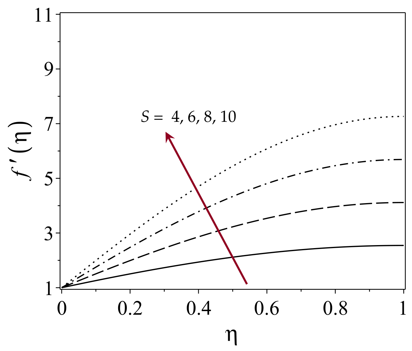
4.1. Effect of Unsteadiness on Film Thickness and Fluid Velocity

The first equation is not coupled with the second one and is the same for all cases of Table 3. It controls the dimensionless boundary layer thickness, fluid velocity and skin friction. The variable in these equations is the dimensional unsteadiness parameter S.

Table 6. Variation of velocity f${}^{\prime }$(1) and dimensionless film thickness $\beta$ with unsteadiness parameter S.

S	$\mathit{\beta }$	f${}^{\prime }\left(1\right)$	f${}^{″}\left(0\right)$
4.0	0.46222258	2.54527934	2.64859856
6.0	0.42256741	4.11506337	5.12669108
8.0	0.38196786	5.68906454	7.57845493
10.0	0.34939989	7.26442893	10.0221543

shows the effect of variation of unsteadiness S on film thickness $\lambda$, surface velocity $f^{\prime }\left(1\right)$ and skin friction $f^{″}\left(0\right)$. Figure 2 shows the variation of velocity distribution $f^{\prime }\left(\eta \right)$ in the boundary layer with unsteadiness parameter S. The film thickness $\beta$ is observed to decrease with the increase in unsteadiness S in the flow. The surface velocity f${}^{\prime }$(1) and so the skin friction f${}^{″}$(0) are observed to increase with the increase in unsteadiness S.

4.2. Effect of Unsteadiness on Temperature

As the unsteadiness in the fluid increases, the flow velocity f${}^{\prime }$($\eta$) increases. This also increases the heat flux −$\vartheta$${}^{\prime }$(0), and thus, a drop in the surface temperature $\vartheta$(1) is observed for Case 1 and Case 5. For Cases 2, 3, 6, and 7, the surface temperature $\vartheta$(1) increases with the increase in unsteadiness S in the fluid. Figure 3 and

Table 7. Variation of temperature distribution with unsteadiness parameter at Pr = 1 and $G^{*}$ = 1.

S	Case 1 and 5		Case 2, 6 and 7		Case 3
	$\mathbf{\vartheta }$$\left(\mathbf{1}\right)$	$-\mathbf{\vartheta }$${}^{\prime }\left(0\right)$	$\mathbf{\vartheta }$$\left(\mathbf{1}\right)$	$-\mathbf{\vartheta }$${}^{\prime }\left(0\right)$	$\mathbf{\vartheta }$$\left(\mathbf{1}\right)$	$-\mathbf{\vartheta }$${}^{\prime }\left(0\right)$
4.0	0.9254323	0.2063995	1.5018941	0.8804902	3.2395043	3.7582109
6.0	0.8800376	0.3375851	1.6365029	1.0733105	5.6566690	7.5566639
8.0	0.8559376	0.4088891	1.6905412	1.1414694	8.0118998	11.224076
10	0.8412676	0.4528668	1.7180535	1.1725929	10.128307	14.510949

show the effects of unsteadiness S on surface temperature $\vartheta$(1) and heat flux −$\vartheta$${}^{\prime }$(0) for all the cases.

4.3. Effect of Prandtl Number on Temperature

As the Prandtl number increases, the ratio of momentum diffusivity to thermal diffusivity increases. This increases the heat flux −$\vartheta$${}^{\prime }$(0), and thus, a temperature $\vartheta$(1) drop is observed for Case 1 and Case 5. For Cases 2, 3, 6, and 7, the surface temperature $\vartheta$(1) increases with the increase in Prandtl number Pr in the fluid. Figure 4 and

Table 8. Variation of temperature distribution $\vartheta$($\eta$) with Prandtl number at S = 4 and $G^{*}$ = 1.

Pr	Case 1 and 5		Case 2, 6 and 7		Case 3
	$\mathbf{\vartheta }$$\left(\mathbf{1}\right)$	$-\mathbf{\vartheta }$${}^{\prime }\left(0\right)$	$\mathbf{\vartheta }$$\left(\mathbf{1}\right)$	$-\mathbf{\vartheta }$${}^{\prime }\left(0\right)$	$\mathbf{\vartheta }$$\left(\mathbf{1}\right)$	$-\mathbf{\vartheta }$${}^{\prime }\left(0\right)$
0.8	0.9595775	0.1261086	1.4071290	0.7190225	2.4052188	2.3063102
1.0	0.9254323	0.2063995	1.5018941	0.8804902	3.2395043	3.7582109
1.2	0.8930815	0.2836747	1.6093876	1.0579964	4.7864442	6.2626166
1.4	0.8623943	0.3581463	1.7320289	1.2589990	7.6471113	10.783625

show the effect of Prandtl number Pr on the temperature distribution $\vartheta \left(\eta \right)$, surface temperature $\vartheta \left(1\right)$, and heat flux $-{\vartheta }^{\prime }\left(0\right)$.

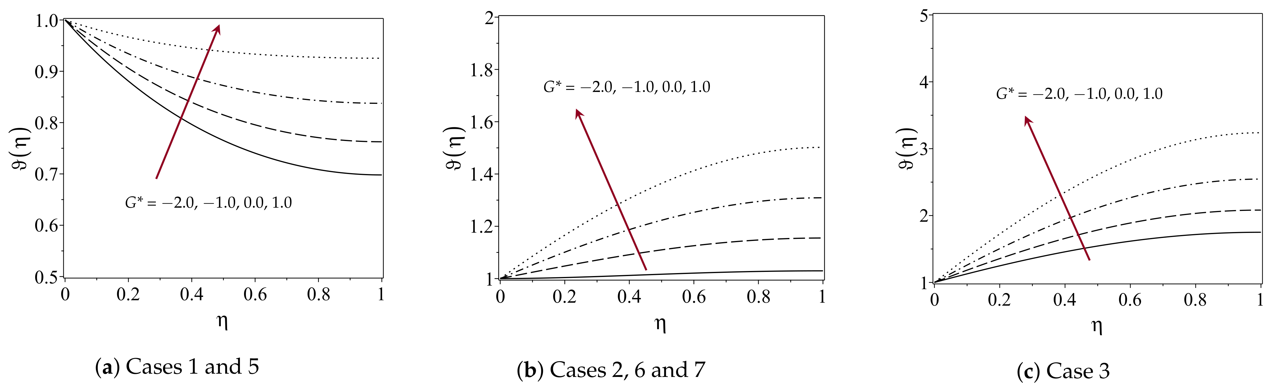
4.4. Effect of Heat Generation/Absorption on Temperature

When fluid generates heat, i.e., G${}^{*}$ > 0, the surface temperature $\vartheta$(1) increases and when it absorbs heat, i.e., G${}^{*}$ < 0, the surface temperature is $\vartheta \left(1\right)$. This corresponds to the increase and decrease in heat flux $-{\vartheta }^{\prime }\left(0\right)$, respectively. Similar effects are observed here for all cases as shown in Figure 5 and

Table 9. Variation of temperature distribution $\vartheta$($\eta$) with heat generation/absorption parameter G${}^{*}$ at S = 4 and Pr = 1.

G${}^{*}$	Case 1 and 5		Case 2, 6 and 7		Case 3
	$\mathbf{\vartheta }$$\left(\mathbf{1}\right)$	$-\mathbf{\vartheta }$${}^{\prime }\left(0\right)$	$\mathbf{\vartheta }$$\left(\mathbf{1}\right)$	$-\mathbf{\vartheta }$${}^{\prime }\left(0\right)$	$\mathbf{\vartheta }$$\left(\mathbf{1}\right)$	$-\mathbf{\vartheta }$${}^{\prime }\left(0\right)$
−2.0	0.6980416	0.6846427	1.0296499	0.0020397	1.7502717	1.3163411
−1.0	0.7626680	0.5501907	1.1551679	0.2443599	2.0816556	1.8831544
0.0	0.8376079	0.3886397	1.3090560	0.5316521	2.5452882	2.6576106
1.0	0.9254323	0.2063995	1.5018941	0.8804902	3.2395043	3.7582109

.

5. Conclusions

Reduced-order modeling has been performed by systematically deriving the similarity transformations using Lie symmetry algebra to map the system of PDEs representing heat transfer in unsteady flow with heat generation/absorption to ODEs. Similarity transformations are deduced through invariants corresponding to each linear combination of the Lie symmetries (considering two at a time) of the flow equations. These similarity transformations are used to perform double reductions to map the said system of PDEs into the system of ODES. We present only those cases here in which specific boundary conditions remain functions of both space and time variables. Seven such cases are obtained. Case 4 has not been pursued here because it has no heat generation/absorption parameter in the corresponding system of ODEs.

In all cases, the film thickness $\lambda$ = ${\beta }^2$ decreases, and the flow velocity f${}^{\prime }$($\eta$) increases with an increase in unsteadiness parameter S. For Cases 1 and 5, the surface temperature $\vartheta$(1) decreases with an increase in unsteadiness S, Prandtl number Pr and heat absorption G${}^{*}$ < 0. While for Cases 2, 3, 6 and 7, the surface temperature $\vartheta$(1) increases with increase in unsteadiness S, Prandtl number Pr and heat generation G${}^{*}$ > 0. The Lie symmetry method provides more than one type of similarity transformation and correspondingly reduces the system of ODEs, which enables a comprehensive study of the flow and heat transfer through approximate solutions of the systems of ODEs corresponding to concerned flow equations.

In this study, we show that there exists more than one type of similarity transformation which provides three different systems of ODEs when employed on PDEs describing the unsteady fluid flow and heat transfer in a boundary layer with heat generation/absorption. To the best of our knowledge, the similarity transformations and corresponding reductions of the flow model are different from those which exist in the literature. We have considered linear combinations of two symmetries by assigning a unique positive value, i.e., 1 to each coefficient in these linear combinations. Keeping arbitrary constant coefficients in these linear combinations may lead to more general forms of the similarity transformations and corresponding systems of ODEs. The inclusion of arbitrary constant coefficients in the linear combinations may yield similarity transformations and corresponding systems of ODEs with these constant coefficients. With the involvement of the arbitrary constants in resulting systems of ODEs, the convergence of the analytic solutions can be controlled, i.e., the flow and heat transfer rates can be altered with a variation in the arbitrary constants. Moreover, by constructing optimal systems of Lie sub-algebras, the classes of ODEs derived in this work can be retrieved along with maybe a few more. The inequivalence of these classes of systems of ODEs can also be established. Although the construction of optimal systems has not been included in the scope of the present study, it may lead to more general results.

References

1. Ferziger, J.H.; Peric, M.; Leonard, A. Computational Methods for Fluid Dynamics; California Institute of Technology: Pasadena, CA, USA, 1997. [Google Scholar]
2. Wang, C.Y. Liquid Film on an Unsteady Stretching Surface. Q. Appl. Math. 1990, 48, 601–610. [Google Scholar] [CrossRef] [Green Version]
3. Crane, L.J. Flow past a stretching plate. Z. Angew. Math. Und Phys. ZAMP 1970, 21, 645–647. [Google Scholar] [CrossRef]
4. Andersson, H.I.; Aarseth, J.B.; Dandapat, B.S. Heat transfer in a liquid film on an unsteady stretching surface. Int. J. Heat Mass Transf. 2000, 43, 69–74. [Google Scholar] [CrossRef]
5. Chen, C.H. Heat transfer in a power-law fluid film over a unsteady stretching sheet. Heat Mass Transf. 2003, 39, 791–796. [Google Scholar] [CrossRef]
6. Dandapat, B.S.; Santra, B.; Andersson, H.I. Thermocapillarity in a liquid film on an unsteady stretching surface. Int. J. Heat Mass Transf. 2003, 46, 3009–3015. [Google Scholar] [CrossRef]
7. Chen, C.H. Effect of viscous dissipation on heat transfer in a non-Newtonian liquid film over an unsteady stretching sheet. J. Non-Newton. Fluid Mech. 2006, 135, 128–135. [Google Scholar] [CrossRef]
8. Dandapat, B.S.; Santra, B.; Vajravelu, K. The effects of variable fluid properties and thermocapillarity on the flow of a thin film on an unsteady stretching sheet. Int. J. Heat Mass Transf. 2007, 50, 991–996. [Google Scholar] [CrossRef]
9. Liu, I.C.; Andersson, H.I. Heat transfer in a liquid film on an unsteady stretching sheet. Int. J. Therm. Sci. 2008, 47, 766–772. [Google Scholar] [CrossRef]
10. Abel, M.S.; Tawade, J.; Nandeppanavar, M.M. Effect of non-uniform heat source on MHD heat transfer in a liquid film over an unsteady stretching sheet. Int. J. Non-Linear Mech. 2009, 44, 990–998. [Google Scholar] [CrossRef]
11. Noor, N.F.M.; Hashim, I. Thermocapillarity and magnetic field effects in a thin liquid film on an unsteady stretching surface. Int. J. Heat Mass Transf. 2010, 53, 2044–2051. [Google Scholar] [CrossRef]
12. Aziz, R.C.; Hashim, I. Liquid film on unsteady stretching sheet with general surface temperature and viscous dissipation. Chin. Phys. Lett. 2010, 27, 110202. [Google Scholar] [CrossRef]
13. Aziz, R.C.; Hashim, I.; Abbasbandy, S. Effects of thermocapillarity and thermal radiation on flow and heat transfer in a thin liquid film on an unsteady stretching sheet. Math. Probl. Eng. 2012, 2012, 127320. [Google Scholar] [CrossRef] [Green Version]
14. Liu, I.C.; Megahed, A.M. Numerical study for the flow and heat transfer in a thin liquid film over an unsteady stretching sheet with variable fluid properties in the presence of thermal radiation. J. Mech. 2012, 28, 291–297. [Google Scholar] [CrossRef]
15. Aziz, R.C.; Hashim, I.; Abbasbandy, S. Flow and heat transfer in a nanofluid thin film over an unsteady stretching sheet. Sains Malays. 2018, 47, 1599–1605. [Google Scholar] [CrossRef]
16. Ibragimov, N.H. Elementary Lie Group Analysis and Ordinary Differential Equations; Wiley: New York, NY, USA, 1999. [Google Scholar]
17. Hydon, P.E. Symmetry Methods for Differential Equations: A Beginner’s Guide; Cambridge University Press: Cambridge, UK, 2000. [Google Scholar]
18. Olver, P.J. Applications of Lie Groups to Differential Equations; Springer: New York, NY, USA, 2000. [Google Scholar]
19. Szatmari, S.; Bihlo, A. Symmetry analysis of a system of modified shallow-water equations. Commun. Nonlinear Sci. Numer. Simul. 2014, 19, 530–537. [Google Scholar] [CrossRef] [Green Version]
20. Chesnokov, A.A. Symmetries of shallow water equations on a rotating plane. J. Appl. Ind. Math. 2010, 4, 24–34. [Google Scholar] [CrossRef]
21. Rashidi, M.M.; Momoniat, E.; Ferdows, M.; Basiriparsa, A. Lie group solution for free convective flow of a nanofluid past a chemically reacting horizontal plate in a porous media. Math. Probl. Eng. 2014, 2014, 239082. [Google Scholar] [CrossRef] [Green Version]
22. Siriwat, P.; Kaewmanee, C.; Meleshko, S.V. Symmetries of the hyperbolic shallow water equations and the Green Naghdi model in Lagrangian coordinates. Int. J. Non-Linear Mech. 2016, 86, 185–195. [Google Scholar] [CrossRef]
23. Xin, X.; Zhang, L.; Xia, Y.; Liu, H. Nonlocal symmetries and exact solutions of the (2+1)-dimensional generalized variable coefficient shallow water wave equation. Appl. Math. Lett. 2019, 94, 112–119. [Google Scholar] [CrossRef] [Green Version]
24. Paliathanasis, A. Lie symmetries and similarity solutions for rotating shallow water. Z. Naturforschung-Sect. A J. Phys. Sci. 2019, 74, 869–877. [Google Scholar] [CrossRef]
25. Meleshko, S.V. Complete group classification of the two-Dimensional shallow water equations with constant coriolis parameter in Lagrangian coordinates. Commun. Nonlinear Sci. Numer. Simul. 2020, 89, 105293. [Google Scholar] [CrossRef]
26. Paliathanasis, A. Shallow-water equations with complete Coriolis force: Group properties and similarity solutions. Math. Methods Appl. Sci. 2021, 44, 6037–6047. [Google Scholar] [CrossRef]
27. Abd-El-malek, M.B.; Badran, N.A.; Amin, A.M.; Hanafy, A.M. Lie symmetry group for unsteady free convection boundary-layer flow over a vertical surface. Symmetry 2021, 13, 175. [Google Scholar] [CrossRef]
28. Paliathanasis, A. Lie symmetries and similarity solutions for a family of 1+1 fifth-order partial differential equations. Quaest. Math. 2021, 45, 1099–1114. [Google Scholar] [CrossRef]
29. Safdar, M.; Ijaz Khan, M.; Taj, S.; Malik, M.Y.; Shi, Q.H. Construction of similarity transformations and analytic solutions for a liquid film on an unsteady stretching sheet using lie point symmetries. Chaos Solitons Fractals 2021, 150, 111115–111121. [Google Scholar] [CrossRef]
30. Aziz, R.C.; Hashim, I.; Alomari, A.K. Thin film flow and heat transfer on an unsteady stretching sheet with internal heating. Meccanica 2011, 46, 349–357. [Google Scholar] [CrossRef]
31. John, H.; Mathews, K.D.F. Numerical Methods Using MATLAB; Pearson Prentice Hall: Hoboken, NJ, USA, 2004. [Google Scholar]
32. Wang, C. Analytic solutions for a liquid film on an unsteady stretching surface. Heat Mass Transf.- Und Stoffuebertragung 2006, 42, 759–766. [Google Scholar] [CrossRef]
Figure 1. Schematic of flow in boundary layer.
Mathematics 10 04640 g001
Figure 2. Velocity distribution f ( η ) variation with unsteadiness parameter S.
Mathematics 10 04640 g002
Figure 3. Variation of temperature distribution ϑ ( η ) with the unsteadiness parameter S at Pr = 1 and G * = 1.
Mathematics 10 04640 g003
Figure 4. Variation of temperature distribution ϑ ( η ) with Prandtl number Pr at S = 4 and G * = 1.
Mathematics 10 04640 g004
Figure 5. Variation of temperature distribution ϑ ( η ) with heat generation/absorption parameter G * at S = 4 and Pr = 1.
Mathematics 10 04640 g005