
Statistical Descriptions of Inhomogeneous Anisotropic Turbulence

Romico Hold A.V.V., 6226 GV Maastricht, The Netherlands
Mathematics 2022, 10(23), 4619; https://doi.org/10.3390/math10234619
Submission received: 17 October 2022
/
Revised: 24 November 2022
/
Accepted: 30 November 2022
/
Published: 6 December 2022
(This article belongs to the Special Issue Analysis and Applications of Mathematical Fluid Dynamics)
Abstract
:Descriptions are given of the Langevin and diffusion equation of passively marked fluid particles in turbulent flow with spatially varying and anisotropic statistical properties. The descriptions consist of the first two terms of an expansion in powers of , where is an autonomous Lagrangian-based Kolmogorov constant: . Solutions involve the application of methods of stochastic analysis while complying with the basic laws of physics. The Lagrangian-based descriptions are converted into Eulerian-based fixed-point expressions through asymptotic matching. This leads to novel descriptions for the mean values of the fluctuating convective terms of the conservation laws of continua. They can be directly implemented in CFD codes for calculating fluid flows in engineering and environmental analysis. The solutions are verified in detail through comparison with direct numerical simulations of turbulent channel flows at large Reynolds numbers.
MSC:
37M101. Introduction
Fluid flow that exhibits turbulence is more of a rule than an exception. It occurs when the Reynolds number of the flow is sufficiently large. The number is specified as
where U [m/s] is the fluid velocity, [m2/s] is the kinematic viscosity of the fluid and L [m] is the spatial dimension of the flow configuration, e.g., the diameter of a tube, length of an air foil, or height above the earth’s surface. Values for in the cases of water and air are typically 10 and 10 m2/s, with the corresponding velocities 0.1 and 1 m/s. A configuration where m results in a value of of . This exceeds, by far, the critical value of approximately , where turbulence starts to occur.
Turbulence can be considered as a statistical process. General descriptions of the statistical parameters have yet to be found. What is known are partial results, such as the solutions for the log layer by Von Karman and the theory of the small viscous scales by Kolmogorov: e.g., Monin and Yaglom [1]. However, a general description for the statistical parameters of the large scale is missing. The key problem is the description of the statistics of the fluctuations of the convective accelerations in the governing conservation equations.
The averaged representations of the conservation equations lack well-founded statistical descriptions of the non-linear convective terms. Instead, semi-empirical versions are used, which are adapted and calibrated from case to case. These are a common feature of the methods used in fluid mechanics, including computational fluid mechanics (CFD), which are widely used in engineering and environmental analysis (Bernard and Wallace [2], Hanjalic and Launder [3]). The presented analysis does not resort to empirical construction. Instead, statistical descriptions are derived by applying the methods of stochastic analysis (Stratonovich [4], Van Kampen [5]) and obeying the basic laws of physics.
The first part of the analysis is a presentation and update of previous work [6,7,8,9] concerning the Langevin and diffusion equations for the motion of passively marked fluid particles. In the Langevin equation, the autonomous universal Lagrangian-based Kolmogorov constant appears. Its reciprocal value is about 0.14. Its smallness forms the basis for approximation. Solutions are given in descending powers of where the leading and next to leading terms are retained.
All these solutions comply with the known laws of physics. The Lagrangian-based descriptions are subsequently converted into Eulerian-based fixed-point expressions by matching using as the small parameter. They can directly be employed in the averaged equations of fluid mechanics. The outcome of the expansion is tested through comparison with the results of Hoyas et al. [10,11] and Kuerten et al. [12] for direct numerical simulations (DNS) of turbulent channel flow at a high Reynolds number.
2. Langevin Equation including Kolmogorov Similarity
Turbulent flow occurs for large values of Reynolds numbers, , a situation that is frequently encountered in practice. For , the time over which fluid particle accelerations decorrelate compares to the decorrelation times of particle velocity as to 1, e.g., [1]. This forms the basis for assuming that the velocity process can be represented by a Markov process, where accelerations are modelled as delta correlated. The corresponding Langevin equation reads as
where the time-dependent position of the moving fluid particle is described by
and . In the above equations:
Fluid velocities at a fixed point in a fixed frame of reference using the Eulerian description are indicated by , while velocities of fluid particles that move with the flow using the Lagrangian description, are indicated by . The coordinate x is used to denote a fixed position in the non-moving fixed coordinate system, while is the position of a moving particle. The turbulent flow field is considered to be stationary in a fixed frame of reference. Statistical averages of Eulerian flow variables can be calculated by time averaging, which is indicated by angled brackets or superscript . The white-noise amplitude can be specified by implementing the Lagrangian version of Kolmogorov’s similarity theory of 1941, also referred to as K-41 theory: [13] and [1] Section 21.3. This yields
where is a universal Lagrangian-based Kolmogorov constant, and is the mean energy dissipation rate averaged at a fixed position and evaluated at particle position when applied in Equation (4):
where is a fluctuating component of Eulerian velocity at fixed position .
The observation that second-order correlations of fluid particle accelerations tend to those of a delta-correlated process, when , is, in itself, not sufficient to justify the Langevin model [9]. The description of the forcing term by Gaussian white noise leads to applying ordinary non-intermittent Kolmogorov (K-41) theory. The effects of intermittency, apparent in corrections in higher-order structural functions, are not accounted for in the Langevin model [9]. For that purpose, one can adopt a fractal model based on Kolmogorov’s refined similarity theory: [1] Section 25.2.
However, the statistical averages of particle displacement that determine turbulent dispersion change little under such an approach: [1] and Borgas [14]. The effect of intermittency is apparent in small viscous scales, which govern the acceleration process, rather than in large energetic scales, which govern the velocity process of turbulence. In many applications, a Langevin model resting on K-41 theory can be considered to be a sound approach for describing the mean dispersion on distances of large-scale turbulence.
Individual values of displacement and velocity obtained from Equations (2) and (3) do not represent the actual values of fluctuating displacements and velocities of fluid particles as they occur in turbulent flow. Instead, they are dummy variables that enable the specification of statistical averages of actual fluid flow. This is achieved by generating many realizations using as a random generator and averaging the results. In the case of passive marking of fluid particles all starting at position at , the fluctuating velocities should, for every realization, be selected randomly in accordance with the distribution of the Eulerian fluctuating velocity at position :
During a simulation, the coefficients in Equations (2) and (3) vary in magnitude with the particle position in accordance with their value at . A probabilistic description of particle displacement and its velocity is obtained after performing many simulations and averaging the result at every moment in time. This enables evaluating the average spatial distribution of particles with time. This type of Lagrangian averaging is denoted by an overbar: In the case of the simulated variable , it can be written as
where is the value of f at time t in the case of simulation n.
As alternative to time simulation using the Langevin equation the same statistical distributions of fluid particle velocity and position can be obtained from the Fokker–Planck equation associated with Equations (2) and (3). It is given by
where is the joint probability density function of velocity and position at time t.
3. Specification of Damping Function by -Expansion
Thus far, I have not specified the damping term in the Langevin equation. The specification of the damping term in a form that is generally applicable has long been an issue [6,7,8,9,15]. A method was proposed in which Kolmogorov constant is used as the basis for an expansion. Solutions are described in terms of an expansion [7,8,9] in consecutive powers of . The expansion is not related to a dimensionless combination of parameters, which can attain a vanishingly small or large value. Such a combination does not exist. Instead, is used as a scaling parameter, facilitated by its autonomous position in statistical turbulence at a large Reynolds number [9].
The scaling parameter enters by the white-noise term and results in specific powers of in each of the terms on the basis of the required balances between them. The accuracy of the expansion depends on the truncation of subsequent terms. According to the measurements and data from numerical simulations, has a value of about 7: Sawford [16] and Section 9. The accuracy of the resulting expressions is discussed in Section 8 and Section 9.
Realistic solutions in the limit of are obtained from the Langevin equation when all terms scale in the same manner with . For this to happen, the damping term must scale as , and the time of correlation, which is the statistically relevant time as ; thereby, noting that the white noise term scales as . The displacement due to fluctuations during correlation scales is . This initial scaling allows for a number of approximations [9]. To the leading order in , the displacement of a particle is small, and values of fixed-point statistical quantities used in the parameters of the Langevin equation can be represented by their values at the marking point .
We can thus discuss a homogeneous statistical process in the initial stages after marking [6,7,8,9]. During that short time, the dissipation of energy by viscous action is small. The change in the Hamiltonian by viscous dissipation is small and proportional to . The statistical process is initially one that can be described by Einstein’s fluctuation theory, e.g., Reichl [17]. In the leading order formulation in powers of , the damping term is linear in velocity, satisfies Onsager symmetry, and its magnitude is determined by the fluctuation–dissipation theorem [8,9]. As a result,
where is the inverse of the covariance tensor of the Eulerian velocity field
4. Higher-Order Formulation of the Langevin Equation
Until now, attention has been focused on the leading-order term in the expansion with respect to . The resulting descriptions involve a truncation error of . Such an error will become smaller, the larger is. However, in turbulence, the value of is limited to about 7. This corresponds to and implies that the truncation error can become large. Deriving expressions for higher-order terms is, thus, desired [7]. For that purpose, one can resort to the well-mixed principle of Thomson [15]. Given an initial distribution, particles will, in the course of time, mix up with the fluid and attain the distribution of fluid velocity. This equilibrium distribution satisfies the Eulerian interpretation of Equation (8), which is given by [7]
where and is the distribution of the fluctuating component of the fixed-point Eulerian fluid velocity . There is no time derivative in Equation (11) when considering stationary turbulence: Statistical averages at a fixed point do not vary with time. Note further that is not a statistical variable but a fixed position. Statistical averages can be obtained from time averaging at fixed point . Derivatives of with respect to attain values whenever the statistical parameters of (covariances, etc.) vary in space (inhomogeneous turbulence).
The Eulerian distribution is equivalent to the non-equilibrium steady state distribution in statistical mechanics. Equation (11) represents the general form of the fluctuation–dissipation theorem that is appropriate for turbulence. Given , Equation (11) can be used to derive expressions for the damping function . Noting the leading-order formulation with respect to , cf. Equation (9), we have
where is to be determined. The Eulerian velocity distribution can be taken as Gaussian to the leading order,
where is the zero-mean Gaussian while is the correction on the Gaussian behavior. Values of the zero, first-, and second-order moments are fully captured by the Gaussian part of the description,
values of cumulants higher than second order are determined by . Substituting the description for and Equation (12) into Equation (11), one obtains, for , the equation
where there are dropped terms of relative magnitude in the contributions due to non-Gaussianity, i.e., the second term on the right-hand side of Equation (15). Equation (15) is exact, i.e., it does not involve any approximation or truncation with regard to in the case of Gaussian Eulerian velocities . The solution of Equation (15) is [7]
where ,
where is the solution of the homogeneous problem
A variety of solutions exists for , linear and nonlinear in ; however, each of them contains a degree of indeterminacy apparent in unspecified constants. When confining the damping function to linear representations in , the solution of Equation (18) is
where is the alternating unit tensor. Solution (19) constitutes an antisymmetric extension to the symmetric damping tensor derived in the previous section as described by the first term of solution (12). In this solution are three dimensionless constants whose values are unknown. It is a reflection of the nonuniqueness problem: Except for isotropic turbulence, it is impossible to fully specify the damping function on the basis of a specified fixed-point Eulerian velocity distribution. Yet, there is a practical way out of the nonuniqueness problem [7,8,9].
It appears that yields only contributions of relative magnitude compared to the previously determined leading terms in the statistical distributions of particle displacement. This conclusion is arrived at when deriving the diffusion equation from the Langevin equation: see Section 5. This reveals the contributions of relative magnitude in diffusivity and convection only. The same result is obtained for the other term in solution (17), which describes the effect of non-Gaussianity. In general, the contribution of in solution (16) can be disregarded in any description, which allows for a relative error of in the diffusion limit. Setting , we arrive at a Langevin model, which has, as a damping function,
While the first term in this solution corresponds to the result of the Hamiltonian base case, the second and third terms represent the correction due to inhomogeneity in an otherwise locally homogeneous statistical field. The corrections can be related to the change of energy, which was disregarded in the leading-order formulation where underlying particle mechanics can be considered Hamiltonian [7,8]. The second term describes the change of energy due to changes of covariances in the direction of the mean flow. Accelerating or decaying the mean flow results in non-zero values of the second term. The third term describes the effects of the spatial gradient of the fluid velocity covariance. This can be associated with shearing due to external forcing.
Solution (20) corresponds to a previous result of Thomson [15]. It was one of several proposals made for the damping functions, which all satisfy the well-mixed criterion and which correspond to an entirely Gaussian Eulerian velocity distribution. This is a reflection of indeterminacy because of the nonuniqueness. The present analysis provides an answer. It reveals descriptions for statistical displacement obtained from Equation (20), which are unique up to an error of .
5. The Diffusion Limit
The diffusion limit concerns the description of random particle displacements on a time scale that is much larger than the correlation time of the fluctuating velocity. As indicated by a balance between the acceleration term and damping term in the Langevin equation, the correlation time can be expressed as
where is the magnitude of velocity flucutations and is the characteristic time of large scales or of the eddy turn-over time. The description of the time scale is known as coarse graining, e.g., [1] vol.I, Section 10.3. The magnitude of the fluctuating fluid particle displacement during correlation can be represented by
where represents the size of the eddies, which is also the distance over which the statistical parameters vary in magnitude.
The Langevin model is centered around the fluctuating particle velocity relative to the mean Eulerian velocity: cf. Equations (2) and (3). In line with this representation, the displacement of a fluid particle by the sum of a component due to the mean flow and a component representing the zero-mean random displacement are described (see also [18] and [5] Section XVI.5):
where is the particle track according to the Eulerian mean velocity:
For general inhomogeneous turbulent flow, the Eulerian-based coefficients in the Langevin model vary in magnitude with the space coordinates. This makes the coefficients time-dependent in the Langrangian-based description of the Langevin model. Representing displacement by Equation (23), the time dependency occurs in two ways [8]: (i) through spatial variations when following the particle according to the mean velocity and (ii) through dependency on random displacement
In the next analysis, I shall disregard the dependency on . Furthermore, I disregard the non-linear third term in the damping function as well as . Requiring the Gaussian behavior in the leading order formulation and mixing for next-to-leading order, all these terms yield contributions of relative magnitude in the diffusion model: see Appendix of [8]. The Langevin model, which specifies diffusion to the leading order and next-to-leading order now follows from Equations (2) and (3) as
From Equations (3), (23) and (24), we obtain
Fluctuating Equations (26) and (27) can be transformed into a Fokker–Planck equation for the joint probability of and . The solution is a multi-dimensional Gaussian distribution with time-dependent parameters: [5] Section VIII.6. The zero-mean probability density distribution for the fluid particle position in the fixed coordinate system , which moves with the mean Eulerian velocity is specified by the diffusion equation
subject to a suitably chosen initial distribution at , i.e., the delta pulse in the case of passive marking of particles at and . Note that the time derivative in the above Eulerian description applies to the coordinate system, which moves with the mean velocity according to Equations (23) and (24) . To evaluate the diffusion coefficient , note that
where the latter term can be calculated by multiplying Equation (26) with and averaging
There is no contribution of the last term of Langevin Equation (26) because is only correlated with . Substituting Equation (30) into the r.h.s. of Equation (29) results in the following first-order differential equation for the diffusion coefficient
subject to the initial condition at . The equation describes the transient of the diffusion coefficient towards its value valid in the diffusion limit when . This limit value can be time-dependent on the time-scale and can be obtained by iteration using as the small parameter [8]. The leading order follows from a balance between the second term on the l.h.s. and the first term on the r.h.s. Substituting this solution into the neglected other terms and noting that, according to our definitions, when , we obtain, in terms of the Eulerian coordinates of the non-moving frame [8]
The leading order term in the diffusion tensor is symmetric; however, the terms that are next to the leading order are not. However, the non-symmetric part of the tensor is found to make contributions of in the convection of fluid particles and admixture only: [8]. The non-symmetric part makes no contribution to the next-to-leading order terms in the diffusion coefficient.
In the above derivation, I considered the limit by which velocities de-correlated from their initial value at . At the same time, one can take , which is the time scale of the large eddies and the time scale of inhomogeneous behavior. Under this condition, the values of parameters can be represented by their values at the initial marking: . As one can repeat the derivation for any other point of marking, one can replace by : i.e., and in (32).
The diffusion equation in a non-moving Eulerian frame now follows from Equations (28) and (32) as
where is the probability density of a marked fluid particle at position and time t. The probability distribution applies equally to parameters whose values are linearly connected to the value of the particle position: i.e., concentrations of passive or almost passive admixtures, such as aerosols or the temperature in incompressible or almost incompressible fluids; see also Section 7. To determine the distributions from (33), the mean values , co-variances and mean dissipation rates need to be known. These can be obtained using techniques of Computational Fluid Dynamics.
6. Statistical Descriptions of Momentum Flux
Momentum flux plays a central role in the conservation equations of fluid mechanics. An issue is the specification of the Reynolds stresses, i.e., the mean value of the fluctuating components of the momentum flux tensor. The conservation equations are typically formulated with respect to a fixed coordinate system, viz. the Eulerian formulation. The aim of the present analysis is to derive expressions for the mean value of the fluctuating components that fit in the Eulerian frame. First, the Lagrangian-based momentum flux tensor is considered where are the velocities of moving fluid particles that all pass at through the surface at (alternatively, one can choose the velocity and the surface but with ultimately the same Eulerian result due to the symmetry of the diffusion tensor).
Statistical averages are determined at close distance from using Lagrangian-based expressions for , which were derived in the previous sections. Taking the diffusion limit of the Lagrangian-based solutions and letting the distance from approach zero on the coarse scale of the diffusion approximation, a connection can be made with the Eulerian-based value of the tensor: . This enables the completion of the description of the averaged representation of the conservation equations of momentum for fluid mechanics.
The displacement of a marked fluid particle that is at position at time follows from (3) as
where is value of the Eulerian mean velocity at particle position and
To describe the position of the particle at times close to , expand the r.h.s. of (35) as:
where is the Eulerian mean velocity at . Neglected terms on the r.h.s. of (36) are larger than the quadratic in t and . It can be shown that these terms only contribute to in the diffusion approximation. In accordance with the above expansion, the particle velocity is described by
The objective is to describe the average momentum of particles that approach the surface at with velocity . The particles are situated in an area that is small compared to the size of the large eddies so that Eulerian statistical averages can be treated as homogeneous in space. Furthermore, the area considered is large compared to the area where the particle velocities are correlated. For these conditions to be satisfied, , which is the condition for the diffusion limit to apply. This involves a limit process whereby time approaches zero but on the time scale of coarse graining of the diffusion limit: , where is the correlation time of the particle velocities.
The momentum for small negative times is given by
The average value of the momentum of all particles passing the surface is
with the property that and at . Fluid particles will cross the plane at different positions. However, the particles under consideration are in an area whose size is limited. The spatial variations of the mean Eulerian velocities are small and can be disregarded within the order of approximation of the developed perturbation scheme. In (39), they are taken to be equal to the value at the point of the crossing of (38).
When applying Langevin Equation (2) to negative values of t, the damping term has to change sign in order to yield the required decay with . Hence, , , and
The correlation can be determined in accordance with (31) and (32), where the energy dissipation rate and the co-variances can be taken to be equal to their values at under the limit process of the diffusion limit. The result equals the expression for the diffusion coefficient of (32).
When shear and mean flow gradients are absent, an isotropic state exists, a feature that is seen in grid turbulence. In this case,
where is the kinetic energy of the isotropic state. Invoking (40)–(42) in (39), we have
Result (43) applies in an area where the diffusion limit holds. The area is of volume where and where is the length of velocity correlations and L is the size of the large eddies or flow configuration. The presented descriptions are valid in the limit of , . The smallness of is limited: . Yet, comparison with a range of results of measurements and direct numerical simulations shows fairly good agreement (Section 9). The reason is that terms of order are incorporated into the expansion, and the correlations decay exponentially with time where is the eddy turnover time (cf. Equation (21)).
Reducing the volume of the area to zero, it becomes identical to a point in the Eulerian description of the flow field. We can, thus, take
The mean value of the fluctuating kinetic energy k is given by
where repeated indices n imply summation. Substituting (47) into (48), one obtains
which can be used to eliminate from (47) with the result
Similar to the analysis in the previous section, one can repeat the above procedures for any other point and extend the results (45) and (50) to all positions by replacing by . The resulting statistical descriptions account for inhomogeneity of the turbulence field.
Equation (50) allows all six co-variances to be determined for given values of k, , and . Having implemented Equations (32), (45), (46) and (50), the values of the mean velocities can be derived from the averaged versions of the equations of conservation of momentum. To obtain a closed set of equations, two equations determining k and have to be included. In this respect, it is noted that relation (48) is implied by (50) and does not represent an extra relation for k. The extra equations are provided by the two equations of the model that describes these variables [2,3]. The closed system of coupled equations, thus, obtained is a straightforward extension of the equations of the widely used model. The model may be termed the anisotropic model, and this enables the mean values of the statistical parameters of an anisotropic inhomogeneous turbulent flow to be calculated.
7. Statistical Descriptions of Scalar Flux
Examples of scalar flux are the dispersion of substances immersed in fluids and of temperature distributions in incompressible and almost incompressible fluids. Turbulence is known to have a significant effect on these phenomena. Similar to the analysis of the previous section, consider an area that is small to the area of inhomogeneity but large compared to the area where particle velocities are correlated. The Lagrangian scalar flux is described by , where are the velocities of marked fluid particles that all pass at through a surface at , and is the value of the scalar quantity at the position of each moving particle. When considering the velocities of particles at a short distance, the time from the surface of passing (37) can be employed. For the value of the scalar quantity at the position of the particle, we have
The first and second term on the right-hand side represent dispersion of the scalar quantity due to fluid particle displacement whereby the scalar does not vary in magnitude while moving with the fluid particle. The third term is autonomous random changes of the value of the scalar quantity while moving with the fluid particle. For the first term, take the Eulerian-based mean value at . Similar to the analysis of the previous section, particles pass through different positions at the surface . However, all these positions are at a limited distance from each other in accordance with the coarse graining of the diffusion limit.
On this scale, spatial variations in value of the first term of the expansion can be disregarded. They can be taken to be equal to the Eulerian mean value at the single point . Furthermore, the first term is allowed to vary deterministically with time , where is the time in the Eulerian fixed frame of reference: . Lagrangian averaging can take place by adding the simulation results of the Langevin equations at a fixed value of and subsequently repeating for every other value of . The variation with is considered to be slow compared to the rapid variation of the random fluctuations of .
Multiplying the right-hand sides of Equations (37) and (51), replacing t by , applying Lagrangian averaging and letting after applying the diffusion limit, one obtains (similar to the procedure of the previous section)
The third and fourth terms on the right-hand side are contributions due to autonomous fluctuation of the scalar when moving with the fluid particles. To determine the values of these terms, fluctuation equations of need to be known. No attempts will be made to derive such equations. We assume that is a conserved quantity whose value does not change while moving with the fluid particle: . Noting that
and implementing (41) then yields
where equals the Eulerian-based value at . As the relation holds for every position x, we have
where is a conserved quantity that satisfies the Eulerian-based conservation equation
Applying equation ensemble averaging to the above, substituting Equation (55) and replacing by t, yields
where I employed the averaged version of continuity: . The above result equals the equation for fluid particle distribution given by Equation (33). This is consistent with the feature that the distribution of the particle must be equal to the distribution of a conserved quantity whose value does not change with value of following the path of a fluid particle.
8. Decaying Grid Turbulence
Decaying grid turbulence has been studied many times during the previous century, and many results are available. Turbulence is generated by a uniform mean flow that passes through a grid of squarely spaced bars. The grid is perpendicular to the incoming mean flow. At some distance behind the grid, a homogeneous field of isotropic turbulence develops and decays in the downstream direction with the mean flow. For grid turbulence, exact results for the Langevin and diffusion equations are known. In the present section, I recapitulate these results and compare them with the present results based on the two-term expansion.
For convenience in presentation, turbulence is described in a frame that moves with the uniform mean velocity. I thus describe the equivalent situation where the grid moves with constant speed from right to left through a fluid that is initially at rest. When the grid has passed, a uniform field of isotropic zero-mean Gaussian fluctuations exists, which decays in time. The strength is the same in all three coordinate directions. Therefore, analysis is restricted to fluctuations in one direction only. Corresponding variables are indicated by a subscript of 1. Regarding the independence of fluctuations in three directions, a problem of nonuniqueness, as discussed in Section 5, does not exist. The appropriate Langevin equation in one-dimensional form can be written as
where is the Eulerian mean square of the fluctuations
Expressions for and can be derived from the Von Karman-Howarth equation for conservation of the mean kinetic energy of fluctuations. For large Reynolds numbers, these expressions are: [19]
where is the reference time, i.e., a moment in time where the grid has passed the observer at a fixed position. The value of depends on the dimensioning of the grid and can be established by measurements at time . Implementing (60) into (58), we have
From this result, one can derive (analogous to the derivation in Section 5) the diffusion equation
where the diffusion coefficient is given by
Note that the diffusion coefficient does not decrease in the stream-wise direction. A decay in the strength of fluctuations is compensated for by an increase in the correlation time.
Results (61)–(63) were obtained without using the expansion. The Langevin equation according to a two term expansion is given by Equations (2) and (20). Introducing the features of grid turbulence results in an equation that is the same as Equation (61). The diffusion coefficient according to the two term expansion is given by Equation (32). This reduces, in the case of grid turbulence, to . Expanding the exact result given by Equation (63) in powers of yields .
The first two terms in the diffusion coefficient of the exact result thus agree with the two-term expansion. The third term amounts to a relative contribution of 0.9% when . In conclusion, the two-term expansion complies with the corresponding expansion of the exact result, and the error of truncating the third term is small. The latter conclusion is, however, of limited value as the grid turbulence is isotropic and only slightly inhomogeneous in the stream-wise direction. In practice, turbulence is mostly anisotropic and appreciably inhomogeneous. The next section analyses such a case.
9. Turbulent Channel Flow
Turbulence is a well-known feature of flows in pipes and channels and in boundary layers along walls, including the boundary layers along the earth’s surface. A representative case for such flows is a developed turbulent flow in a channel of two parallel flat plates. The statistical values are constant in the direction of the mean flow between the plates and in the direction that is parallel to the plates and perpendicular to the mean flow but changes significantly in magnitude in the direction normal to the plates. The fluctuations are strongly anisotropic.
9.1. Exact Results
Some exact results can be derived from the averaged Navier–Stokes (N-S) Equations: ([1] vol I, p. 268). The averaged equations are given by
where p is the pressure relative to the pressure of the fluid at rest, and is the density. In the case of a developed turbulent channel flow, the mean values involving fluctuating velocities and pressure gradients vary only with the wall normal coordinate . The averaged N-S equations then reduce to
where is the coordinate of the mean flow direction, are the co-variances of fluctuating velocities, and is the mean pressure. The contribution of the viscous stress represented by the last term in Equation (64) was disregarded in the above equations. The effect is limited to thin viscous layers near the wall. Their effect on the flow outside these thin layers can be accounted for by the boundary condition imposed on the shear stress at the wall. From Equations (65) and (66), one obtains the solutions
where is the shear velocity and is the distance between the parallel plates. The shear velocity can be related to the pressure drop in the channel by solving the flow in the boundary layer at the wall. The relationship is also known from measurements: e.g., [1]. The value of is representative for the magnitude of the fluctuations.
9.2. Results from the -Expansion
The exact results of Section 9.1 can be extended by supplementing the expressions for the turbulent momentum diffusion of Equation (50). For the channel flow, these become
where is the mean flow in the channel and where the diffusion coefficients are given by
Equations (67)–(74) constitute eight relations for 10 variables: and . A closed system of equations requires two extra equations. These are provided by the conservation equations for kinetic energy k and dissipation rate known from CFD models [2,3]. Our aim is not to study a complete and closed system of equations but to analyze all those components that describe turbulent transport in such equations. For this purpose, one can calculate the values of the left-hand sides and right-hand sides of the developed relations using the data of direct numerical simulations and compare them with each other. This provides a direct test of the outcome of the expansion. An article in which the complete set of equations is formulated and analyzed is in preparation.
9.3. Comparison with the DNS Results
Super computers have created the possibility to simulate turbulent fluid flows through direct numerical simulations (DNS) of the equations that govern fluid flow, i.e., the Navier–Stokes equations. Initially, attention was focused on grid turbulence at modest values of Reynolds numbers. The calculation power has increased with time. This allows handling flows at larger Reynolds numbers and with more complex configurations of channel flow. Hoyas et al. [11] recently published results for channel flow at a friction Reynolds number of . This corresponds to a bulk flow Reynolds number of about . DNS is the most reliable technique to study turbulence, and its outcome can be considered as exact. The results of Hoyas et al. provide an excellent opportunity to verify the present results.
9.3.1. Statistical Values of Fluctuations
Making dimensionless by and k by by H and P and by , and dropping the subscript 2 from , one can derive, from Equations (67)–(74), the relations
where
and P is the production of energy defined as
From Equations (75)–(77), it can be verified that, at : . This is consistent with the solution for a zero mean flow gradient. At , the solutions for the log law apply, according to which, . From Equations (75)–(77), one then finds
These reveal anisotropy whose magnitude depends on the magnitude of .
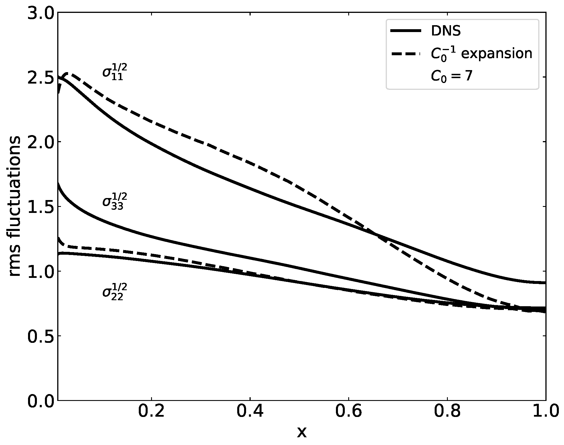
Figure 1 shows the values of the root mean square of fluctuations according to Equations (75)–(77) versus x for taken from DNS and . The values are compared with the corresponding DNS values of these parameters. Close to the wall at , the effect of the viscous layer is seen. Its thickness is about , which amounts to 1% of the height of the channel. The results of the expansion only apply outside this area. Here, it is seen that strong anisotropy in the longitudinal direction is predicted.
A difference between fluctuations in normal and the span-wise direction as forecast by DNS is not revealed. Differences between the longitudinal fluctuations and normal fluctuations near the axis are not revealed either. Near , differences between rms values in the normal and span-wise direction are at maximum. The differences between longitudinal and transverse fluctuations are at a maximum at . Otherwise, the differences between the DNS and expansion are rather limited—keeping in mind the limited smallness of the perturbation parameter .
9.3.2. Statistical Values of Turbulent Fluxes
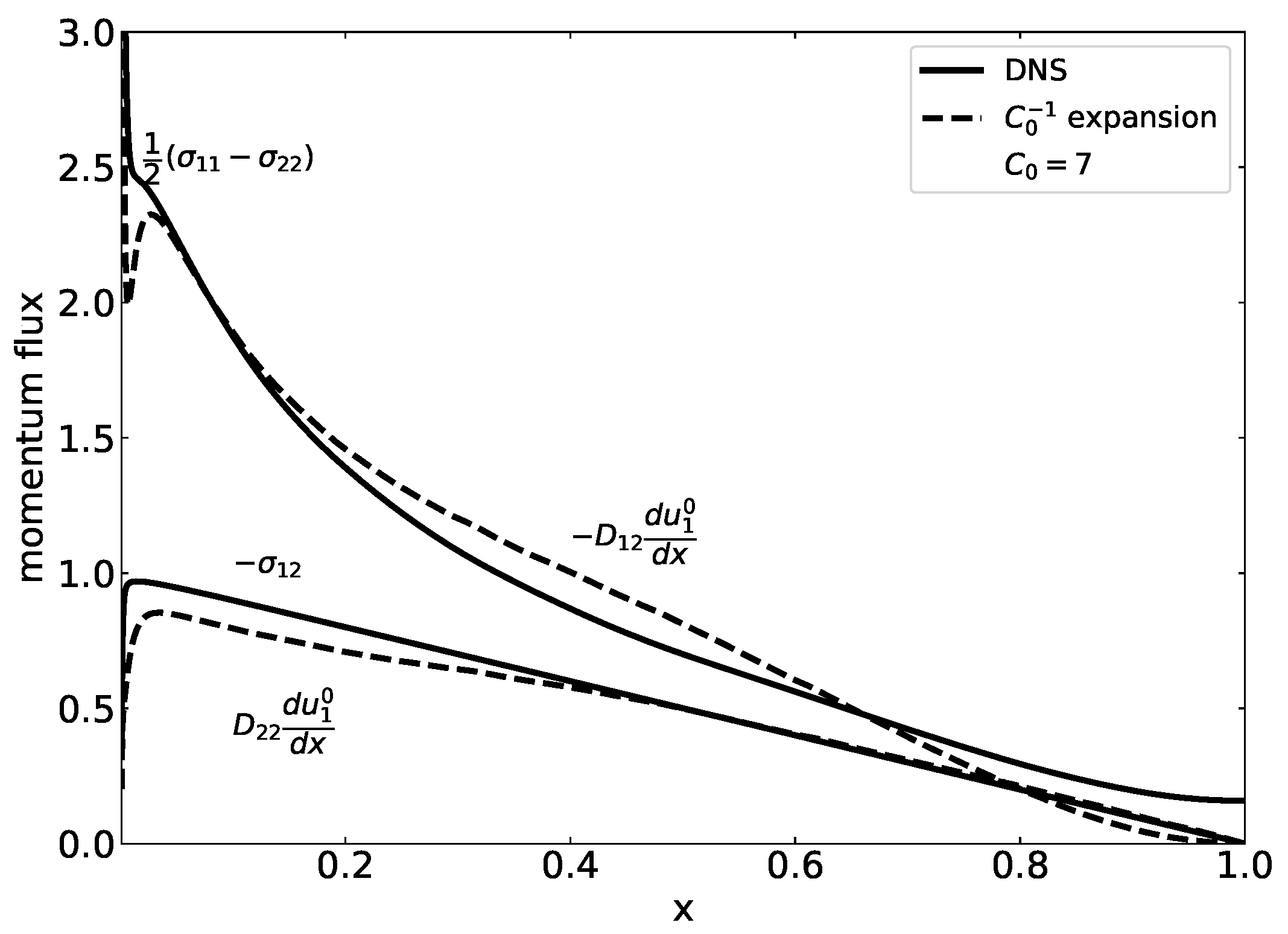
An issue in turbulence theory is the statistical description of the non-linear fluctuating convective terms in the equations of conservation of momentum and energy. The issue is known as the closure problem. The present analysis provided an answer by the expressions for turbulent flux and turbulent diffusion coefficients. Figure 2 and Figure 3 present the results obtained for these terms and compare them with the DNS results.
9.3.3. Diffusion Coefficients
9.3.4. Kolmogorov Constant
In general, it is found that a value of 7 for gives a good fit to the DNS. This value is somewhat higher than the value of 6.2 mentioned previously considering the DNS of turbulent channel flow at of [8]. A value of of 7 at high Reynolds number has been claimed by Sawford referring to DNS of grid turbulence [16].
10. Conclusions
The presented statistical descriptions fit within the asymptotic structure of turbulence at a large Reynolds number with Kolmogorov theory. The descriptions apply to large scales, which determine the main flow outside small viscous boundary layers at adjoining walls of the configuration considered. The given representations of the velocity and position of marked fluid particles are Lagrangian-based and concern Langevin and diffusion equations. In these equations, the universal Kolmogorov constant appears with a value of about 7. This is used as an autonomous parameter in developing solutions by the first two terms of perturbation expansions in powers of . The leading solution complies with the conditions of Hamiltonian dynamics, Gaussian behavior and Onsager symmetry as . The second term of the solution satisfies mixing with the Eulerian-based statistical distribution of the flow field.
The Lagrangian-based descriptions were connected to Eulerian statistics through asymptotic matching. When considering a small but sufficiently large area around a fixed point in space where the diffusion limit applies, shrinking this area to a point accomplishes matching the Eulerian description at the corresponding point. The matching involves the limit process , where is required for obtaining the diffusion limit, and to ensure that the considered area is much smaller than the area of inhomogeneous behavior of the main flow.
The two-term descriptions meet the requirements that follow from the laws of physics and the methods of stochastic analysis. The presented solutions reveal the functional relationships between the statistical averages of various fluctuating quantities, such as turbulent diffusivity. They do not rely on semi-empirical hypotheses and fitted constants. Limiting factors include inaccuracies due to truncation of the higher order terms. For slowly decaying grid turbulence, these are small. However, in the case of strong inhomogenity, the matching of Lagrangian and Eulerian results appears to require small values of , . Yet, comparison with the DNS of turbulent channel flow at high Reynolds number reveals deviations of limited magnitude despite large inhomogeneity and anisotropy.
An underlying reason is likely the inclusion of next to leading terms and exponential decay of velocity correlations by , where is the eddy turnover time or characteristic time of large-scale turbulence: (21).
The results for the main Eulerian statistical parameters in the case of channel flow are shown in Figure 1, Figure 2 and Figure 3. They reveal fairly good agreement between the predictions of the model when compared with those of DNS. This conclusion applies to turbulent channel flow, which is a case of turbulence that is significantly anisotropic and inhomogeneous. As the model has a general basis, this entails the prospect of yielding reliable results for other cases of anisotropic inhomogeneous turbulent flow.
Funding
This research received no external funding.
Informed Consent Statement
Not applicable.
Data Availability Statement
Not applicable.
Acknowledgments
Conflicts of Interest
The author declares no conflict of interest.
References
- Monin, A.S.; Yaglom, A.M. Statistical Fluid Mechanics; Dover: New York, NY, USA, 2007; Volumes 1–2. [Google Scholar]
- Bernard, P.S.; Wallace, J.K. Turbulent Flow: Analysis, Measurement and Prediction; Wiley: New Jersey, NJ, USA, 2002. [Google Scholar]
- Hanjalić, K.; Launder, B. Modelling Turbulence in Engineering and the Environment: Second-Moment Routes to Closure; Cambridge University Press: Cambridge, UK, 2011. [Google Scholar] [CrossRef]
- Stratonovich, R.L. Topics in the Theory of Random Noise; Gordon and Breach: New York, NY, USA, 1967; Volume 1. [Google Scholar]
- van Kampen, N.G. Stochastic Processes in Physics and Chemistry, 3rd ed.; Elsevier: New York, NY, USA, 2007. [Google Scholar]
- Brouwers, J.J.H. Langevin and diffusion equation of turbulent fluid flow. Phys. Fluids 2010, 22, 085102. [Google Scholar] [CrossRef] [Green Version]
- Brouwers, J.J.H. Statistical description of turbulent dispersion. Phys. Rev. E Stat. Nonlinear Soft Matter Phys. 2012, 86, 066309. [Google Scholar] [CrossRef] [PubMed] [Green Version]
- Brouwers, J.J.H. Statistical Models of Large Scale Turbulent Flow. Flow Turbul. Combust. 2016, 97, 369–399. [Google Scholar] [CrossRef] [Green Version]
- Brouwers, J.J.H. Statistical Model of Turbulent Dispersion Recapitulated. Fluids 2021, 6, 190. [Google Scholar] [CrossRef]
- Hoyas, S.; Jiménez, J. Scaling of the velocity fluctuations in turbulent channels up to Reτ = 2003. Phys. Fluids 2006, 18, 011702. [Google Scholar] [CrossRef] [Green Version]
- Hoyas, S.; Oberlack, M.; Alcántara-Ávila, F.; Kraheberger, S.V.; Laux, J. Wall turbulence at high friction Reynolds numbers. Phys. Rev. Fluids 2022, 7, 014602. [Google Scholar] [CrossRef]
- Kuerten, J.; Brouwers, J.J.H. Lagrangian statistics of turbulent channel flow at Reτ = 950 calculated with direct numerical simulation and Langevin models. Phys. Fluids 2013, 25, 105108. [Google Scholar] [CrossRef] [Green Version]
- Kolmogorov, A. The Local Structure of Turbulence in Incompressible Viscous Fluid for Very Large Reynolds’ Numbers. Akad. Nauk. Sssr Dokl. 1941, 30, 301–305. [Google Scholar]
- Borgas, M.S. The Multifractal Lagrangian Nature of Turbulence. Philos. Trans. Phys. Sci. Eng. 1993, 342, 379–411. [Google Scholar]
- Thomson, D.J. Criteria for the selection of stochastic models of particle trajectories in turbulent flows. J. Fluid Mech. 1987, 180, 529–556. [Google Scholar] [CrossRef]
- Sawford, B.L. Reynolds number effects in Lagrangian stochastic models of turbulent dispersion. Phys. Fluids A Fluid Dyn. 1991, 3, 1577–1586. [Google Scholar] [CrossRef]
- Reichl, L.E. A Modern Course in Statistical Physics; Wiley-VCH: Hoboken, NJ, USA, 2004. [Google Scholar]
- Brouwers, J.J.H. On diffusion theory in turbulence. J. Eng. Math. 2002, 44, 277–295. [Google Scholar] [CrossRef]
- George, W.K. The decay of homogeneous isotropic turbulence. Phys. Fluids A 1992, 4, 1492–1509. [Google Scholar] [CrossRef]
Figure 1.
The root mean square values of the velocity fluctuations versus the dimensionless distance from the wall. The root mean square values obtained from DNS are represented by full lines. The root mean square values of the expansion are represented by broken lines. They result from Equations (75) and (76) in which the right-hand sides were evaluated using the DNS values. Differences between full and broken lines can be ascribed to truncation of the expansion.

Figure 2.
The mean momentum fluxes versus the dimensionless distance from wall. The values of and are obtained using DNS and are represented by full lines. The values of and result from the expansion and are represented by broken lines. They follow from Equations (69), (71) and (72) in which the right-hand sides were evaluated using the DNS values.

Figure 3.
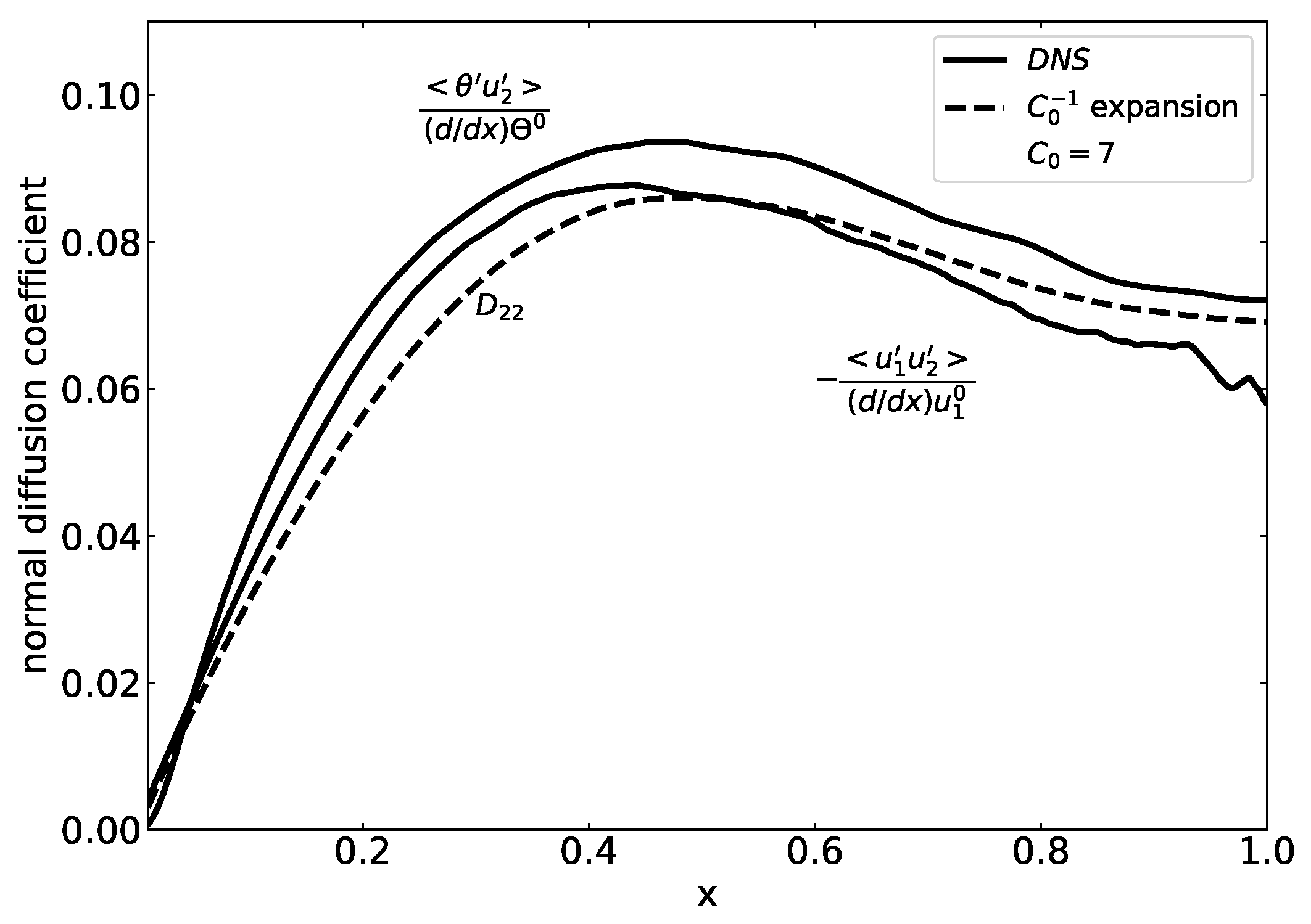
Coefficients of diffusion in the wall normal direction for momentum transport and heat transport versus dimensionless distance from wall. The values of and are obtained using DNS and are presented by full lines. The values of result from the expansion. They follow from Equation (74) in which the right-hand side was evaluated using the DNS values. They are represented by a broken line.
Figure 3.
Coefficients of diffusion in the wall normal direction for momentum transport and heat transport versus dimensionless distance from wall. The values of and are obtained using DNS and are presented by full lines. The values of result from the expansion. They follow from Equation (74) in which the right-hand side was evaluated using the DNS values. They are represented by a broken line.

Publisher’s Note: MDPI stays neutral with regard to jurisdictional claims in published maps and institutional affiliations. |
© 2022 by the author. Licensee MDPI, Basel, Switzerland. This article is an open access article distributed under the terms and conditions of the Creative Commons Attribution (CC BY) license (https://creativecommons.org/licenses/by/4.0/).
Share and Cite
MDPI and ACS Style
Brouwers, J.J.H. Statistical Descriptions of Inhomogeneous Anisotropic Turbulence. Mathematics 2022, 10, 4619. https://doi.org/10.3390/math10234619
AMA Style
Brouwers JJH. Statistical Descriptions of Inhomogeneous Anisotropic Turbulence. Mathematics. 2022; 10(23):4619. https://doi.org/10.3390/math10234619
Chicago/Turabian StyleBrouwers, J. J. H. 2022. "Statistical Descriptions of Inhomogeneous Anisotropic Turbulence" Mathematics 10, no. 23: 4619. https://doi.org/10.3390/math10234619
Note that from the first issue of 2016, this journal uses article numbers instead of page numbers. See further details here.