Convolution Based Graph Representation Learning from the Perspective of High Order Node Similarities

Abstract

Nowadays, graph representation learning methods, in particular graph neural network methods, have attracted great attention and performed well in many downstream tasks. However, most graph neural network methods have a single perspective since they start from the edges (or adjacency matrix) of graphs, ignoring the mesoscopic structure (high-order local structure). In this paper, we introduce HS-GCN (High-order Node Similarity Graph Convolutional Network), which can mine the potential structural features of graphs from different perspectives by combining multiple high-order node similarity methods. We analyze HS-GCN theoretically and show that it is a generalization of the convolution-based graph neural network methods from different normalization perspectives. A series of experiments have shown that by combining high-order node similarities, our method can capture and utilize the high-order structural information of the graph more effectively, resulting in better results.

1. Introduction

Graph is a flexible data modeling and storage structure, which is widely used in biology [1,2], sociology [3], engineering [4] and other fields. With the advent of the big data era, the graph structure becomes more and more complex. For this reason, among various technical tools for studying graphs, GNNs (graph neural networks, data-driven deep learning methods) have evolved rapidly and excelled in many important problems, such as node classification [5] and community detection [6].

One of the earliest studies on GNNs can be traced back to the work of Scarselli et al. [7], which has sparked a great deal of research interest among researchers. After that, Bruna et al. [8] first introduce convolution into GNNs. Subsequently, Defferrard et al. [9] and Kipf et al. [5] successively make optimization of the graph convolution operation and the resulting model GCN (graph convolution network) is one of the most popular basic models now. Another very famous base model is GAT (graph attention network) introduced by Velickovic et al. [10], in which the attention mechanism [11,12] is applied.

Based on the success of GCN and GAT, a large number of methods [13,14,15,16] and applications [17,18,19,20] have been developed. However, the GCN model uses only the graph adjacency matrix and can not assign different weights to each neighbor. More specifically, the GCN treats all neighbor nodes equally during convolution and can not assign different weights based on node importance. As for GAT model, it learns the weight parameters of node neighbors through the attention mechanism, which allows assigning different importance to neighboring nodes. However, this approach ignores the prior information of nodes, which is stored in the graph structure. On the other hand, most of these methods utilize only the edge structure, ignoring the important role of high-order structures in the information transfer process.

Present work. In this paper, we introduce HS-GCN, which is a graph convolutional network combining high-order node similarity features. HS-GCN can exploit node similarities to mine the potential structural features of the graph from different perspectives and assign different weights to node neighbors. We also analyze theoretically that these different perspectives are actually equivalent to different normalizations of the weight matrix. At the same time, we have conducted a large number of experiments. The experimental results and analyses have shown that by combining node similarities, our method can capture and utilize the structural information of the graph more effectively, resulting in better results. In particular, the results are even better when combining high-order node similarities, since the structural information is richer.

In fact, it is worth noting that our method is a framework that can combine arbitrary node similarities. Because we believe that high-order node similarities contain richer structural information (it is confirmed in our experiments), three representative high-order similarities are selected as specific implementations.

The rest of this paper is organized as follows. In Section 2, we present related work including the general architecture of GNNs and several node similarities utilized in this paper. Then our method is described in detail in Section 3. The experiments are arranged in Section 4. Finally, the conclusion part is in Section 5.

2. Related Work

In this part, we focus on previous work closely related to our method. First, some notations are agreed: let $G=(V,E)$ denote a graph, where V is the node set ($v\in V$) and $E\subseteq (V\times V)$ denotes the set of edges. If node u and node v are connected in graph G, then $(u,v)\in E$. $A\in {\{0,1\}}^{n\times n}$ is the adjacency matrix of G, where $n=\left|V\right|$ is the number of nodes and if $(v_i,v_j)\in E$, then $A_{i,j}$ (the element on row i and column j of A) is 1, the others are 0:

$$\begin{array}{c}\hfill A_{i,j}=\left\{\begin{array}{cc}1,\hfill & \mathrm{if}({\mathrm{v}}_{\mathrm{i}},{\mathrm{v}}_{\mathrm{j}})\in \mathrm{E};\hfill \\ 0,\hfill & \mathrm{otherwise}.\hfill \end{array}\right.\end{array}$$

(1)

2.1. Graph Neural Networks

GNNs generalize deep learning methods to graph structured data [21,22] and have recently produced many successful applications in many areas, such as recommendation system [23], transportation [24], image processing [25], etc. In general, GNNs follow a two-stage operation of “aggregation” and “update”. Specifically, GNNs get “message” from neighbor nodes in the first stage; and then GNNs update the representation of the central node. The form can be expressed as follows:

$$h_{N_{\left(v\right)}}^{(k+1)}={\mathrm{M}}^{\left(k\right)}(\{h_u^{\left(k\right)},h_v^{\left(k\right)}|u\in N_{\left(v\right)}\}),$$

(2)

$$h_v^{(k+1)}={\mathrm{U}}^{\left(k\right)}(h_v^{\left(k\right)},h_{N_{\left(v\right)}}^{(k+1)}),$$

(3)

where $N_{\left(v\right)}$ represents the neighbor node set of node v, $k=0,1,\cdots ,K$ represents the $k_{th}$ layer of the GNN network. $h_v^{\left(k\right)}$ represents the embedding of node v in $k_{th}$ layer. $\mathrm{M}(·)$ and $\mathrm{U}(·)$ represent the message aggregate function and update function respectively.

For example, the general form of the classical GCN is as follows [5]:

$$Z=f(X,A)=\mathrm{Softmax}\left(\widehat{A}\mathrm{ReLU}\left(\widehat{A}X{W}^{\left(0\right)}\right)W^{\left(1\right)}\right),$$

(4)

where $X\in {\mathbb{R}}^{n\times f}$ is the feature information matrix (f denotes the dimension of features). $\widehat{A}={(D+I)}^{-\frac{1}{2}}(I+A){(D+I)}^{-\frac{1}{2}}$ is the renormalized matrix of the adjacency matrix A, where I is identity matrix and D is a diagonal matrix, satisfying $D_{ii}={\sum }_j{A}_{ij}$. $W^{\left(0\right)}$ and $W^{\left(1\right)}$ are parameter matrices of the first and second layers. As we can see, this two-layer GCN has performed information aggregation and updating at each layer.

2.2. Node Similarities

Node similarity is a metric that describes the degree of similarity between nodes and is often used for link prediction [26]. In the past decades, a large number of methods with different definitions of similarity have been proposed, such as Adamic-Adar (AA) [27], Preferential Attachment (PA) [28], Hub Promoted Index (HPI) [29], Individual Attraction (IA) [30], Katz Index (KI) [31] and so on [32,33,34,35], which are important in practical applications.

Some of these methods compute node similarity using only the node information at both ends of the edge, like PA, which uses only the degree of the nodes at both ends of the edge. In addition, there are also methods that use global topology information to calculate global metrics, like KI, which aggregates over all the paths between node u and v and penalizes them. The latter utilizes more topology information, however, the computational complexities of such methods are higher and seem to be infeasible for large networks.

Therefore, this article mainly considers similarity indexes in between the above two, that is, the high-order node similarity indexes. Specifically, the following three well-known similarity indexes are considered as proxies:

Resource Allocation (RA) [36]. The similarity index is based on the resource allocation process, and thus a higher degree of common neighbor results in a lower degree of similarity between targets. This is expressed mathematically as:

$$S^{RA}(u,v)=\sum _{z\in N_{\left(u\right)}\bigcap N_{\left(v\right)}}\frac{1}{k_z},$$

(5)

where $k_z$ denotes the degree of node z.

Cannistrai-Alanis-Ravai (CAR) [37]. CAR considers that two nodes have high similarity if their common neighbors are also closely connected, and is defined as:

$$S^{CAR}(u,v)=\sum _{z\in N_{\left(u\right)}\bigcap N_{\left(v\right)}}1+\frac{|N_{\left(u\right)}\bigcap N_{\left(v\right)}\bigcap N_{\left(z\right)}|}{2},$$

(6)

from which we can see that CAR utilizes the common neighbors and second-order neighbor information of the target node pair.

Clustering Coefficient (CCLP) [38]. This index utilizes the local clustering coefficient of nodes to quantify the contribution of each common neighbor. Mathematically, its form is as follows:

$$S^{CCLP}(u,v)=\sum _{z\in N_{\left(u\right)}\bigcap N_{\left(v\right)}}C{C}_z,$$

(7)

where $C{C}_z={\displaystyle \frac{2\times t\left(z\right)}{k_z(k_z-1)}}$ is the clustering coefficient of node z, and $t\left(z\right)$ is the number of triangles passing through node z.

A simple example is shown in Figure 1. We first calculate the clustering coefficients of nodes $c,d$. Since there are 2 triangles (triangles ‘$abc$’, ‘$cef$’) passing through node c, the clustering coefficient of node c is $C{C}_c={\displaystyle \frac{2\times 2}{4\times (4-1)}}={\displaystyle \frac{1}{3}}$. As for node d, $C{C}_d={\displaystyle \frac{2\times 1}{2\times (2-1)}}=1$, since there is only 1 triangle (triangle ‘$abd$’) passing through node d. Then CCLP similarity of a and b is:

$$\begin{array}{ccc}\hfill S^{CCLP}(a,b)& =& \sum _{z\in N_{\left(a\right)}\bigcap N_{\left(b\right)}}C{C}_z\hfill \\ & =& C{C}_c+C{C}_d\hfill \\ & =& \frac{1}{3}+1\hfill \\ & =& \frac{4}{3}.\hfill \end{array}$$

(8)

As for CCLP similarity of e and f, it can be easily calculated as ${\displaystyle \frac{1}{3}}$.

As we can see, these high-order node similarity indexes use information not only from the target node pair but also from their common neighbors or high-order neighbors, and they are simpler to compute compared to the global approach. In addition, these high-order similarities provide different (or even opposite) information, but later (at the end of Section 3.2 and in the experiment) we will see that it is just fine.

3. Method

A global overview of HS-GCN is shown in Figure 2. As we can see, we first collect the high-order structural information through high-order similarity method and get the corresponding weighted graph in Subfigure (B). Then, the weighted graph and node features are fed to the GCN layers to update the node representation. Finally the output (prediction) is obtained using the node representation, which will be compared with labels.

Next we describe the specific details in the algorithm:

3.1. Algorithm

Our algorithm is shown as Algorithm 1. First, We calculate the high-order node similarity matrix S in lines 1–4. Specifically, for the three similarities studied in this paper, we have:

$$\begin{array}{c}\hfill S^M(u,v)=\left\{\begin{array}{cc}\sum _{z\in N_{\left(u\right)}\bigcap N_{\left(v\right)}}\frac{1}{k_z},\hfill & \mathrm{M}=\mathrm{RA};\hfill \\ \sum _{z\in N_{\left(u\right)}\bigcap N_{\left(v\right)}}1+\frac{|N_{\left(u\right)}\bigcap N_{\left(v\right)}\bigcap N_{\left(z\right)}|}{2},\hfill & \mathrm{M}=\mathrm{CAR};\hfill \\ \sum _{z\in N_{\left(u\right)}\bigcap N_{\left(v\right)}}C{C}_z,\hfill & \mathrm{M}=\mathrm{CCLP},\hfill \end{array}\right.\end{array}$$

(9)

which are introduced in Section 2.2.

Algorithm 1: HS-GCN embedding algorithm.

Input:  Graph $G=(V,E)$; Node feature matrix X; Adjacency matrix A; High-order node similarity method M; Self-loop weights $\lambda$; High-order node similarity matrix weights $\alpha$; The number of graph convolutional neural network layers K; Output:  Representation matrix Z 1: Initialize the high-order node similarity matrix S as zero matrix 2: for$(u,v)\in E$do 3:     $S_{uv}\leftarrow S^M(u,v)$ 4: end for 5: $\mathcal{A}\leftarrow A+\lambda ·I+\alpha ·S$ 6: $\mathrm{Normalized}\left(\mathcal{A}\right)$ 7: $H^{\left(0\right)}\leftarrow X$ 8: $Z\leftarrow \mathbf{GCN}(\mathcal{A},H^{\left(0\right)})$ 9: return  Z

Then the weighted matrix $\mathcal{A}$ is obtained in line 5. Note that here we use the unit matrix I, which is equivalent to adding the self-loop on nodes and its weight is $\lambda$. In this way, the results are prevented from scattering during the training process [5] and the centrality of the nodes is increased. More specifically, increasing the self-loop weight can increase the weight of the nodes’ own information and prevent the updated node feature information from covering too much information about neighboring nodes.

After that, $\mathcal{A}$ is normalized as follows:

$$\widehat{\mathcal{A}}=D_{\mathcal{A}}^{-{\displaystyle \frac{1}{2}}}\mathcal{A}{D}_{\mathcal{A}}^{-{\displaystyle \frac{1}{2}}},$$

(10)

where $D_{\mathcal{A}}$ is a diagonal matrix, satisfying $D_{\mathcal{A},ii}={\sum }_j{\mathcal{A}}_{ij}$.

Next, the normalized weighted matrix $\widehat{\mathcal{A}}$ is used for graph convolution in line 8. Specifically, the graph convolution operation is performed in each layer to updated the node feature information $h_v^{\left(k\right)},k=1,\cdots ,K$. Formally, in layer $k-1$, we have:

$$h_v^{\left(k\right)}=\sum _{u\in N_{\left(v\right)}\cup \left\{v\right\}}{\widehat{\mathcal{A}}}_{vu}·h_u^{(k-1)}·W^{(k-1)},$$

(11)

where $W^{(k-1)}$ is the parameter matrix of layer $k-1$.

After that, the node features of each layer are transformed nonlinearly by ReLU $(·)$ function except for the final output layer. Finally, the representation matrix $Z=H^{\left(K\right)}$ is obtained.

After obtaining the representation matrix Z, the representation vector $z_v$ of node v can be sent to the downstream task classifier. Here, we use a simple Softmax classifier:

$$\mathrm{Softmax}{\left(z_v\right)}_i=\frac{\exp \left(z_{v,i}\right)}{{\sum }_{j=1}^d\exp \left(z_{v,j}\right)},i=1\cdots d,$$

(12)

where Softmax ${\left(z_v\right)}_i$ is the $i_{th}$ component of the predicted category vector $\widehat{y_v}=\mathrm{Softmax}\left(z_v\right)$, and d is the dimension of the representation vector. Then for the loss function, the cross-entropy function is chosen as it is most often used for classification tasks:

$$loss=\sum _v(y_v·log\left(\widehat{y_v}\right)+(1-y_v)·log(1-\widehat{y_v})),v\in trainset,$$

(13)

where $y_v$ is the true label of the node v.

3.2. Theoretical Analysis

First, we show that using different node similarities in HS-GCN is equivalent to normalizing the weighted matrix from different perspectives. In fact, many GNNs based on convolution can be regarded as models under different normalization perspectives, such as GCN and APPNP [39]. Therefore, our method can be considered as a natural generalization of a series of convolution-based methods. Specifically, the normalization in GCN is expressed as:

$$\widehat{A}={(D+I)}^{-\frac{1}{2}}(I+A){(D+I)}^{-\frac{1}{2}},$$

(14)

and for each edge $(u,v)$, it can be expressed as:

$${\widehat{A}}_{uv}=\frac{1}{\sqrt{d_u·d_v}},$$

(15)

where $d_v$ is the degree of node v.

AS for APPNP, it computes the node representation by power iteration [39]:

$$Z^{(k+1)}=(1-\beta )\widehat{A}{Z}^{\left(k\right)}+\beta Z^{\left(0\right)},k=0,\cdots ,L-1$$

(16)

where $Z^{\left(0\right)}$ is the hidden representation matrix of nodes before iteration, L is the maximum number of propagation layers, and $\beta$ is transmission probability [39].

So $Z^{\left(L\right)}$ can be calculated as:

$$\begin{array}{ccc}\hfill Z^{\left(L\right)}& =& (1-\beta )\widehat{A}((1-\beta )\widehat{A}\cdots ((1-\beta )\widehat{A}[(1-\beta )\widehat{A}{Z}^{\left(0\right)}+\beta Z^{\left(0\right)}]+\beta Z^{\left(0\right)})+\cdots +\beta Z^{\left(0\right)})+\beta Z^{\left(0\right)}\hfill \\ & =& {(1-\beta )}^L{\widehat{A}}^L{Z}^{\left(0\right)}+\beta {(1-\beta )}^{L-1}{\widehat{A}}^{L-1}{Z}^{\left(0\right)}+\beta {(1-\beta )}^{L-2}{\widehat{A}}^{L-2}{Z}^{\left(0\right)}+\cdots +\beta Z^{\left(0\right)}\hfill \\ & =& ({\left[(1-\beta )\widehat{A}\right]}^L+\beta \sum _{i=0}^{L-1}{\left[(1-\beta )\widehat{A}\right]}^i)Z^{\left(0\right)}\hfill \end{array}$$

(17)

Therefore, the normalized propagation matrix $\widehat{P}$ of APPNP can be expressed as:

$$\widehat{P}={\left[(1-\beta )\widehat{A}\right]}^L+\beta \sum _{i=0}^{L-1}{\left[(1-\beta )\widehat{A}\right]}^i,$$

(18)

As we can see, it is clear from Equation (18) that its normalization is jointly determined by the number of L-step paths between nodes and transmission probability $\beta$.

Now consider the high order node similarity matrix S in HS-GCN, whose corresponding normalization is:

$$\widehat{S}={\left(D_S\right)}^{-\frac{1}{2}}\left(S\right){\left(D_S\right)}^{-\frac{1}{2}},$$

(19)

where $D_S$ is a diagonal matrix, satisfying $D_{S,ii}={\sum }_j{S}_{ij}$, and for each edge, we have:

$${\widehat{S}}_{uv}=\frac{S^M(u,v)}{\sqrt{{\sum }_{u^{\prime }\in N_{\left(u\right)}}{S}^M(u,u^{\prime })}·\sqrt{{\sum }_{v^{\prime }\in N_{\left(v\right)}}{S}^M(v,v^{\prime })}},$$

(20)

where $S^M(·)$ indicates a node similarity equation. Since the similarity metric can be chosen arbitrarily, HS-GCN can be considered as a natural generalization of a series of convolution-based methods. For example, let $S^M(u,v)=1$, then we have:

$$\begin{array}{ccc}\hfill {\widehat{S}}_{uv}& =& \frac{1}{\sqrt{{\sum }_{u^{\prime }\in N_{\left(u\right)}}1}·\sqrt{{\sum }_{v^{\prime }\in N_{\left(v\right)}}1}}\hfill \\ & =& \frac{1}{\sqrt{|N_{\left(u\right)}|}·\sqrt{|N_{\left(v\right)}|}}\hfill \\ & =& \frac{1}{\sqrt{d_u·d_v}},\hfill \end{array}$$

(21)

which degenerates to the normalized form in GCN (Equation (15)).

Here, we would like to emphasize the role of “high order” in high order node similarity. As shown in Figure 2A, information is transmitted along the arrow. As we can see, edge $(u,v)$ aggregates not only the information of the end nodes $u,v$, but also the information from high-order structures, which are also known as motifs [40] or hyperedges [41].

This means that high-order information and edge information function simultaneously. In other words, HS-GCN directly utilizes the high-order structure (weighted matrix $\mathcal{A}$ in Section 3.1), not only the edge structure (adjacency matrix) which is the base component of most GNN models.

In addition, the focus of our method is to capture and leverage high-order structural information through high-order similarity. Note that it is enough to capture the high-order information without caring too much about the difference in the nature of the information. In fact, even if the indicators give the exact opposite information, the opposite way of using the information can be obtained by training the graph neural network. In this way, the final results will be consistent.

4. Experiments

4.1. Datasets

HS-GCN is evaluated on six real world datasets from different fields, which are summarized in

Table 1. Summary of the datasets.

Datasets	Nodes	Edges	Features	Classes	$\overline{\mathit{k}}$
Cora	2708	5429	1433	7	4.0
Citeseer	3327	4732	3703	6	2.8
Pubmed	19,717	44,338	500	3	4.5
ACM	3025	13,128	1870	3	8.7
UAI2010	3067	28,311	4973	19	18.5
414Ego	159	3386	105	7	42.6
1912Ego	755	60,050	480	46	159.1
2106Ego	2457	174,309	2094	2	141.9

.

Cora, Citeseer and Pubmed [5]: These three networks are paper citation network, where nodes are documents and edges are citation links. In addition, each node has a bag-of-words representation of the corresponding paper as its feature. The datasets can be found on the website https://paperswithcode.com/datasets (accessed on 1 January 2022).

ACM [42]: This network comes from ACM dataset where nodes represent papers and edges represent co-authorship (there is an edge if the two papers have the same author). And the node features are keyword word bags for articles. The datasets can be found on the website https://github.com/Jhy1993/HAN (accessed on 1 January 2022).

UAI2010 [43]: This dataset has 3067 nodes and 28311 edges and has been tested in graph convolutional networks for community detection [44]. The datasets can be found on the website http://linqs.umiacs.umd.edu/projects//projects/lbc/index.html (accessed on 1 January 2022).

414Ego, 1912Ego and 2106Ego [45]: These datasets are subsets of the ego-network, from Facebook and Google. The nodes of the networks represent the users and the edges represent the interactions between users. As for the number, 414Ego for example, represents that the core node of the subnetwork is 414. The datasets can be found on the website http://snap.stanford.edu/data/index.html (accessed on 1 January 2022).

4.2. Experimental Setup and Baselines

Our method has a simple structure and is mainly based on GCN [5] with only two additional hyperparameters $\alpha$ and $\lambda$ (see Section 3.1). For $\alpha$ and $\lambda$, we perform a grid search in $[0.0001,0.001,0.01,0.1,1,10]$ and $[0.5,1,5,10]$, respectively. The other hyperparameters (such as learning rate and number of network layers) follow the settings in GCN.

Baselines. HS-GCN is compared with various state-of-the-art methods, including two random-walk based representation learning methods and five graph neural network based methods.

• DeepWalk [46] is the well-known random walk based method proposed by Perozzi et al. in 2014. DeepWalk obtains contextual information about nodes by modeling graph structure data as sequences of nodes using random walk.
• Node2vec [47] generalizes DeepWalk, which controls the exploration of node neighborhoods by random walk using two hyperparameters (return parameter and in-out parameter).
• GCN [5] is a semi-supervised GNN model and also the base model of our method.
• GraphSAGE [13] determines node neighborhoods by sampling and can generate embeddings for unseen data. In addition, GraphSAGE allows the use of aggregation functions of a more general form.
• GIN [16] is a GNN framework with a simple structure which is also based on GCN. Its differentiation and representation capabilities are comparable to WL-test [48].
• GAT [10] introduces attention mechanism into graph convolution network, which can flexibly aggregate node feature information.
• APPNP [39] is a diffusion based model which introduces PageRank algorithm to GNN, and it reduces computational complexity by iteratively computing the matrix product.

4.3. Results and Analysis

Each experiment is run 10 times, and the results are summarized in

Table 2. The results (max %) of node classification for baseline methods and our method. (Bold: best performance for each dataset).

Method	Cora	Citeseer	Pubmed	ACM
DeepWalk	67.2	43.2	65.3	62.8
Node2vec	67.9	51.5	69.1	64.2
GCN	81.6	71.0	79.5	87.8
GraphSAGE	82.6	71.2	78.5	86.4
GIN	82.8	71.4	79.6	78.1
GAT	83.4	71.7	79.0	87.4
APPNP	83.6	72.1	80.0	85.4
HS-GCN	83.0	73.5	80.3	87.9
Method	UAI2010	414Ego	1912Ego	2106Ego
DeepWalk	42.4	79.2	66.5	75.8
Node2vec	44.0	91.7	75.0	82.4
GCN	51.6	93.8	77.0	95.6
GraphSAGE	54.5	91.7	82.0	94.3
GIN	52.9	95.8	82.5	93.4
GAT	57.2	93.8	77.0	87.4
APPNP	62.9	97.9	82.5	96.3
HS-GCN	63.1	97.9	85.5	97.8

, where we report the maximum accuracy for each experiment (‘max %’ means that if the maximum accuracy in 10 times is 0.83, then it is recorded as 83.0). For presentation purposes, we report the optimal results of the three similarities in our method here and the details of each similarity method will be introduced later.

As we can see, our method has achieved the best performance in seven of the eight datasets and the performance on Cora is suboptimal. Compared with GCN which is directly related to our method, HS-GCN has achieved better performance on all datasets. In particular, our method exceeds GCN by more than 5% on datasets UAI2010 and 1912Ego. In conclusion, the experimental results show that our method can effectively use the high order node similarities and capture the structural features of nodes.

In my opinion, these better results indicate that our method is able to capture more structural information by combining similarities, and then the subsequent training process can also make good use of these information. As for the phenomenon of different degrees of improvement among different datasets, we believe that the reason may be that different datasets rely on these structural information to different degrees. For example, Pubmed doesn’t seem to need much of these structural information, and its performance is good by simply aggregating feature information (GCN).

Next, we want to study the role of self-loop weights. So we set $\lambda =0$ for the control experiment. The results are shown in

Table 3. The results (max %) of node classification for each high order similarity method. (Bold: best performance for each dataset).

Method	Cora	Citeseer	Pubmed	ACM
HS-GCN(RA)-	82.0	72.5	79.8	87.0
HS-GCN(RA)	83.0	73.3	80.0	87.4
HS-GCN(CAR)-	82.0	72.7	79.9	87.2
HS-GCN(CAR)	82.7	73.5	80.2	87.9
HS-GCN(CCLP)-	81.8	72.6	79.7	86.8
HS-GCN(CCLP)	82.5	72.8	80.3	87.3
Method	UAI2010	414Ego	1912Ego	2106Ego
HS-GCN(RA)-	61.7	95.8	84.5	95.6
HS-GCN(RA)	63.5	97.9	85.0	96.7
HS-GCN(CAR)-	61.9	97.9	84.0	96.2
HS-GCN(CAR)	63.1	97.9	85.5	97.8
HS-GCN(CCLP)-	61.7	97.9	84.0	95.6
HS-GCN(CCLP)	62.7	97.9	85.0	96.7

. And the experiment with $\lambda =0$ is marked as HS-GCN(☆)- where HS-GCN(☆) indicates that the high order node similarity ☆ is used in the corresponding experiment.

Table 3 shows the results of HS-GCN based on each high-order node similarity method (the corresponding optimal hyperparameters are shown in Section 4.4). Compared to the method without adding self-loop weights ($\lambda =0$), the results with self-loop weights are basically all better. This intuitively shows that the use of self-loop weights can effectively prevent information from being overly dispersed over the node neighborhoods. More specifically, this experiment also reconfirms the role of self-loops in increasing the centrality of nodes and decreasing the degree of assimilation (too much neighbor node information is covered in the updated feature information).

In addition, it is worth noting that experiments without self-loop weights also achieve optimal results on 414Ego dataset. We speculate the reason is that the network structure of 414Ego is simple (it has only 159 nodes and 3386 edges) and the optimal result can be achieved using only ‘GCN+node similarity’, which is verified in the next experiments.

Finally, we are also interested in node similarity using only the node information at both ends of the edge. Thus, we conduct experiments on more low order similarities and compare them with our method. The low order similarity methods we use include CN [32], SA [33], SO [34], HPI [29], HDI [29], LLHN [35] and PA [28]. The experimental results are shown in

Table 4. The results (max %) of node classification for low order similarity methods. (Bold: best performance for each dataset).

Method	Cora	Citeseer	Pubmed	ACM
HS-GCN(CN)	82.1	72.8	80.0	87.2
HS-GCN(SA)	82.5	72.9	80.0	87.2
HS-GCN(SO)	82.3	72.6	80.0	87.1
HS-GCN(HPI)	82.2	73.2	80.1	87.2
HS-GCN(HDI)	82.2	73.3	79.8	87.3
HS-GCN(LLHN)	82.1	73.1	80.3	87.3
HS-GCN(PA)	82.4	72.9	80.1	87.3
HS-GCN	83.0	73.5	80.3	87.9
Method	UAI2010	414Ego	1912Ego	2106Ego
HS-GCN(CN)	62.7	97.9	85.0	95.6
HS-GCN(SA)	62.5	97.9	85.0	95.6
HS-GCN(SO)	62.7	97.9	85.5	95.6
HS-GCN(HPI)	62.3	97.9	84.5	96.7
HS-GCN(HDI)	62.3	97.9	85.5	95.6
HS-GCN(LLHN)	62.8	97.9	84.5	96.7
HS-GCN(PA)	62.1	97.9	85.0	97.8
HS-GCN	63.1	97.9	85.5	97.8

, where HS-GCN(*) means that * is used to replace the high-order node similarity in our method.

As shown in Table 4, we can clearly see that the method combining higher order similarities has achieved optimal results. This shows that HS-GCN can use local information more effectively by combining higher order node similarities. More specifically, compared to similarities using only the node information at both ends of the edge, high-order node similarities contain more structural information, and our method has captured and made good use of these high-order information.

In addition, we see that all methods have achieved optimal results on 414Ego dataset, which confirms our previous assumption (i.e. the network structure of 414Ego is so simple that the optimal result can be achieved using only ‘GCN+node similarity’).

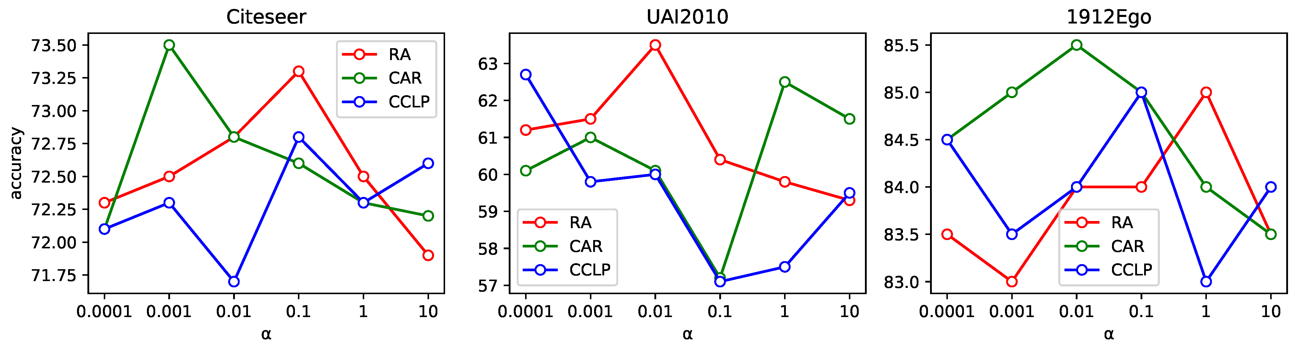
4.4. Hyperparameters

Table 5. The hyperparameters ($\lambda ,\alpha$) for optimal results.

	Cora	Citeseer	Pubmed	ACM
HS-GCN(RA)	5, 0.0001	0.5, 0.1	10, 0.01	5, 1
HS-GCN(CAR)	5, 0.1	0.5, 0.001	10, 1	5, 0.01
HS-GCN(CCLP)	5, 0.01	1, 0.1	5, 0.1	1, 0.0001
	UAI2010	414Ego	1912Ego	2106Ego
HS-GCN(RA)	0.5, 0.01	1, 1	0.5, 1	5, 0.001
HS-GCN(CAR)	0.5, 1	5, 1	0.5, 0.01	1, 0.0001
HS-GCN(CCLP)	0.5, 0.0001	1, 0.1	5, 0.1	1, 0.001

shows the values of the two hyperparameters corresponding to the experiments when they achieve the best results. It can be found that the optimal role of different node similarity methods has different weights ($\alpha$). For CCLP, its optimal weights are generally small (twice 0.0001 and all less than 1). As for the other two, $\alpha =1$ occurs 3 times for both.

It is also worth noting that there is consistency in the self-loop weights ($\lambda$) on the same dataset. This phenomenon is consistent with the intuition that the central nodes of the same dataset should have similar roles. For example, on dataset Pubmed, $\lambda$ tends to take large values (10, 10, 5), which indicates that the central nodes of Pubmed have high importance. For Citeseer and UAI2010, $\lambda$ tends to take small values, which indicates that neighborhood nodes have a greater impact on central nodes.

In addition, we take Citeseer, UAI2010 and 1912Ego as examples for parameter sensitivity analysis. Note that we are concerned about the influence of $\alpha$, for which $\lambda$ is controlled to take the corresponding optimal value (Give an example, when studying RA on Citeseer, we control $\lambda =0.5$, and then let $\alpha$ change and record the accuracy of the results).

As we can see in Figure 3, the fluctuations of accuracy are around 2% on Citeseer and 1912Ego. The fluctuation of accuracy on UAI2010 is much larger (about 6%), which means the results of UAI2010 are more sensitive to parameter $\alpha$. In addition, we can see that node similarity methods behave differently on each dataset. On dataset UAI2010, method RA is clearly superior among the three methods. For 1912Ego, the most dominant method is CAR. As for Citeseer, there is no clearly superior method.

5. Conclusions and Discussion

In this paper, we have designed a new framework combined with high-order node similarities – HS-GCN, which can exploit node similarities to mine the potential high-order structural features of graphs from different perspectives and effectively aggregate information from the nodes. We have analyzed theoretically that HS-GCN can be considered as a natural generalization of a series of convolution-based methods and conducted numerous experiments. The experimental results have shown that HS-GCN can effectively generate embeddings for nodes of unknown categories.

There are many extensions and potential improvements to our method, such as exploring more general methods of exploring node similarities or extending our method to more types of graphs.

References

1. Zeng, X.; Zhang, X.; Liao, Y.; Pan, L. Prediction and validation of association between microRNAs and diseases by multipath methods. Biochim. Biophys. Acta (BBA)-Gen. Subj. 2016, 1860, 2735–2739. [Google Scholar] [CrossRef] [PubMed]
2. Zhang, X.; Zeng, X. Integrative approaches for predicting microRNA function and prioritizing disease-related microRNA using biological interaction networks. Bio-Inspired Comput. Model. Algorithms 2019, 75–105. [Google Scholar]
3. Kandhway, K.; Kuri, J. Using node centrality and optimal control to maximize information diffusion in social networks. IEEE Trans. Syst. Man Cybern. Syst. 2016, 47, 1099–1110. [Google Scholar] [CrossRef] [Green Version]
4. Herzallah, R. Scalable Harmonization of Complex Networks with Local Adaptive Controllers. IEEE Trans. Syst. Man Cybern.-Syst. 2017, 47, 3. [Google Scholar]
5. Kipf, T.N.; Welling, M. Semi-Supervised Classification with Graph Convolutional Networks. In Proceedings of the 2017 International Conference on Learning Representations (ICLR), Toulon, France, 24–26 April 2017. [Google Scholar]
6. Choong, J.J.; Liu, X.; Murata, T. Learning community structure with variational autoencoder. In Proceedings of the 2018 IEEE International Conference on Data Mining (ICDM), Sentosa, Singapore, 17–20 November 2018; IEEE: New York, NY, USA, 2018; pp. 69–78. [Google Scholar]
7. Scarselli, F.; Gori, M.; Tsoi, A.C.; Hagenbuchner, M.; Monfardini, G. The graph neural network model. IEEE Trans. Neural Netw. 2008, 20, 61–80. [Google Scholar] [CrossRef] [Green Version]
8. Bruna, J.; Zaremba, W.; Szlam, A.; LeCun, Y. Spectral networks and locally connected networks on graphs. arXiv 2013, arXiv:1312.6203. [Google Scholar]
9. Defferrard, M.; Bresson, X.; Vandergheynst, P. Convolutional neural networks on graphs with fast localized spectral filtering. Adv. Neural Inf. Process. Syst. 2016, 29, 3844–3852. [Google Scholar]
10. Velickovic, P.; Cucurull, G.; Casanova, A.; Romero, A.; Lio, P.; Bengio, Y. Graph attention networks. Stat 2017, 1050, 20. [Google Scholar]
11. Niu, Z.; Zhong, G.; Yu, H. A review on the attention mechanism of deep learning. Neurocomputing 2021, 452, 48–62. [Google Scholar] [CrossRef]
12. Brauwers, G.; Frasincar, F. A General Survey on Attention Mechanisms in Deep Learning. IEEE Trans. Knowl. Data Eng. 2021. [Google Scholar] [CrossRef]
13. Hamilton, W.; Ying, Z.; Leskovec, J. Inductive representation learning on large graphs. Adv. Neural Inf. Process. Syst. 2017, 30. [Google Scholar]
14. Li, G.; Muller, M.; Thabet, A.; Ghanem, B. Deepgcns: Can gcns go as deep as cnns? In Proceedings of the 2019 IEEE/CVF International Conference on Computer Vision, Seoul, Republic of Korea, 27 October–2 November 2019; pp. 9267–9276. [Google Scholar]
15. Li, G.; Xiong, C.; Thabet, A.; Ghanem, B. Deepergcn: All you need to train deeper gcns. arXiv 2020, arXiv:2006.07739. [Google Scholar]
16. Xu, K.; Hu, W.; Leskovec, J.; Jegelka, S. How powerful are graph neural networks? arXiv 2018, arXiv:1810.00826. [Google Scholar]
17. Lv, X.; Wang, Z.L.; Ren, Y.; Yang, D.Z.; Feng, Q.; Sun, B.; Liu, D. Traffic network resilience analysis based on the GCN-RNN prediction model. In Proceedings of the 2019 International Conference on Quality, Reliability, Risk, Maintenance, and Safety Engineering (QR2MSE), Zhangjiajie, China, 6–9 August 2019; IEEE: New York, NY, USA, 2019; pp. 96–103. [Google Scholar]
18. Sun, M.; Zhao, S.; Gilvary, C.; Elemento, O.; Zhou, J.; Wang, F. Graph convolutional networks for computational drug development and discovery. Briefings Bioinform. 2020, 21, 919–935. [Google Scholar] [CrossRef]
19. Wang, X.; He, X.; Cao, Y.; Liu, M.; Chua, T.S. Kgat: Knowledge graph attention network for recommendation. In Proceedings of the 25th ACM SIGKDD International Conference on Knowledge Discovery and Data Mining, Anchorage, AK, USA, 4–8 August 2019; pp. 950–958. [Google Scholar]
20. Kosaraju, V.; Sadeghian, A.; Martín-Martín, R.; Reid, I.; Rezatofighi, H.; Savarese, S. Social-bigat: Multimodal trajectory forecasting using bicycle-gan and graph attention networks. Adv. Neural Inf. Process. Syst. 2019, 32. [Google Scholar]
21. Hamilton, W.L.; Ying, R.; Leskovec, J. Representation learning on graphs: Methods and applications. arXiv 2017, arXiv:1709.05584. [Google Scholar]
22. Xia, F.; Sun, K.; Yu, S.; Aziz, A.; Wan, L.; Pan, S.; Liu, H. Graph learning: A survey. IEEE Trans. Artif. Intell. 2021, 2, 109–127. [Google Scholar] [CrossRef]
23. Wang, S.; Hu, L.; Wang, Y.; He, X.; Sheng, Q.Z.; Orgun, M.A.; Cao, L.; Ricci, F.; Yu, P.S. Graph learning based recommender systems: A review. arXiv 2021, arXiv:2105.06339. [Google Scholar]
24. Jepsen, T.S.; Jensen, C.S.; Nielsen, T.D. Relational Fusion Networks: Graph Convolutional Networks for Road Networks. IEEE Trans. Intell. Transp. Syst. 2022, 23, 418–429. [Google Scholar] [CrossRef]
25. Dong, Y.; Liu, Q.; Du, B.; Zhang, L. Weighted feature fusion of convolutional neural network and graph attention network for hyperspectral image classification. IEEE Trans. Image Process. 2022, 31, 1559–1572. [Google Scholar] [CrossRef]
26. Kumar, A.; Singh, S.S.; Singh, K.; Biswas, B. Link prediction techniques, applications, and performance: A survey. Phys. A Stat. Mech. Its Appl. 2020, 553, 124289. [Google Scholar] [CrossRef]
27. Adamic, L.A.; Adar, E. Friends and neighbors on the web. Soc. Netw. 2003, 25, 211–230. [Google Scholar] [CrossRef] [Green Version]
28. Barabási, A.L.; Albert, R. Emergence of scaling in random networks. Science 1999, 286, 509–512. [Google Scholar] [CrossRef] [PubMed] [Green Version]
29. Ravasz, E.; Somera, A.L.; Mongru, D.A.; Oltvai, Z.N.; Barabási, A.L. Hierarchical Organization of Modularity in Metabolic Networks. Science 2002, 297, 1551–1555. [Google Scholar] [CrossRef] [Green Version]
30. Dong, Y.; Ke, Q.; Wang, B.; Wu, B. Link Prediction Based on Local Information. In Proceedings of the 2011 International Conference on Advances in Social Networks Analysis and Mining, Kaohsiung, Taiwan, 25–27 July 2011; pp. 382–386. [Google Scholar]
31. Katz, L. A new status index derived from sociometric analysis. Psychometrika 1953, 18, 39–43. [Google Scholar] [CrossRef]
32. Lorrain, F.; White, H.C. Structural equivalence of individuals in social networks. J. Math. Sociol. 1971, 1, 49–80. [Google Scholar] [CrossRef]
33. Salton, G.; McGill, M.J. Introduction to Modern Information Retrieval; Mcgraw-Hill: New York, NY, USA, 1983; p. 448. [Google Scholar]
34. Sorensen, T. A method of establishing groups of equal amplitude in plant sociology based on similarity of species content, and its application to analyses of the vegetation on Danish commons. K. Dan. Vidensk. Selsk. Skr. 1948, 5, 1–34. [Google Scholar]
35. Leicht, E.A.; Holme, P.; Newman, M.E.J. Vertex similarity in networks. Phys. Rev. E 2006, 73, 026120. [Google Scholar] [CrossRef] [Green Version]
36. Zhou, T.; Lü, L.; Zhang, Y.C. Predicting missing links via local information. Eur. Phys. J. B 2009, 71, 623–630. [Google Scholar] [CrossRef] [Green Version]
37. Cannistraci, C.V.; Alanis-Lobato, G.; Ravasi, T. From link-prediction in brain connectomes and protein interactomes to the local-community-paradigm in complex networks. Sci. Rep. 2013, 3, 1–14. [Google Scholar] [CrossRef] [PubMed] [Green Version]
38. Wu, Z.; Lin, Y.; Wang, J.; Gregory, S. Link prediction with node clustering coefficient. Phys. A Stat. Mech. Its Appl. 2016, 452, 1–8. [Google Scholar] [CrossRef] [Green Version]
39. Klicpera, J.; Bojchevski, A.; Günnemann, S. Predict then propagate: Graph neural networks meet personalized pagerank. arXiv 2018, arXiv:1810.05997. [Google Scholar]
40. Milo, R.; Shen-Orr, S.; Itzkovitz, S.; Kashtan, N.; Chktovskii, D.; Alan, U. Network Motifs: Simple Building Blocks of Complex Networks. Science 2011, 298, 824–827. [Google Scholar] [CrossRef]
41. Aktas, M.E.; Nguyen, T.; Jawaid, S.; Riza, R.; Akbas, E. Identifying critical higher-order interactions in complex networks. Sci. Rep. 2021, 11, 21288. [Google Scholar] [CrossRef] [PubMed]
42. Wang, X.; Ji, H.; Shi, C.; Wang, B.; Ye, Y.; Cui, P.; Yu, P.S. Heterogeneous Graph Attention Network. In Proceedings of the 2019 The World Wide Web Conference, San Francisco, CA, USA, 13–17 May 2019; pp. 2022–2032. [Google Scholar]
43. Wang, W.; Liu, X.; Jiao, P.; Chen, X.; Jin, D. A Unified Weakly Supervised Framework for Community Detection and Semantic Matching. In Proceedings of the 2018 Advances in Knowledge Discovery and Data Mining, Melbourne, VIC, Australia, 3–6 June 2018; pp. 218–230. [Google Scholar]
44. Wang, X.; Zhu, M.; Bo, D.; Cui, P.; Shi, C.; Pei, J. Am-gcn: Adaptive multi-channel graph convolutional networks. In Proceedings of the 26th ACM SIGKDD International Conference on Knowledge Discovery & Data Mining, Virtual Event, 6–10 July 2020; pp. 1243–1253. [Google Scholar]
45. McAuley, J.; Leskovec, J. Learning to Discover Social Circles in Ego Networks. In Proceedings of the 25th International Conference on Neural Information Processing Systems (NIPS’12), Lake Tahoe, NV, USA, 3–6 December 2012; Volume 1, pp. 539–547. [Google Scholar]
46. Perozzi, B.; Al-Rfou, R.; Skiena, S. Deepwalk: Online learning of social representations. In Proceedings of the 20th ACM SIGKDD International Conference on Knowledge Discovery and Data Mining, New York, NY, USA, 24–27 August 2014; pp. 701–710. [Google Scholar]
47. Grover, A.; Leskovec, J. node2vec: Scalable feature learning for networks. In Proceedings of the 22nd ACM SIGKDD International Conference on Knowledge Discovery and Data Mining, San Francisco, CA, USA, 13–17 August 2016; pp. 855–864. [Google Scholar]
48. Weisfeiler, B.Y.; Leman, A.A. A reduction of a Graph to a Canonical Form and an Algebra Arising during this Reduction. Nauchno-Tech. Inf. 1968, 2, 12–16. [Google Scholar]
Figure 1. An example for CCLP, where S C C L P ( a , b ) > S C C L P ( e , f ) .
Mathematics 10 04586 g001
Figure 2. Overview of the HS-GCN process. Subfigure (A): high-order structural information is collected through high-order similarity method; Subfigures (BD): graph convolution operations are performed on the weighted graph.
Mathematics 10 04586 g002
Figure 3. Parameter sensitivity analysis on Citeseer, UAI2010 and 1912Ego. The x-axis is the values of α , and the y-axis represents the accuracy (max%).
Mathematics 10 04586 g003