Solitary Wave Interactions with an External Periodic Force: The Extended Korteweg-de Vries Framework

Abstract

In this work we asymptotically and numerically studied the interaction of large amplitude solitary waves with an external periodic force using the forced extended Korteweg-de Vries equation (feKdV). Regarding these interactions, we found three types of regimes depending on the amplitude of the solitary wave and how its speed and the speed of the external force are related. A solitary wave can remain steady when its crest and the crest of the external force are in phase, it can bounce back and forth remaining close to its initial position when its speed and the external force speed are near resonant, or it can move away from its initial position without reversing its direction. Additionally, we verified that the numerical results agreed qualitatively well within the asymptotic approximation theory for external broad forces.

1. Introduction

Solitary wave interactions with an external force is a topic of great interest that has been studied extensively over the last decades. The external force typically models a localized topography or a moving source that propagates along the free surface wave [1]. The main framework considered to study such interactions, and perhaps also the simplest, is the forced Korteweg-de Vries equation (fKdV) [2,3,4,5,6,7,8]. However, in recent years these interactions have been investigated in different frameworks such as the Euler equations [9], the forced modified Korteweg-de Vries equation (mKdV) [10] and the non-integrable forced Whitham equation [11,12]. An interesting phenomenon that occurs during these interactions is called trapped waves, which are described as waves that bounce back and forth at the external force remaining trapped for large times. This phenomenon occurs when the speed of the solitary wave and the external force are almost in resonance.

A complete asymptotic study on trapped waves for the fKdV equation was done by Grimshaw and collaborators for a localized external force [13,14]. Three types of regimes were identified in the asymptotic framework. A solitary wave can bounce back and forth at the external force remaining trapped for large times, it can pass over the external force without reversing its direction, or it remains steady at the external force. Besides, in these works, the authors found that the results within the developed asymptotic framework agreed well with the numerical predictions. Regarding an external periodic force, differently from the localized external force, radiation is spontaneously generated all over the domain. This raises a natural problem, which is to describe what waves are actually produced due to the interaction between the solitary wave and the external force or just radiation due to a non-localized external force. In order to address this issue, Malomed [15] proposed a change of variables to separate these two types of generated waves and investigated the emission of radiation of solitons in the presence of an external periodic force in the fKdV equation framework asymptotically. He showed that the external force does not capture the solitons. In fact, under the action of the radiative losses, a soliton that was moving slower than the external force is further decelerated, while the one which was faster is accelerated. Numerical results confirming his findings were reported later by Grimshaw et al. [16].

Although the fKdV is widely used as a first approximation to study many nonlinear phenomena, when solitons have a larger amplitude or the nonlinearity is more dominant in the wave propagation phenomenon, nonlinear terms of higher-order have to be considered. In that case, the forced extended KdV equation (eKdV) or the forced Gardner equation gives rise. This equation incorporates a quadratic and cubic nonlinearity. Among the problems that can be investigated in this framework, we mention internal waves in two-layer fluids. In this particular case, the sign of the cubic term depends on the oceanic stratification. Although the eKdV equation is integrable, the nonlinear dynamics are more complicated than the fKdV equation and the sign of cubic nonlinearity plays a fundamental role in the qualitative behavior of the solutions. For instance, the eKdV equation is more interesting than the fKdV equation in the sense that it describes various types of wave solutions—not just solitons. The eKdV admits as solutions, for instance, solitons of both polarities, breathers (traveling oscillating moving wave packets) and dissipationless shock waves. Focusing on trapped waves, Grimshaw and Pelinovsky [17] derived a second-order nonlinear dynamical system for the amplitude and the crest position of the soliton to study the interaction of the soliton and a localized external force. Besides, conditions for capturing or repulsion of a soliton by an external force were obtained. However, to the best of our knowledge there are no articles with the forced eKdV studying trapped waves in the presence of a external periodic wave field.

In this article, differently from the mentioned works above, we focus on the interaction of solitary waves with a periodic external force in the forced eKdV equation framework.

The outline of the present article is as follows. In Section 2 we introduce the forced eKdV equation. The asymptotic and numerical results are presented in Section 3. The discussion and conclusions in are presented in Section 4 and Section 5, respectively.

2. The Forced Extended Korteweg-de Vries Equation

We consider the extended Korteweg-de Vries equation in the canonical form with an external force term as the model to study the trapped waves

$$U_t+6U{U}_x+U^2{U}_x+U_{xxx}=ϵf_x(x+\Delta t),$$

(1)

where $U(x,t)$ is the surface wave profile, $f(x+\Delta t)$ is the external periodic force that travels with constant speed $\Delta$, and $ϵ>0$ is a small parameter. It is convenient to rewrite Equation (1) in the external force moving frame. Therefore,

$$U_t+\Delta U_x+6U{U}_x+U^2{U}_x+U_{xxx}=ϵf_x\left(x\right).$$

(2)

This equation conserves mass $\left(M\right(t\left)\right)$, with

$$\frac{dM}{dt}=0,\mathrm{where} M\left(t\right)={\int }_{-\infty }^{\infty }U(x,t)dx,$$

(3)

and the rate of change of momentum $\left(P\right(t\left)\right)$ is balanced by the external force as

$$\frac{dP}{dt}={\int }_{-\infty }^{\infty }U(x,t)\frac{df\left(x\right)}{dx}dx,\mathrm{where} P\left(t\right)=\frac{1}{2}{\int }_{-\infty }^{\infty }{U}^2(x,t)dx.$$

(4)

In the absence of an external force, the eKdV admits two families of solitary waves as solutions [18], which are given by the expressions

$$U(x,t)=\frac{{\gamma }^2}{1+Bcosh\left(\gamma \right(x-ct\left)\right)},\mathrm{where} c=\Delta +{\gamma }^2,B^2=1+\frac{{\gamma }^2}{6}.$$

(5)

Here we only analyze elevation solitary waves ($B>0$), whose amplitude is

$$a=\frac{{\gamma }^2}{1+B}=6(B-1).$$

(6)

The external periodic force is modeled by the function

$$f\left(x\right)=Asin\left(qx\right),$$

(7)

where A is its amplitude and q is the wave number. Since the perturbation f is not localized, it produces radiation all over the domain, even far away from where most of the energy of the solitary wave is localized. Although it does not affect the asymptotic study at the lowest orders, it can be troublesome for the numerical study. For this reason, we use a similar trick as done by Malomed [15]. Inserting into Equation (2)

$$U(x,t)=u(x,t)+ϵu_0\left(x\right),$$

where

$$u_0\left(x\right)=\frac{A}{\Delta -q^2}sin\left(qx\right)$$

is the solution of the linearized feKdV Equation (2), we have that $u(x,t)$ satisfies

$$u_t+6u{u}_x+u^2{u}_x+u_{xxx}=-6ϵ{\left(u_{0}u\right)}_x-ϵ{\left(u^2{u}_0\right)}_x+\mathcal{O}\left({ϵ}^2\right).$$

Consequently, at first approximation, we obtain the new equation

$$u_t+6u{u}_x+u^2{u}_x+u_{xxx}=-6ϵ{\left(u_{0}u\right)}_x-ϵ{\left(u^2{u}_0\right)}_x,$$

(8)

where the perturbation is now localized along the free surface $u(x,t)$.

3. Results

3.1. Asymptotic Theory

In this section we introduce the asymptotic theory that allows to turn the study of the partial differential Equation (2) into a dynamical system. This idea has been used in different contexts [13,14]; in particular for the interest reader we mention the recent works of Frassu and Viglialoro [19] and Frassu et al. [20], where the authors analyze dynamical systems modeling chemotaxis mechanisms formulated through partial differential equations.

Asymptotic results on the interaction of a solitary wave with an external force were first reported by Grimshaw and Pelinovsky [17]. For the sake of completeness, we recall their main results assuming that $f\left(X\right)\to 0$ as $\left|X\right|\to \infty$. For a weak external force ($ϵ\ll 1$), we seek for a slowly time-varying solitary wave with expansion

$$\begin{array}{c}\hfill \begin{array}{cc}\hfill & U(x,t)=U_0(\xi ,t)+ϵU_1+\cdots ,\hfill \\ \hfill & \xi =x-X\left(t\right),\hfill \end{array}\end{array}$$

(9)

where $X\left(t\right)$ is the position of the crest of the wave. At first order, the wave profile is given by

$$\begin{array}{c}\hfill \begin{array}{cc}\hfill & U(\xi ,t)=\frac{{\gamma }^2}{1+Bcosh\left(\gamma \xi \right)},\hfill \\ \hfill & \frac{dX}{dt}=c=\Delta +{\gamma }^2.\hfill \end{array}\end{array}$$

(10)

In particular, the amplitude variation as a function of time can be obtained from the first-order momentum Equation (4)

$$P_0\left(t\right)=\frac{1}{2}{\int }_{-\infty }^{\infty }{U}_0^2(\xi ,t)d\xi ,$$

(11)

and its rate of change at first-order, which is given by

$$\frac{d{P}_0}{dt}={\int }_{-\infty }^{\infty }{U}_0(x-X\left(t\right))\frac{df\left(x\right)}{dx}dx.$$

(12)

Notice that $P_0$ is a function of $\gamma \left(t\right)$, thus the dynamical system (10)–(12) describes the amplitude and the position of the crest of the solitary wave solution. Assuming a broad external force, the momentum equations reads

$$\frac{d{P}_0}{dt}=M_0\frac{df\left(X\right)}{dX},\mathrm{where} M_0={\int }_{-\infty }^{\infty }{U}_0(\xi ,t)d\xi .$$

(13)

Moreover, in the weak-amplitude solitary wave regime ($a\ll 1$), the quantities $M_0$, $P_0$, $\gamma$ can be obtained in explicit form

$$M_0=2\sqrt{2}{a}^{1/2},P_0=\frac{2\sqrt{2}}{3}{a}^{3/2},{\gamma }^2=2a.$$

(14)

Therefore, the dynamical system for the amplitude and position of the crest is

$$\begin{array}{c}\hfill \begin{array}{cc}\hfill & \frac{dX}{dt}=\Delta +2a.\hfill \\ \hfill & \frac{da}{dt}=2\frac{df\left(X\right)}{dX}.\hfill \end{array}\end{array}$$

(15)

From Equation (15) we have that the position of the crest of a solitary wave is described by the oscillator

$$\begin{array}{c}\hfill \begin{array}{cc}\hfill & \frac{d^{2}X}{d{t}^2}=4\frac{df\left(X\right)}{dX}.\hfill \end{array}\end{array}$$

(16)

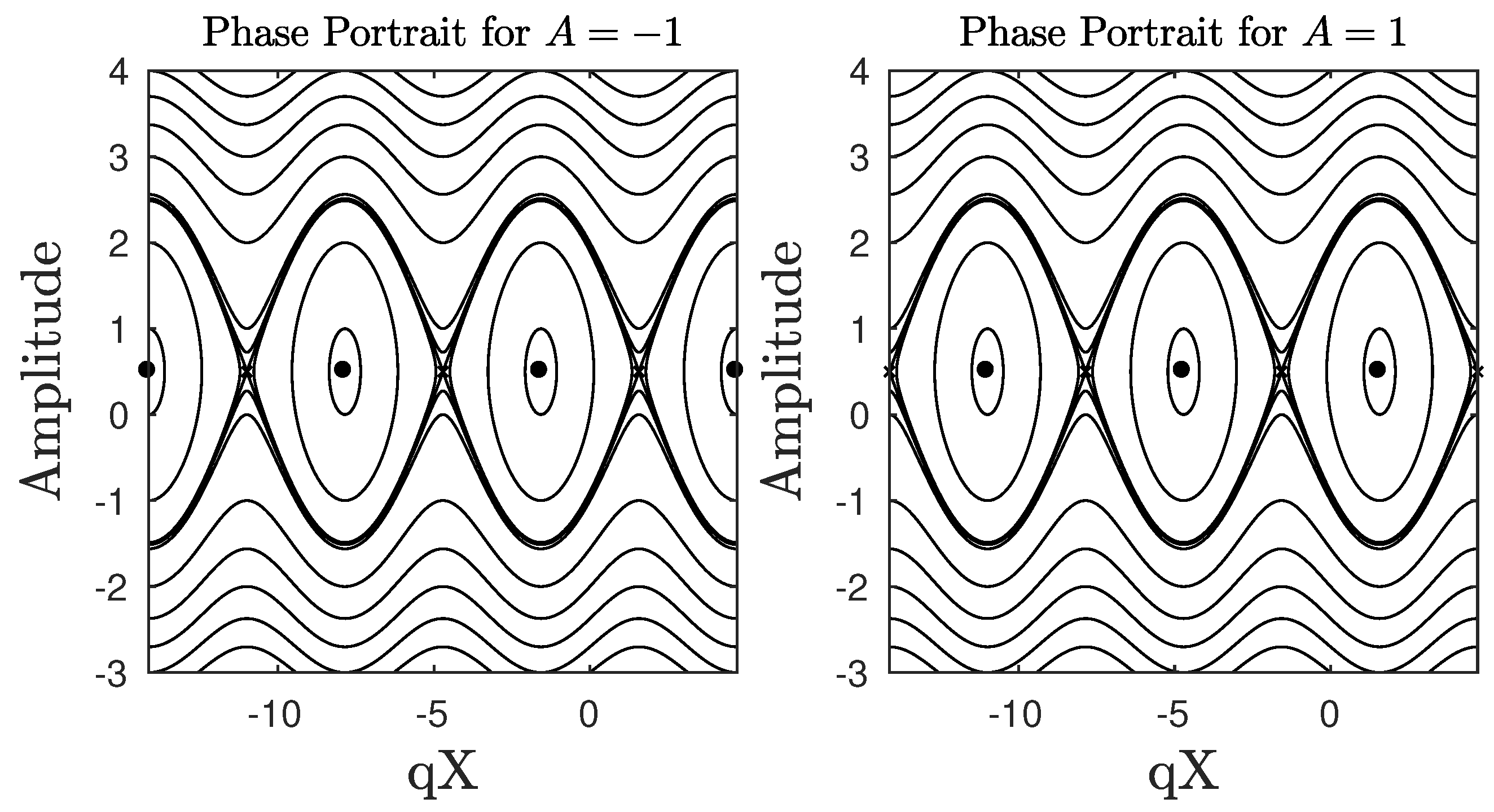
Here, we formally consider the periodic external force to be as the one defined in Equation (7). In fact, if the external force is broad in comparison with the soliton length, the asymptotic theory is valid for any function $f\left(X\right)$—not only with vanishing ends. It works for periodic external forces with small values of q. It can be shown that the equilibrium points of this dynamical system are $x=\pi /2q+k\pi$, where k is an integer. Centers occur aligned with the crests of the external force while saddles are aligned with the troughs of the external force. Consequently, as we change the sign of A, the centers become saddles and vice-versa. It is worth to mention that centers and saddles represent solitary waves that remain steady for all times, a closed orbit represents a trapped solitary wave, and a non-closed orbit corresponds to a solitary wave that propagates without reversing its direction. Therefore, a phase-portrait of the dynamical system (15) qualitatively describes the behavior of the solitary wave and the external force interaction except for small corrections (order $\mathcal{O}\left(ϵ\right)$).

Solutions of the dynamical system (15) are represented by streamlines i.e., solutions are the level curves of the stream function $H(X,a)$, which is given by

$$H(X,a)=-2f\left(X\right)+\Delta a+a^2.$$

(17)

Figure 1 displays the typical phase portraits of the dynamical system (15). We recall that a closed orbit illustrates a solitary wave that is trapped with no radiation due to its interaction with the external force while a non-closed orbit represents a solitary wave that propagates without reversing its direction. It is worth to mention that in Figure 1 (left) each center is aligned with a crest of the external force while in Figure 1 (right) each center is aligned with a trough of the external force. Although the asymptotic results presented here are limited to the weak-amplitude case, as it follows from Grimshaw and Pelinovsky [17], qualitative results still hold for arbitrary amplitudes of the solitary waves and we do not reproduce them here.

3.2. Numerical Results

Equation (8) is solved numerically in a periodic computational domain $[-L,L]$ with a uniform grid with N points using a Fourier pseudospectral method with an integrating factor [21]. The computational domain is taken large enough in order to prevent effects of the spatial periodicity. The time evolution is calculated through the Runge–Kutta fourth-order method with time step $\Delta t$. Typical computations are performed using $N=2^{12}$ Fourier modes $L=512$ and $\Delta t={10}^{-3}$ in MATLAB. In order to verify the accuracy of the numerical solutions, simulations are compared using a different number of Fourier modes ($2^{13}$ and $2^{14}$), and the results are the same. A study of the resolution of a similar numerical method can be found in Ref. [7].

In order to compare the numerical solutions with the asymptotic predictions, we verify whether the equilibrium points of a dynamical system (15) represent qualitative solutions of Equation (8). In other words, we verify if a point near a saddle point represents a solitary wave that travels without reversing its direction and if a center point corresponds to a trapped solitary wave. Since there is a long list of parameters to be considered in the study of the interaction between a solitary wave and the external force (7), we fix a few parameters, namely, $ϵ=0.01$, $A=-1$, $\gamma =1$ and $q=(\pi /L)n$, where n is an integer, which represents the number of waves in the interval $[-L,L]$. Thus, large values of n represent high frequencies while small values of n represent low frequencies. Notice that with these choices of parameters, the initial solitary wave has amplitude $\left(a\right)$, as defined in Equation (6). Additionally, the initial solitary waves are chosen to be with their crests located at $x=x_0$, where $x_0=\pm \pi /2q$. We recall that according to the dynamical system (15), choosing $\Delta =-2a$ and the position of crest $x_0=+\pi /2q$, we have a saddle, and by choosing $\Delta =-2a$ and the position of crest $x_0=-\pi /2q$, we obtain a center.

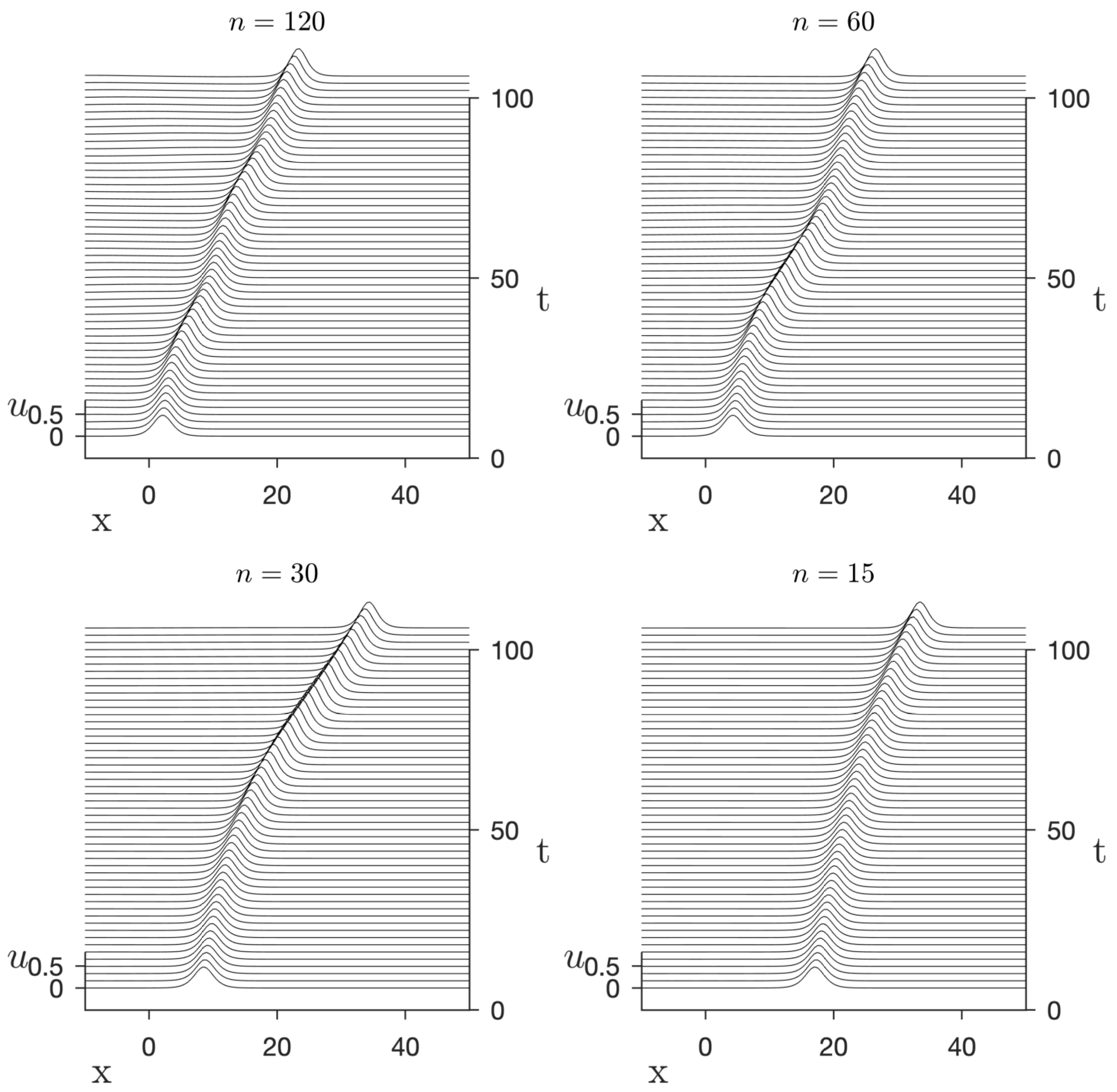
Firstly, we consider the simplest case—the saddle points. To this end, we run a large number of simulations and observe that the solitary waves move past the external force without changing their directions. However, reflection is observed as a solitary wave pass over multiple bumps. The reflection decreases as the frequency of the external force increases, which causes a change in the amplitude of the solitary waves. 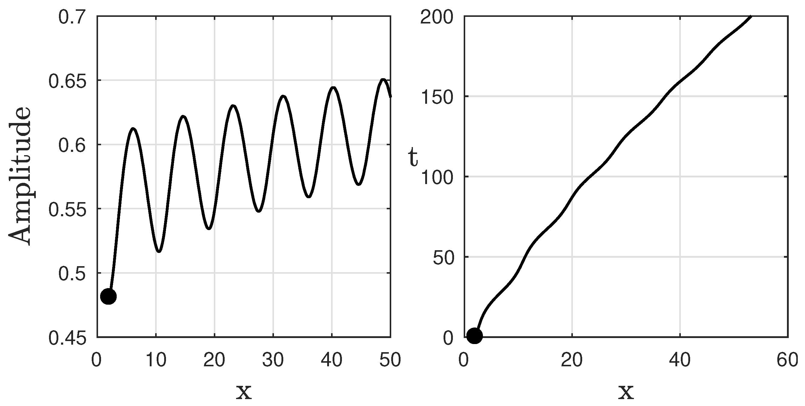This typical behavior is illustrated in Figure 2 for different values of the parameter n. Details of the variations in the amplitude of the solitary wave for the case $n=120$ are given in Figure 3. Notice that the amplitude of the solitary wave oscillates as it passes over each bump of the external force (see Figure 3 (left)). Additionally, the solitary wave speed keeps oscillating in time due to the interaction with the external force as displayed in Figure 3 (right). This dynamic is qualitatively represented by the non-closed orbits of the dynamical system (15), see Figure 1 (left). In fact, the fully numerical simulations and the dynamical system agree quantitatively well for small times. To see this, we recall that the asymptotic theory is obtained by truncating the terms of Equation (9) at order $\mathcal{O}\left(ϵ\right)$ which is the same order of the amplitude variations depicted in Figure 3 (left).

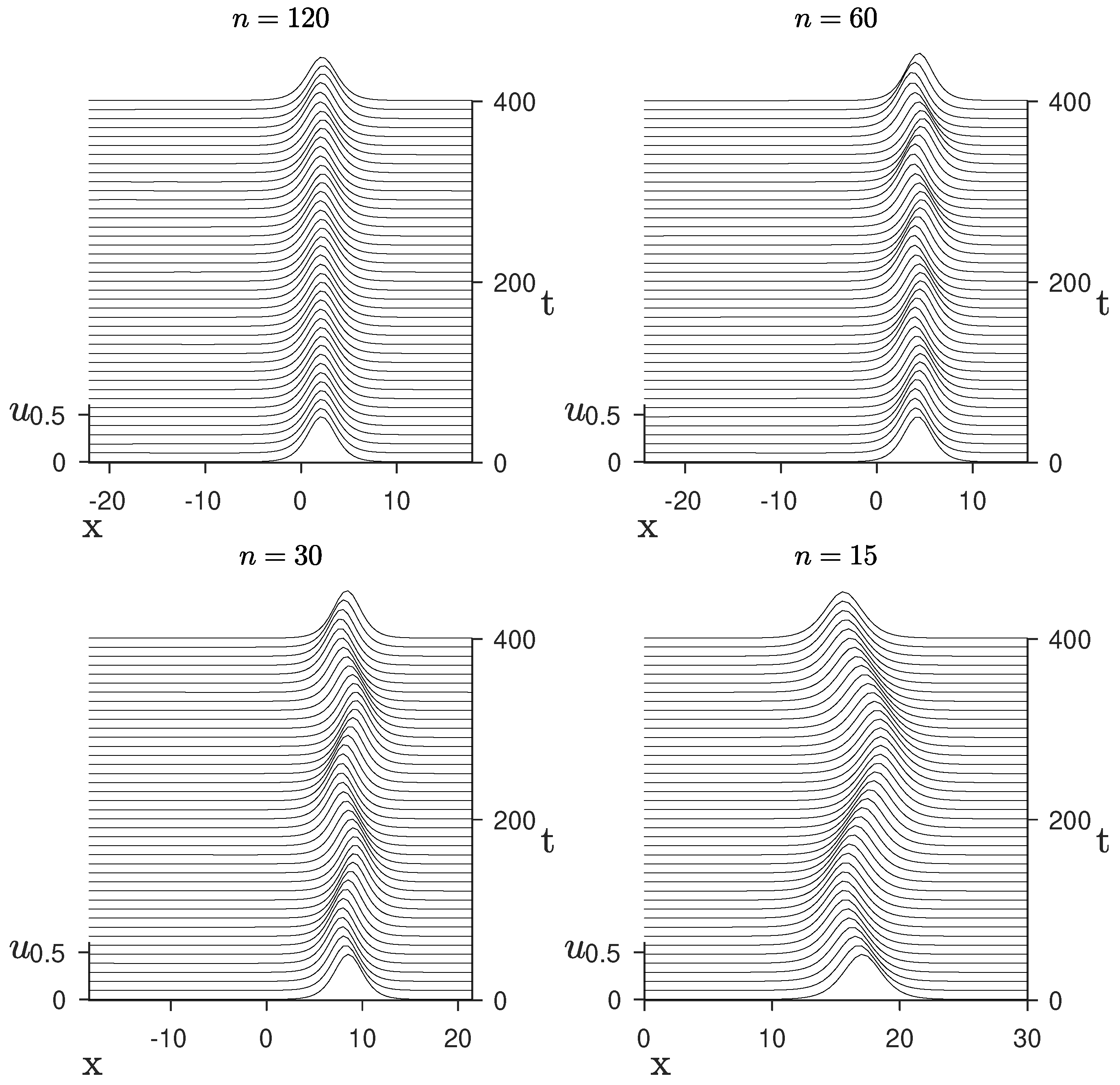
Now, we investigate if the center points of the dynamical system (15) define trapped waves for Equation (8). So, we let q vary and compare the numerical results within the asymptotic framework. For large values of n, a solitary wave barely feels the external force, consequently the solitary wave remains almost steady, resembling the equilibrium center point of the dynamical system (15). 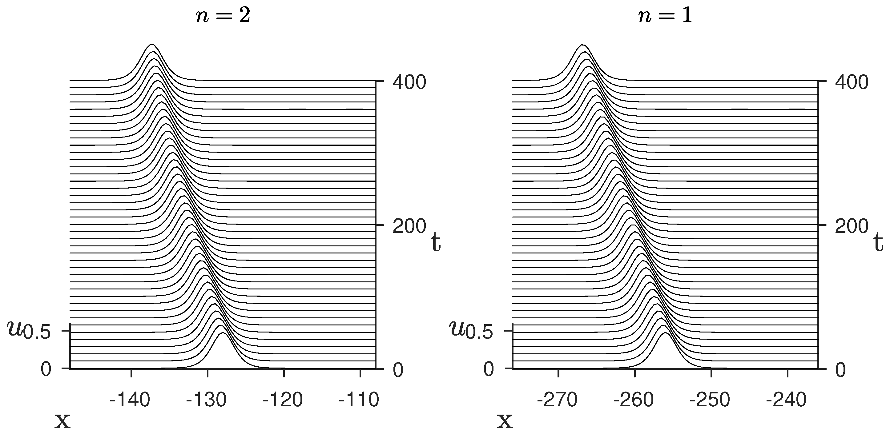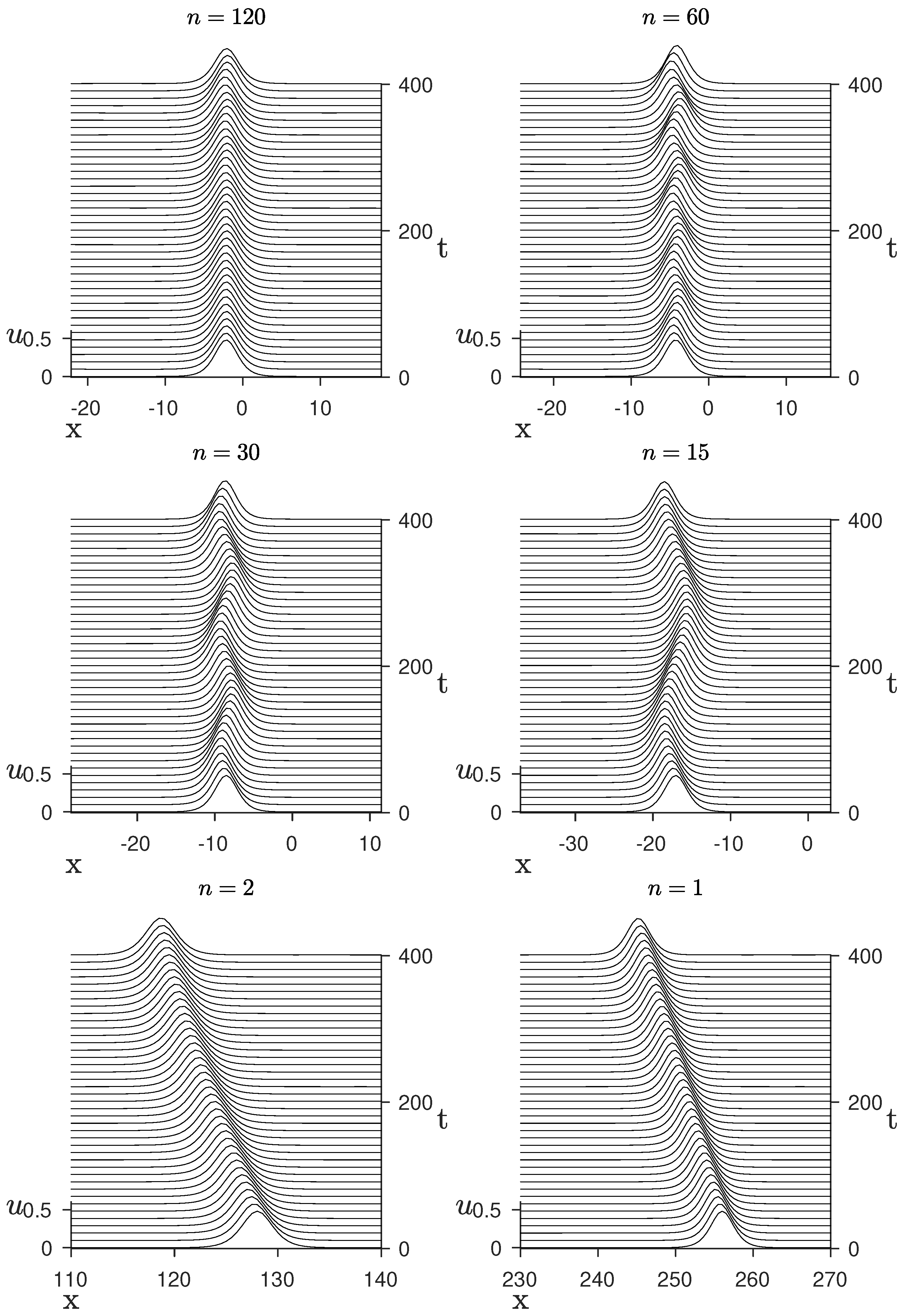As we decrease the values of n, for instance $n=120,60,30,15$ the solitary wave bounces back and forth close to its initial position for large times with little radiation being emanated. These results are in agreement with the ones predicted by the asymptotic theory and are illustrated in Figure 4. 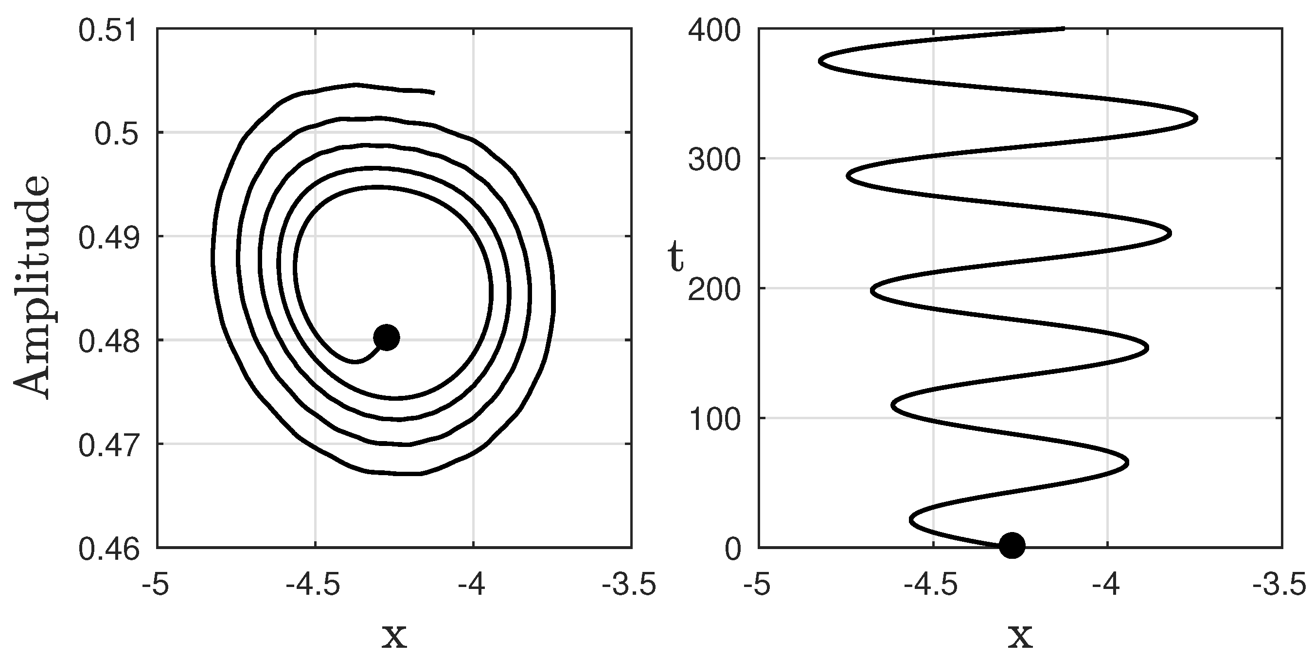We observe that large values of the parameter n lead to small oscillations of the crest-position of the solitary wave, i.e., the larger n is the closest the solitary wave remains to its initial position. In Figure 5 (left) we display the amplitude vs. crest of the solitary wave position and its crest position along time is shown in Figure 5 (right) for $n=60$. Notice that the amplitude dynamics in the amplitude vs. crest position phase resembles an unstable spiral. Meanwhile, we observe that the crest position oscillates by increasing in time. This indicates that the solitary wave might move away from its initial position. It worth to mention that it does not contradict the predictions of the asymptotic theory since both theories are only expected to agree well at small times. It is noteworthy that for small perturbations of $\Delta =-2a$, the solitary waves still remain trapped close to their initial positions for large times. In particular, it shows that the asymptotic theory for a broad external force in the weak-amplitude solitary wave regime gives good results qualitatively.

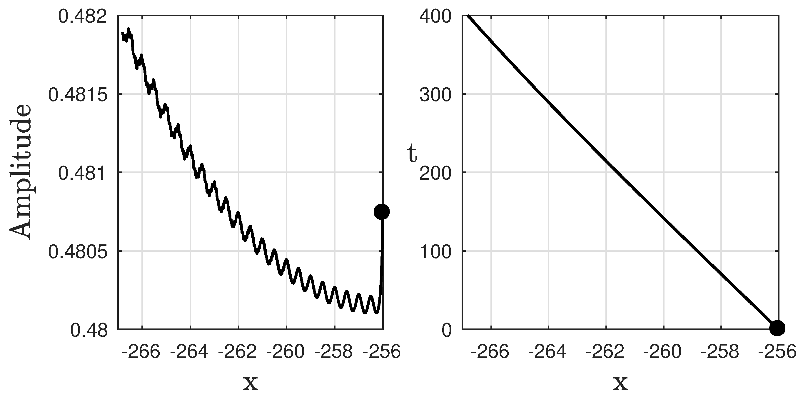
When n is small, numerical results differ from the asymptotic theory. In fact, the asymptotic method breaks for small values of q. It occurs because for too small values of q the forcing is proportional to ${ϵ}^2$. Therefore, the solitary waves are not affected by the external force. Figure 6 displays the evolution of two solitary waves for small values of n. Notice that the solitary wave propagates to the left without reversing its direction. Moreover, the change in amplitude of these solitary waves is small (see Figure 7 (left)) and the solitary wave speed is almost constant, as depicted in Figure 7 (right). Initially, the amplitude of the solitary wave is adjusted to the external force and later it changes only slightly. Consequently, the solitary wave travels almost as a classical solitary wave solution of the unforced problem (1).

It is worth to mention that similar results are observed for positive choices of the amplitude of the external force $\left(A\right)$. To illustrate this, we limit ourselves to show Figure 8. As we compare the respective panels of Figure 4 and Figure 8 we see that they are all the same unless translations.

4. Discussion

The results presented here complement the series of studies that have been done in the literature for localized external forces. This work can be extended to several other equations such as the forced mKdV equation, Schamel equation and even to the non-integrable family of Whitham equations, which has been a trend in the past few years, especially from a theoretical point of view. Although we have considered only spatial periodic external fields, time-dependent fields can also be considered and the dynamics should be more interesting. Additionally, even though we did not focus on the applicability of the results discussed in this article, it can be interpreted not only in water waves theory, but also in other branches of physics for example, surface waves in electric normal fields and atmospheric waves and elastic waves in solids, which makes our study to be urgent.

5. Conclusions

In this paper, we have asymptotically and numerically investigated the interaction between solitary waves and an external periodic force within the feKdV equation. We found that a solitary wave can remain steady if its amplitude and crest position are chosen accordingly, as it can bounce back and forth close to its initial position or it can simply move away from its initial positions. These results agree qualitatively within the asymptotic theory considering a broad external force when compared with the length of the solitary wave. However, when the wavenumber of the periodic forcing is too small, the asymptotic fails because solitary waves are trapped longer within the eKdV equation.

References

1. Baines, S. Topographic Effects in Stratified Flows; Cambridge University Press: Cambridge, UK, 1995. [Google Scholar]
2. Lee, S.; Whang, S. Trapped supercritical waves for the forced KdV equation with two bumps. Appl. Math. Model. 2015, 39, 2649–2660. [Google Scholar] [CrossRef]
3. Lee, S. Dynamics of trapped solitary waves for the forced KdV equation. Symmetry 2018, 10, 129. [Google Scholar] [CrossRef] [Green Version]
4. Kim, H.; Choi, H. A study of wave trapping between two obstacles in the forced Korteweg-de Vries equation. J. Eng. Math. 2018, 108, 197–208. [Google Scholar] [CrossRef]
5. Ermakov, A.; Stepanyants, Y. Soliton interaction with external forcing within the Korteweg-de Vries equation. Chaos 2019, 29, 013117. [Google Scholar] [CrossRef] [PubMed] [Green Version]
6. Flamarion, M.V.; Ribeiro, R., Jr. Solitary water wave interactions for the Forced Korteweg-de Vries equation. Comp. Appl. Math. 2021, 40, 312. [Google Scholar] [CrossRef]
7. Flamarion, M.V.; Ribeiro, R., Jr. Gravity-capillary flows over obstacles for the fifth-order forced Korteweg-de Vries equation. J. Eng. Math. 2021, 129, 1–17. [Google Scholar] [CrossRef]
8. Flamarion, M.V. Generation of trapped depression solitary waves in gravity-capillary flows over an obstacle. Comp. Appl. Math. 2022, 41, 31. [Google Scholar] [CrossRef]
9. Flamarion, M.V.; Ribeiro, R., Jr. Trapped solitary-wave interaction for Euler equations with low-pressure region. Comp. Appl. Math. 2021, 40, 20. [Google Scholar] [CrossRef]
10. Flamarion, M.V.; Pelinovsky, E. Soliton interactions with an external forcing: The modified Korteweg-de Vries framework. Chaos Solitons Fractals 2022, 165, 112889. [Google Scholar] [CrossRef]
11. Flamarion, M.V. Waves generated by a submerged topography for the Whitham equation. Int. J. Appl. Comput. Math. 2022, 8, 257. [Google Scholar] [CrossRef]
12. Flamarion, M.V. Trapped waves generated by an accelerated moving disturbance for the Whitham equation. Partial. Differ. Equ. Appl. Math. 2022, 5, 100356. [Google Scholar] [CrossRef]
13. Grimshaw, R.; Pelinovsky, E.; Tian, X. Interaction of a solitary wave with an external force. Phys. D 1994, 77, 405–433. [Google Scholar] [CrossRef]
14. Grimshaw, R.; Pelinovsky, E.; Pavel, S. Interaction of a solitary wave with an external force moving with variable speed. Stud. Appl. Math. 1996, 142, 433–464. [Google Scholar]
15. Malomed, B.A. Emission of radiation by a KdV soliton in a periodic forcing. Phys. Lett. A 1993, 172, 373–377. [Google Scholar] [CrossRef]
16. Grimshaw, R.; Malomed, B.A.; Tian, X. Dynamics of a KdV soliton due to periodic forcing. Phys. Lett. A 1993, 179, 291–298. [Google Scholar] [CrossRef]
17. Grimshaw, R.; Pelinovsky, E. Interaction of a solitary wave with an external force in the extended Korteweg-de Vries equation. Int. J. Bifurcat. Chaos 2002, 12, 2409–2419. [Google Scholar] [CrossRef]
18. Grimshaw, R.; Pelinovsky, E.; Talipova, T.; Kurkina, O. Internal solitary waves: Propagation, deformation and disintegration. Nonlinear Process. Geophys. 2010, 17, 633–649. [Google Scholar] [CrossRef] [Green Version]
19. Frassu, S.; Viglialoro, G. Boundedness criteria for a class of indirect (and direct) chemotaxis- consumption models in high dimensions. Appl. Math. Lett. 2022, 132, 108108. [Google Scholar] [CrossRef]
20. Frassu, S.; Galván, R.R.; Viglialoro, G. Uniform in time L-estimates for an attraction-repulsion chemotaxis model with double saturation. Discret. Contin. Dyn. Syst.-B 2023, 28, 1886–1904. [Google Scholar] [CrossRef]
21. Trefethen, L.N. Spectral Methods in MATLAB; SIAM: Philadelphia, PA, USA, 2001. [Google Scholar]
Figure 1. Phase portraits for the dynamical system (15) for Δ = 1 . Circles correspond to centers and crosses to saddles of the dynamical system (15).
Mathematics 10 04538 g001
Figure 2. Solitary wave solutions over the periodic forcing. Parameters: Δ = 2 a , x 0 = + π / 2 q , A = 1 .
Mathematics 10 04538 g002
Figure 3. Left: the space amplitude vs. crest position. Right: the crest position along the time. The parameters are the same as in Figure 2 with n = 120 .
Mathematics 10 04538 g003
Figure 4. Solitary wave solutions over the periodic forcing. Parameters: Δ = 2 a , x 0 = π / 2 q , A = 1 .
Mathematics 10 04538 g004
Figure 5. Left: the space amplitude vs. crest position. Right: the crest position along the time. The parameters are the same as in Figure 4 with n = 60 .
Mathematics 10 04538 g005
Figure 6. Solitary wave solutions over the periodic forcing. Parameters: Δ = 2 a , x 0 = π / 2 q , A = 1 .
Mathematics 10 04538 g006
Figure 7. Left: the space amplitude vs. crest position. Right: the crest position along the time. The parameters are the same as in Figure 6 with n = 1 .
Mathematics 10 04538 g007
Figure 8. Solitary wave solutions over the periodic forcing. Parameters: Δ = 2 a , x 0 = π / 2 q , A = 1 .
Mathematics 10 04538 g008
Publisher’s Note: MDPI stays neutral with regard to jurisdictional claims in published maps and institutional affiliations.