Several Types of q-Differential Equations of Higher Order and Properties of Their Solutions

Abstract

The purpose of this paper is to organize various types of higher order q-differential equations that are connected to q-sigmoid polynomials and obtain certain properties regarding their solutions. Using the properties of q-sigmoid polynomials, we show the symmetric properties of q-differential equations of higher order. Moreover, we derive special properties for the approximate roots of q-sigmoid polynomials which are solutions of higher order q-differential equations.

1. Preliminaries and Introduction

In this section, we introduce q-numbers and the theorems involved. Moreover, the present paper contains an introduction to sigmoid numbers and polynomials and their importance to the aim of this paper. The theorems and definitions used here provide important context related to this paper.

Let $n,q\in \mathbb{R}$ with $q\ne 1$. The first q-number, discovered by Jackson, is

$${\left[n\right]}_q=\frac{1-q^n}{1-q},$$

and note here that ${lim}_{q\to 1}{\left[n\right]}_q=n$. Specifically, for $k\in \mathbb{Z}$, ${\left[k\right]}_q$ is called the q-integer; see [1,2]. Following the introduction of q-numbers, many mathematicians have attempted and published various studies working on q-numbers in various fields, such as q-discrete distribution, q-differential equations, q-series, q-calculus, and more; see [2,3,4,5,6,7,8,9,10].

The following equation

$${\left[\begin{array}{c}m\\ r\end{array}\right]}_q=\frac{{\left[m\right]}_q!}{{[m-r]}_q!{\left[r\right]}_q!},$$

represents the q-Gaussian binomial coefficients, where m and r are non-negative integers; see [2,4,7]. Here, note that if $m<r$, then the value of the q-Gaussian binomials coefficients is 0 Moreover, note that ${\left[n\right]}_q!={\left[n\right]}_q{[n-1]}_q\cdots {\left[2\right]}_q{\left[1\right]}_q$ and ${\left[0\right]}_q!=1$. Thus, for $r=0$, the value is 1.

Definition 1. 

q-exponential functions are defined by

$$\begin{gathered} \left(\mathit{i}\right)e_q\left(z\right)=\sum _{n=0}^{\infty }\frac{z^n}{{\left[n\right]}_q!},0<\left|q\right|<1,\left|z\right|<\frac{1}{|1-q|}, \\ \left(\mathit{ii}\right)E_q\left(z\right)=\sum _{n=0}^{\infty }{q}^{\left(\genfrac{}{}{0pt}{}{n}{2}\right)}\frac{z^n}{{\left[n\right]}_q!},0<\left|q\right|<1,z\in \mathbb{C}. \end{gathered}$$

Note that ${lim}_{q\to 1}{e}_q\left(z\right)=e^z$. The above two kinds of q-exponential functions have different properties from general exponential functions. The following theorem is a representative property of the q-exponential function; see [2,6,11].

Theorem 1. 

From Definition 1, note that

$$\begin{gathered} \left(\mathit{i}\right)e_q\left(x\right)e_q\left(y\right)=e_q(x+y),\mathrm{if}yx=qxy. \\ \left(\mathit{ii}\right)e_q\left(x\right)E_q(-x)=1. \\ \left(\mathit{iii}\right)e_{q^{-1}}\left(x\right)=E_q\left(x\right). \end{gathered}$$

Definition 2. 

The q-derivative of a function f regarding x is defined as

$$D_{q,x}f\left(x\right):=D_{q}f\left(x\right)=\frac{f\left(x\right)-f\left(qx\right)}{(1-q)x},\mathrm{for}x\ne 0,$$

and $D_{q}f\left(0\right)=f^{\prime }\left(0\right)$.

It is clear that $D_q{x}^n={\left[n\right]}_q{x}^{n-1}$, and it is easy to prove that f is differentiable at zero. We can find several formulas for q-derivatives from Definition 2.

Theorem 2. 

From Definition 2, we have the following formulae:

$$\begin{gathered} \left(\mathit{i}\right)D_q\left(f\left(x\right)g\left(x\right)\right)=q\left(x\right)D_{q}f\left(x\right)+f\left(qx\right)D_{q}g\left(x\right)=f\left(x\right)D_{q}g\left(x\right)+g\left(qx\right)D_{q}f\left(x\right). \\ \left(\mathit{ii}\right)D_q\left(\frac{f\left(x\right)}{g\left(x\right)}\right)=\frac{g\left(qx\right)D_{q}f\left(x\right)-f\left(qx\right)D_{q}g\left(x\right)}{g\left(x\right)g\left(qx\right)}=\frac{g\left(x\right)D_{q}f\left(x\right)-f\left(x\right)D_{q}g\left(x\right)}{g\left(x\right)g\left(qx\right)}. \\ \left(\mathit{iii}\right)\mathrm{For}\mathrm{arbitrary}\mathrm{constants}a\mathrm{and}b,D_q(af\left(x\right)+bg\left(x\right))=a{D}_{q}f\left(x\right)+b{D}_{q}g\left(x\right). \\ \left(\mathit{iv}\right)\mathrm{Where}u=u\left(x\right)=\alpha x^{\beta }\mathrm{with}\alpha ,\beta \mathrm{bring}\mathrm{constants}, \\ {D}_{q}f\left(u\left(x\right)\right)=\left(D_{q^{\beta }}f\right)\left(u\left(x\right)\right)D_{q}u\left(x\right). \end{gathered}$$

Based on the above concept, we now introduce the motivation behind this paper. When expanding the well-known Bernoulli differential equation as a q-Bernoulli differential equation, it is necessary to determine the form that the q-Bernoulli differential equation appears in as well as its solution. The Bernoulli differential equation is a particular differential equation that converts nonlinear equations into linear equations. A Bernoulli differential equation has the form

$$\frac{dy}{dx}+p\left(x\right)y-g\left(x\right)y^m=0,$$

(1)

where m is any real number and $p\left(x\right)$ and $g\left(x\right)$ are continuous functions on the interval. The above equation is clear if $m=0$ or $m=1$; if not, it is unclear. By substituting $u=y^{1-m}$, the Bernoulli differential equation can be reduced to a linear differential equation. It is possible to organize a linear equation $\frac{du}{dx}+(1-m)p\left(x\right)u=(1-m)g\left(x\right)$ with respect to u. This Bernoulli differential equation can be applied to various problems based on nonlinear differential equations, equations concerning populations presented as logistic equations or Verhulst equations, physics, and more; see [12].

If $m=0$ in (1), then the generating function of the sigmoid polynomials becomes the solution of the Bernoulli differential equation. The equation is as follows.

$$\frac{d}{dx}{\mathcal{S}}_{n-1}\left(x\right)+\frac{{\mathcal{S}}_0(-1)+x}{{\mathcal{S}}_1(-1)}{\mathcal{S}}_{n-1}\left(x\right)-\frac{1}{{\mathcal{S}}_1(-1)}{\mathcal{S}}_n\left(x\right)=0,$$

(2)

where ${\mathcal{S}}_n\left(x\right)$ represents the sigmoid polynomials.

Definition 3. 

The sigmiod polynomials are defined as

$$\sum _{n=0}^{\infty }{\mathcal{S}}_n\left(x\right)\frac{t^n}{n!}=\frac{1}{1+e^{-t}}{e}^{tx}.$$

For $x=0$ in Definition 3, we call ${\mathcal{S}}_n$ the sigmoid numbers or sigmoid function; see [13,14,15,16,17].

Extending the above concept, we consider the Bernoulli differential equation of the first order combined with q-numbers. Then, we consider $D_{q}y+p\left(x\right)y-g\left(x\right)y^m=0$. For $m=0$, the generating function of the sigmoid polynomials becomes the solution of the Bernoulli differential equation of the first order, which is as follows.

$$D_{q,x}^{\left(1\right)}{\mathcal{S}}_{n-1,q}\left(x\right)+\left(\frac{q{\mathcal{S}}_{0,q}(-1)}{{\mathcal{S}}_{1,q}(-1)}+\frac{q^{2}x}{{\mathcal{S}}_{1,q}(-1)}\right){\mathcal{S}}_{n-1,q}\left(x\right)-\frac{q^{-n+2}}{{\mathcal{S}}_{1,q}(-1)}{\mathcal{S}}_{n,q}\left(qx\right)=0,$$

where ${\mathcal{S}}_{n,q}\left(x\right)$ represents the q-sigmoid polynomials.

Definition 4. 

Let $0<q<1$. Then, we define the q-sigmiod polynomials as

$$\sum _{n=0}^{\infty }{\mathcal{S}}_{n,q}\left(x\right)\frac{t^n}{{\left[n\right]}_q!}=\frac{1}{e_q(-t)+1}{e}_q\left(tx\right).$$

From Definition 4, we have

$$\sum _{n=0}^{\infty }{\mathcal{S}}_{n,q}\left(0\right)\frac{t^n}{{\left[n\right]}_q!}=\frac{1}{e_q(-t)+1}=\sum _{n=0}^{\infty }{\mathcal{S}}_{n,q}\frac{t^n}{{\left[n\right]}_q!},$$

where we call ${\mathcal{S}}_{n,q}$ the q-sigmoid numbers. We note that the q-sigmoid numbers are the same as the sigmoid function when q approaches 1; see [9,18].

Sigmoid polynomials are used as an activation function in deep learning, and are being studied in various forms; see [9,13,14,15,16,17,18,19,20]. The sigmoid function has the form of an Apell polynomial, and the related Apell polynomials have been a research topic for a long time; see [21,22,23,24].

The following theorem describes several basic properties of q-sigmoid polynomials.

Theorem 3. 

Let $x\in \mathbb{C}$. Then, the following hold:

$$\begin{gathered} \left(\mathit{i}\right)\sum _{k=0}^n{\left[\begin{array}{c}n\\ k\end{array}\right]}_q{(-1)}^{n-k}{\mathcal{S}}_{k,q}\left(x\right)+{\mathcal{S}}_{n,q}\left(x\right)=x^n. \\ \left(\mathit{ii}\right)\sum _{k=0}^n{\left[\begin{array}{c}n\\ k\end{array}\right]}_q{(-1)}^k{q}^{\left(\genfrac{}{}{0pt}{}{k}{2}\right)+\left(\genfrac{}{}{0pt}{}{n-k}{2}\right)}{\mathcal{S}}_{n-k,q^{-}1}\left(x\right)+q^{\left(\genfrac{}{}{0pt}{}{n}{2}\right)}{\mathcal{S}}_{n,q^{-1}}\left(x\right)=q^{\left(\genfrac{}{}{0pt}{}{n}{2}\right)}{x}^n. \\ \left(\mathit{iii}\right)D_q{\mathcal{S}}_{n,q}\left(x\right)={\left[n\right]}_q{\mathcal{S}}_{n-1,q}\left(x\right). \\ \left(\mathit{iv}\right){\mathcal{S}}_{n,q}\left(x\right)=\sum _{k=0}^n{\left[\begin{array}{c}n\\ k\end{array}\right]}_q{q}^{\left(\genfrac{}{}{0pt}{}{k}{2}\right)}{\mathcal{S}}_{k,q^{-1}}(-1)x^{n-k}. \end{gathered}$$

Finding the properties of q-differential equations of higher order combined with q-sigmoid polynomials in various ways is the main topic of this paper. In Section 2, we find the forms of several q-differential equations of higher order which are related to q-sigmoid polynomials and obtain their symmetric properties, as well as relations of q-differential equations of higher order, differential equations, etc. In Section 3, we observe several properties based on the structure of the approximation roots of the q-sigmoid polynomials.

2. Various q-Differential Equations of Higher Order Forms Related to q-Sigmoid Polynomials

This section shows that the solution of a q-differential equation of higher order is the q-sigmoid polynomials. These q-differential equations of higher order have various forms. In addition, we confirm the form of the q-differential equation of higher order with symmetric properties.

Theorem 4. 

For $0<q<1$, the q-sigmoid polynomials represent a solution of the q-differential equation of higher order shown below:

$$\begin{gathered} \frac{{(-1)}^n}{{\left[n\right]}_q!}{D}_{q,x}^{\left(n\right)}{\mathcal{S}}_{n,q}\left(x\right)+\frac{{(-1)}^{n-1}}{{[n-1]}_q!}{D}_{q,x}^{(n-1)}{\mathcal{S}}_{n,q}\left(x\right)+\frac{{(-1)}^{n-2}}{{[n-2]}_q!}{D}_{q,x}^{(n-2)}{\mathcal{S}}_{n,q}\left(x\right)+\cdots \\ -\frac{1}{{\left[3\right]}_q!}{D}_{q,x}^{\left(3\right)}{\mathcal{S}}_{n,q}\left(x\right)+\frac{1}{{\left[2\right]}_q!}{D}_{q,x}^{\left(2\right)}{\mathcal{S}}_{n,q}\left(x\right)-D_{q,x}^{\left(1\right)}{\mathcal{S}}_{n,q}\left(x\right)+x^n=0. \end{gathered}$$

Proof. 

For $e_q(-t)\ne 1$, the generating function of q-sigmoid polynomials can be transformed as

$$\sum _{n=0}^{\infty }{\mathcal{S}}_{n,q}\left(x\right)\frac{t^n}{{\left[n\right]}_q!}\left(1+\sum _{n=0}^{\infty }{(-1)}^n\frac{t^n}{{\left[n\right]}_q!}\right)=\sum _{n=0}^{\infty }{x}^n\frac{t^n}{{\left[n\right]}_q!}.$$

(3)

Using the Cauchy product in the left-hand side of Equation (3), we have

$$\begin{gathered} \sum _{n=0}^{\infty }{\mathcal{S}}_{n,q}\left(x\right)\frac{t^n}{{\left[n\right]}_q!}\left(1+\sum _{n=0}^{\infty }{(-1)}^n\frac{t^n}{{\left[n\right]}_q!}\right) \\ =\sum _{n=0}^{\infty }\left({\mathcal{S}}_{n,q}\left(x\right)-\sum _{k=0}^n{\left[\begin{array}{c}n\\ k\end{array}\right]}_q{(-1)}^k{\mathcal{S}}_{n-k,q}\left(x\right)\right)\frac{t^n}{{\left[n\right]}_q!}. \end{gathered}$$

(4)

From Equations (3) and (4), we obtain

$${\mathcal{S}}_{n,q}\left(x\right)-\sum _{k=0}^n{\left[\begin{array}{c}n\\ k\end{array}\right]}_q{(-1)}^k{\mathcal{S}}_{n-k,q}\left(x\right)=x^n.$$

(5)

By applying the q-derivative in the generating function of the q-sigmoid polynomials, we derive

$${\mathcal{S}}_{n-k,q}\left(x\right)=\frac{{[n-k]}_q!}{{\left[n\right]}_q!}{D}_{q,x}^{\left(k\right)}{\mathcal{S}}_{n,q}\left(x\right).$$

(6)

Substituting $D_{q,x}^{\left(k\right)}{\mathcal{S}}_{n,q}\left(x\right)$ of (6) in the left-hand side of (5), we have

$${\mathcal{S}}_{n,q}\left(x\right)-x^n=\sum _{k=0}^n\frac{{(-1)}^k}{{\left[k\right]}_q!}{D}_{q,x}\left(k\right){\mathcal{S}}_{n,q}\left(x\right).$$

(7)

From Equation (7), we find the required result. □

Corollary 1. 

Setting $q\to 1$ in Theorem 4, it holds that

$$\begin{gathered} \frac{{(-1)}^n}{n!}\frac{d^n}{d{x}^n}{\mathcal{S}}_n\left(x\right)+\frac{{(-1)}^{n-1}}{(n-1)!}\frac{d^{n-1}}{d{x}^{n-1}}{\mathcal{S}}_n\left(x\right)+\frac{{(-1)}^{n-2}}{(n-2)!}\frac{d^{n-2}}{d{x}^{n-2}}{\mathcal{S}}_n\left(x\right)+\cdots \\ -\frac{1}{3!}\frac{d^3}{d{x}^3}{\mathcal{S}}_n\left(x\right)+\frac{1}{2!}\frac{d^2}{d{x}^2}{\mathcal{S}}_n\left(x\right)-\frac{d}{dx}{\mathcal{S}}_n\left(x\right)+x^n=0. \end{gathered}$$

where ${\mathcal{S}}_n\left(x\right)$ represents the sigmoid polynomials.

Theorem 5. 

For $0<q<1$, the q-sigmoid polynomials ${\mathcal{S}}_{n,q}\left(x\right)$ satisfy the q-differential equation of higher order presented below:

$$\begin{gathered} \frac{{\mathcal{S}}_{n-1,q}(-1)}{q^n{[n-1]}_q!}{D}_{q,x}^{(n-1)}{\mathcal{S}}_{n-1,q}\left(x\right)+\frac{{\mathcal{S}}_{n-2,q}(-1)}{q^{n-1}{[n-2]}_q!}{D}_{q,x}^{(n-2)}{\mathcal{S}}_{n-1,q}\left(x\right) \\ +\frac{{\mathcal{S}}_{n-3,q}(-1)}{q^{n-2}{[n-3]}_q!}{D}_{q,x}^{(n-3)}{\mathcal{S}}_{n-1,q}\left(x\right)+\cdots +\frac{{\mathcal{S}}_{2,q}(-1)}{q^3{\left[2\right]}_q!}{D}_{q,x}^{\left(2\right)}{\mathcal{S}}_{n-1,q}\left(x\right)+\frac{{\mathcal{S}}_{1,q}(-1)}{q^2}{D}_{q,x}^{\left(1\right)}{\mathcal{S}}_{n-1,q}\left(x\right) \\ +\left(\frac{{\mathcal{S}}_{0,q}(-1)}{q}+x\right){\mathcal{S}}_{n-1,q}\left(x\right)-q^{-n}{\mathcal{S}}_{n,q}\left(qx\right)=0. \end{gathered}$$

Proof. 

By substituting $qx$ instead of x, we can consider the q-derivative in q-sigmoid polynomials. Then, we have the following equation:

$$\begin{gathered} D_{q,t}\sum _{n=0}^{\infty }{\mathcal{S}}_{n,q}\left(qx\right)\frac{t^n}{{\left[n\right]}_q!} \\ =e_q\left(qtx\right)\left(\frac{e_q(-t)}{(1+e_q(-t))(1+e_q(-qt))}\right)+\frac{qx}{1+e_q(-qt)}{e}_q\left(qtx\right) \\ =\sum _{n=0}^{\infty }{q}^n{\mathcal{S}}_{n,q}\left(x\right)\frac{t^n}{{\left[n\right]}_q!}\left(\frac{e_q(-t)}{1+e_q(-t)}+qx\right). \end{gathered}$$

(8)

Using q-sigmoid polynomials in Equation (8), we obtain

$$\begin{gathered} D_{q,t}\sum _{n=0}^{\infty }{\mathcal{S}}_{n,q}\left(qx\right)\frac{t^n}{{\left[n\right]}_q!} \\ =\sum _{n=0}^{\infty }\left(\sum _{k=0}^n{\left[\begin{array}{c}n\\ k\end{array}\right]}_q{q}^{n-k}{\mathcal{S}}_{k,q}(-1){\mathcal{S}}_{n-k,q}\left(x\right)+q^{n+1}x{\mathcal{S}}_{n,q}\left(x\right)\right)\frac{t^n}{{\left[n\right]}_q!}. \end{gathered}$$

(9)

To simplify the calculations, we multiply t in the above Equation (9) as

$$\begin{gathered} t{D}_{q,t}\sum _{n=0}^{\infty }{\mathcal{S}}_{n,q}\left(qx\right)\frac{t^n}{{\left[n\right]}_q!} \\ =\sum _{n=0}^{\infty }{\left[n\right]}_q\left(\sum _{k=0}^{n-1}{\left[\begin{array}{c}n-1\\ k\end{array}\right]}_q{q}^{n-k-1}{\mathcal{S}}_{k,q}(-1){\mathcal{S}}_{n-k-1,q}\left(x\right)+q^{n}x{\mathcal{S}}_{n-1,q}\left(x\right)\right)\frac{t^n}{{\left[n\right]}_q!}. \end{gathered}$$

(10)

On the other hand, we can find the below equation using the generating function of the q-sigmoid polynomials.

$$t{D}_{q,t}\sum _{n=0}^{\infty }{\mathcal{S}}_{n,q}\left(qx\right)\frac{t^n}{{\left[n\right]}_q!}=\sum _{n=0}^{\infty }{\left[n\right]}_q{\mathcal{S}}_{n,q}\left(qx\right)\frac{t^n}{{\left[n\right]}_q!}.$$

(11)

By comparing Equations (10) and (11), we derive

$$\sum _{k=0}^{n-1}{\left[\begin{array}{c}n-1\\ k\end{array}\right]}_q{q}^{-(k+1)}{\mathcal{S}}_{k,q}(-1){\mathcal{S}}_{n-k-1,q}\left(x\right)=q^{-n}{\mathcal{S}}_{n,q}\left(qx\right)-x{\mathcal{S}}_{n-1,q}\left(x\right).$$

(12)

Applying Equation (6) in the left-hand side of (12), we have

$$\sum _{k=0}^{n-1}{\left[\begin{array}{c}n-1\\ k\end{array}\right]}_q{q}^{-(k+1)}{\mathcal{S}}_{k,q}(-1){\mathcal{S}}_{n-k-1,q}\left(x\right)=\sum _{k=0}^{n-1}\frac{{\mathcal{S}}_{k,q}(-1)}{q^{k+1}{\left[k\right]}_q!}{D}_{q,x}^{\left(k\right)}{\mathcal{S}}_{n-1,q}\left(x\right).$$

(13)

Substituting the right-hand side of Equation (13) into the left-hand side of Equation (12), we have

$$\sum _{k=0}^{n-1}\frac{{\mathcal{S}}_{k,q}(-1)}{q^{k+1}{\left[k\right]}_q!}{D}_{q,x}^{\left(k\right)}{\mathcal{S}}_{n-1,q}\left(x\right)=q^{-n}{\mathcal{S}}_{n,q}\left(qx\right)-x{\mathcal{S}}_{n-1,q}\left(x\right),$$

(14)

which provides the result of Theorem 5. □

Corollary 2. 

Setting $q\to 1$ in Theorem 5, the following holds:

$$\begin{gathered} \frac{{\mathcal{S}}_{n-1}(-1)}{(n-1)!}\frac{d^{n-1}}{d{x}^{n-1}}{\mathcal{S}}_{n-1}\left(x\right) \\ +\frac{{\mathcal{S}}_{n-2}(-1)}{(n-2)!}\frac{d^{n-2}}{d{x}^{n-2}}{\mathcal{S}}_{n-1}\left(x\right)+\frac{{\mathcal{S}}_{n-3}(-1)}{(n-3)!}\frac{d^{n-3}}{d{x}^{n-3}}{\mathcal{S}}_{n-1}\left(x\right)+\cdots +\frac{{\mathcal{S}}_2(-1)}{2!}\frac{d^2}{d{x}^2}{\mathcal{S}}_{n-1}\left(x\right)+{\mathcal{S}}_1(-1)\frac{d}{dx}{\mathcal{S}}_{n-1}\left(x\right) \\ +\left({\mathcal{S}}_0(-1)+x\right){\mathcal{S}}_{n-1}\left(x\right)-{\mathcal{S}}_n\left(x\right)=0, \end{gathered}$$

where ${\mathcal{S}}_n\left(x\right)$ represents the sigmoid polynomials.

Corollary 3. 

In Theorem 5, we have

$$\frac{d}{dt}{\mathcal{S}}_n\left(x\right)=\sum _{k=0}^n\left(\genfrac{}{}{0pt}{}{n}{k}\right){\mathcal{S}}_k(-1){\mathcal{S}}_{n-k}\left(x\right)+x{\mathcal{S}}_n\left(x\right),$$

where ${\mathcal{S}}_n\left(x\right)$ is the sigmoid polynomials.

Theorem 6. 

For $0<q<1$, the q-sigmoid polynomials ${\mathcal{S}}_{n,q}\left(x\right)$ satisfy the following q-differential equation of higher order:

$$\begin{gathered} \sum _{l=0}^{n-1}{\left[\begin{array}{c}n-1\\ l\end{array}\right]}_q\frac{{(-1)}^{n-l-1}{\mathcal{S}}_{l,q}}{q^n{[n-1]}_q!}{D}_{q,x}^{(n-1)}{\mathcal{S}}_{n-1,q}\left(x\right)+\sum _{l=0}^{n-2}{\left[\begin{array}{c}n-2\\ l\end{array}\right]}_q\frac{{(-1)}^{n-l-2}{\mathcal{S}}_{l,q}}{q^{n-1}{[n-2]}_q!}{D}_{q,x}^{(n-2)}{\mathcal{S}}_{n-1,q}\left(x\right) \\ +\cdots +\sum _{l=0}^2{\left[\begin{array}{c}2\\ l\end{array}\right]}_q\frac{{(-1)}^{2-l}{\mathcal{S}}_{l,q}}{q^3{\left[2\right]}_q!}{D}_{q,x}^{\left(2\right)}{\mathcal{S}}_{n-1,q}\left(x\right)+\sum _{l=0}^1{\left[\begin{array}{c}1\\ l\end{array}\right]}_q\frac{{(-1)}^{1-l}{\mathcal{S}}_{l,q}}{q^2}{D}_{q,x}^{\left(1\right)}{\mathcal{S}}_{n-1,q}\left(x\right) \\ +(q^{-1}{\mathcal{S}}_{0,q}-x){\mathcal{S}}_{n-1,q}\left(x\right)+q^{-n}{\mathcal{S}}_{n,q}\left(qx\right)=0. \end{gathered}$$

Proof. 

We can find an expression in which the coefficients of a q-differential equation of higher order consist of q-sigmoid numbers. From Equation (8), we obtain the other form as

$$\begin{gathered} t{D}_{q,t}{\mathcal{S}}_{n,q}\left(qx\right) \\ ={\left[n\right]}_q{q}^{n}x{\mathcal{S}}_{n-1,q}\left(x\right)+{\left[n\right]}_q\sum _{k=0}^{n-1}\sum _{l=0}^k{\left[\begin{array}{c}n-1\\ k\end{array}\right]}_q{\left[\begin{array}{c}k\\ l\end{array}\right]}_q{(-1)}^{k-l}{q}^{n-k-1}{\mathcal{S}}_{l,q}{\mathcal{S}}_{n-k-1,q}\left(x\right). \end{gathered}$$

(15)

Combining the right-hand side of Equation (15) with the right-hand side of Equation (12), we obtain the following equation:

$$\sum _{k=0}^{n-1}\sum _{l=0}^k{\left[\begin{array}{c}n-1\\ k\end{array}\right]}_q{\left[\begin{array}{c}k\\ l\end{array}\right]}_q{(-1)}^{k-l}{q}^{-(k+1)}{\mathcal{S}}_{l,q}{\mathcal{S}}_{n-k-1,q}\left(x\right)=x{\mathcal{S}}_{n-1,q}\left(x\right)-q^{-n}{\mathcal{S}}_{n,q}\left(qx\right).$$

(16)

Applying Equation (6) to Equation (16), the right-hand side of (17) can be obtained as follows:

$$\begin{gathered} \sum _{k=0}^{n-1}\sum _{l=0}^k{\left[\begin{array}{c}n-1\\ k\end{array}\right]}_q{\left[\begin{array}{c}k\\ l\end{array}\right]}_q{(-1)}^{k-l}{q}^{-(k+1)}{\mathcal{S}}_{l,q}{\mathcal{S}}_{n-k-1,q}\left(x\right) \\ =\sum _{k=0}^{n-1}\sum _{l=0}^k{\left[\begin{array}{c}k\\ l\end{array}\right]}_q\frac{{(-1)}^{k-l}{\mathcal{S}}_{l,q}}{q^{k+1}{\left[k\right]}_q!}{D}_{q,x}^{\left(k\right)}{\mathcal{S}}_{n-1,q}\left(x\right). \end{gathered}$$

(17)

From Equation (17), we conclude the proof for Theorem 6. □

Corollary 4. 

Let $q\to 1$ in Theorem 6. Then, it holds that

$$\begin{gathered} \sum _{l=0}^{n-1}\left(\genfrac{}{}{0pt}{}{n-1}{l}\right)\frac{{(-1)}^{n-l-1}{\mathcal{S}}_l}{(n-1)!}\frac{d^{n-1}}{d{x}^{n-1}}{\mathcal{S}}_{n-1}\left(x\right)+\sum _{l=0}^{n-2}\left(\genfrac{}{}{0pt}{}{n-2}{l}\right)\frac{{(-1)}^{n-l-2}{\mathcal{S}}_l}{(n-2)!}\frac{d^{n-2}}{d{x}^{n-2}}{\mathcal{S}}_{n-1}\left(x\right) \\ +\cdots +\sum _{l=0}^2\left(\genfrac{}{}{0pt}{}{2}{l}\right)\frac{{(-1)}^{2-l}{\mathcal{S}}_l}{2!}\frac{d^2}{d{x}^2}{\mathcal{S}}_{n-1}\left(x\right)+\sum _{l=0}^1\left(\genfrac{}{}{0pt}{}{1}{l}\right){(-1)}^{1-l}{\mathcal{S}}_l\frac{d}{dx}{\mathcal{S}}_{n-1}\left(x\right) \\ +(q^{-1}{\mathcal{S}}_0-x){\mathcal{S}}_{n-1}\left(x\right)+{\mathcal{S}}_n\left(x\right)=0, \end{gathered}$$

where ${\mathcal{S}}_n$ represents the q-sigmoid numbers and ${\mathcal{S}}_n\left(x\right)$ the q-sigmoid polynomials.

Theorem 7. 

For $0<q<1$, the q-sigmoid polynomials represent a solution of the q-differential equation of higher order shown below:

$$\begin{gathered} \frac{q^{n-1}{\mathcal{S}}_{n-1,q}(-1)}{{[n-1]}_q!}{D}_{q,x}^{(n-1)}{\mathcal{S}}_{n-1,q}\left(q^{-1}x\right)+\frac{q^{n-1}{\mathcal{S}}_{n-2,q}(-1)}{{[n-2]}_q!}{D}_{q,x}^{(n-2)}{\mathcal{S}}_{n-1,q}\left(q^{-1}x\right) \\ +\cdots +\frac{q^{n-1}{\mathcal{S}}_{2,q}(-1)}{{\left[2\right]}_q!}{D}_{q,x}^{\left(2\right)}{\mathcal{S}}_{n-1,q}\left(q^{-1}x\right)+q^{n-1}{\mathcal{S}}_{1,q}(-1)D_{q,x}^{\left(1\right)}{\mathcal{S}}_{n-1,q}\left(q^{-1}x\right) \\ +(x+{\mathcal{S}}_{0,q}(-1))q^{n-1}{\mathcal{S}}_{n-1,q}\left(q^{-1}x\right)-{\mathcal{S}}_{n,q}\left(x\right)=0. \end{gathered}$$

Proof. 

To find the other q-differential equation of higher order, we can substitute $qt$ instead of t into the q-sigmoid polynomials. From the generating function of thr q-sigmoid polynomials, we have

$$t{D}_{q,t}\sum _{n=0}^{\infty }{q}^n{\mathcal{S}}_{n,q}\left(x\right)\frac{t^n}{{\left[n\right]}_q!}=\sum _{n=0}^{\infty }{\left[n\right]}_q{q}^n{\mathcal{S}}_{n,q}\left(x\right)\frac{t^n}{{\left[n\right]}_q!},$$

(18)

and

$$\begin{gathered} t{D}_{q,t}\sum _{n=0}^{\infty }{q}^n{\mathcal{S}}_{n,q}\left(x\right)\frac{t^n}{{\left[n\right]}_q!} \\ =\sum _{n=0}^{\infty }{\left[n\right]}_q\left(\sum _{k=0}^{n-1}{\left[\begin{array}{c}n-1\\ k\end{array}\right]}_q{q}^{2n-k-1}{\mathcal{S}}_{k,q}(-1){\mathcal{S}}_{n-k-1,q}\left(q^{-1}x\right)+q^{2n-1}x{\mathcal{S}}_{n-1,q}\left(q^{-1}x\right)\right)\frac{t^n}{{\left[n\right]}_q!}. \end{gathered}$$

(19)

From Equations (18) and (19), we obtain

$$\sum _{k=0}^{n-1}{\left[\begin{array}{c}n-1\\ k\end{array}\right]}_q{q}^{n-k-1}{\mathcal{S}}_{k,q}(-1){\mathcal{S}}_{n-k-1,q}\left(q^{-1}x\right)={\mathcal{S}}_{n,q}\left(x\right)-q^{n-1}x{\mathcal{S}}_{n-1,q}\left(q^{-1}x\right).$$

(20)

By using the q-derivative, we can find a relation between ${\mathcal{S}}_{n-k,q}\left(q^{-1}x\right)$ and $D_{q,x}^{\left(k\right)}{\mathcal{S}}_{n,q}\left(q^{-1}x\right)$, such as

$${\mathcal{S}}_{n-k-1,q}\left(q^{-1}x\right)=\frac{q^k{[n-k-1]}_q!}{{[n-1]}_q!}{D}_{q,x}^{\left(k\right)}{\mathcal{S}}_{n-1,q}\left(q^{-1}x\right).$$

(21)

Substituting Equation (21) into Equation (20), we obtain the following:

$$\sum _{k=0}^{n-1}\frac{q^{n-1}{\mathcal{S}}_{k,q}(-1)}{{\left[k\right]}_q!}{D}_{q,x}^{\left(k\right)}{\mathcal{S}}_{n-1,q}\left(q^{-1}x\right)={\mathcal{S}}_{n,q}\left(x\right)-q^{n-1}x{\mathcal{S}}_{n-1,q}\left(q^{-1}x\right),$$

(22)

and Equation (22) completes the proof of the theorem. □

Corollary 5. 

Let $q\to 1$ in Theorem 7. Then, it holds that

$$\begin{gathered} \frac{{\mathcal{S}}_{n-1}(-1)}{(n-1)!}\frac{d^{n-1}}{d{x}^{n-1}}{\mathcal{S}}_{n-1}\left(x\right)+\frac{{\mathcal{S}}_{n-2}(-1)}{(n-2)!}\frac{d^{n-2}}{d{x}^{n-2}}{\mathcal{S}}_{n-1}\left(x\right)+\cdots +\frac{{\mathcal{S}}_2(-1)}{2!}\frac{d^2}{d{x}^2}{\mathcal{S}}_{n-1}\left(x\right) \\ +{\mathcal{S}}_1(-1)\frac{d}{dx}{\mathcal{S}}_{n-1}\left(x\right)+\left({\mathcal{S}}_0(-1)+x\right){\mathcal{S}}_{n-1}\left(x\right)+{\mathcal{S}}_n\left(x\right)=0, \end{gathered}$$

where ${\mathcal{S}}_n\left(x\right)$ represents the q-sigmoid polynomials.

Theorem 8. 

For $0<q<1$, a solution of the following q-differential equation of higher order

$$\begin{gathered} \sum _{k=0}^{n-1}{\left[\begin{array}{c}n-1\\ k\end{array}\right]}_q\frac{{(-1)}^k{q}^{n-1}{\mathcal{S}}_{n-k-1,q}}{{[n-1]}_q!}{D}_{q,x}^{(n-1)}{\mathcal{S}}_{n-1,q}\left(q^{-1}x\right) \\ +\sum _{k=0}^{n-2}{\left[\begin{array}{c}n-2\\ k\end{array}\right]}_q\frac{{(-1)}^k{q}^{n-2}{\mathcal{S}}_{n-k-2,q}}{{[n-2]}_q!}{D}_{q,x}^{(n-2)}{\mathcal{S}}_{n-1,q}\left(q^{-1}x\right)+\cdots \\ +\sum _{k=0}^2{\left[\begin{array}{c}2\\ k\end{array}\right]}_q\frac{{(-1)}^k{q}^2{\mathcal{S}}_{2-k,q}}{{\left[2\right]}_q!}{D}_{q,x}^{\left(2\right)}{\mathcal{S}}_{n-1,q}\left(q^{-1}x\right)+\sum _{k=0}^1{\left[\begin{array}{c}1\\ k\end{array}\right]}_q{(-1)}^{k}q{\mathcal{S}}_{1-k,q}{D}_{q,x}^{\left(1\right)}{\mathcal{S}}_{n-1,q}\left(q^{-1}x\right) \\ +(x+{\mathcal{S}}_{0,q}){\mathcal{S}}_{n-1,q}\left(q^{-1}x\right)-{\mathcal{S}}_{n,q}\left(x\right)=0 \end{gathered}$$

is represented by the q-sigmoid polynomials.

Proof. 

From the generating function of the q-sigmoid polynomials, we obtain

$$\begin{gathered} D_{q,t}\sum _{n=0}^{\infty }{q}^n{\mathcal{S}}_{n,q}\left(x\right)\frac{t^n}{{\left[n\right]}_q!} \\ =e_q\left(qtx\right)\left(\frac{q{e}_q(-qt)-q(1-qt)e_q(-qt)}{(1-qt)(1-q^{2}t)}\right)+\frac{qx{e}_q(-q^{2}t)}{1-q^{2}t}{e}_q\left(qtx\right) \\ =\sum _{n=0}^{\infty }{q}^{2n+1}{\mathcal{S}}_{n,q}\left(q^{-1}x\right)\frac{t^n}{{\left[n\right]}_q!}\left(E_q\left(q^{2}t\right)\sum _{n=0}^{\infty }{q}^n{\mathcal{S}}_{n,q}\frac{t^n}{{\left[n\right]}_q!}-E_q\left(q^{2}t\right)e_q(-qt)+qx\right) \\ =\sum _{n=0}^{\infty }\left(\sum _{l=0}^n\sum _{k=0}^l{\left[\begin{array}{c}n\\ l\end{array}\right]}_q{\left[\begin{array}{c}l\\ k\end{array}\right]}_q\left({(-1)}^{k+1}{q}^{\left(\genfrac{}{}{0pt}{}{l-k}{2}\right)+l-k}+q^{\left(\genfrac{}{}{0pt}{}{k}{2}\right)+k}{\mathcal{S}}_{l-k,q}\right)q^{2n-l+1}{\mathcal{S}}_{n-l,q}\left(q^{-1}x\right)\right)\frac{t^n}{{\left[n\right]}_q!} \\ +\sum _{n=0}^{\infty }{q}^{2n+1}x{\mathcal{S}}_{n,q}\left(q^{-1}x\right)\frac{t^n}{{\left[n\right]}_q!}. \end{gathered}$$

(23)

In Equation (23), we can obtain the desired result by following a procedure similar to the process used for the proof of Theorem 8. □

Corollary 6. 

Let $q\to 1$ in Theorem 8. Then, it holds that

$$\begin{gathered} \sum _{k=0}^{n-1}\left(\genfrac{}{}{0pt}{}{n-1}{k}\right)\frac{{(-1)}^k{\mathcal{S}}_{n-k-1}}{(n-1)!}\frac{d^{n-1}}{d{x}^{n-1}}{\mathcal{S}}_{n-1}\left(x\right)+\sum _{k=0}^{n-2}\left(\genfrac{}{}{0pt}{}{n-2}{k}\right)\frac{{(-1)}^k{\mathcal{S}}_{n-k-2}}{(n-2)!}\frac{d^{n-2}}{d{x}^{n-2}}{\mathcal{S}}_{n-1}\left(x\right) \\ +\cdots +\sum _{k=0}^2\left(\genfrac{}{}{0pt}{}{2}{k}\right)\frac{{(-1)}^k{\mathcal{S}}_{2-k}}{2!}\frac{d^2}{d{x}^2}{\mathcal{S}}_{n-1}\left(x\right)+\sum _{k=0}^1\left(\genfrac{}{}{0pt}{}{1}{k}\right){(-1)}^k{\mathcal{S}}_{1-k}\frac{d}{dx}{\mathcal{S}}_{n-1,q}\left(q^{-1}x\right) \\ +(x+{\mathcal{S}}_0){\mathcal{S}}_{n-1}\left(x\right)-{\mathcal{S}}_{n,q}\left(x\right)=0, \end{gathered}$$

where ${\mathcal{S}}_n$ represents the q-sigmoid numbers and ${\mathcal{S}}_n\left(x\right)$ the q-sigmoid polynomials.

Theorem 9. 

For $a\ne 0$, $b\ne 0$, and $0<q<1$, we obtain

$$\begin{gathered} \frac{b^n{a}^n{\mathcal{S}}_{n,q}}{{\left[n\right]}_q!}{D}_{q,x}^{\left(n\right)}{\mathcal{S}}_{n,q}\left(b^{-1}x\right)+\frac{b^n{a}^{n-1}{\mathcal{S}}_{n-1,q}}{{[n-1]}_q!}{D}_{q,x}^{(n-1)}{\mathcal{S}}_{n,q}\left(b^{-1}x\right)+\cdots \\ +\frac{b^n{a}^2{\mathcal{S}}_{2,q}}{{\left[2\right]}_q!}{D}_{q,x}^{\left(2\right)}{\mathcal{S}}_{n,q}\left(b^{-1}x\right)+b^{n}a{\mathcal{S}}_{1,q}{D}_{q,x}^{\left(1\right)}{\mathcal{S}}_{n,q}\left(b^{-1}x\right)+b^n{\mathcal{S}}_{0,q}{\mathcal{S}}_{n,q}\left(b^{-1}x\right) \\ =\frac{a^n{b}^n{\mathcal{S}}_{n,q}}{{\left[n\right]}_q!}{D}_{q,x}^{\left(n\right)}{\mathcal{S}}_{n,q}\left(a^{-1}x\right)+\frac{a^n{b}^{n-1}{\mathcal{S}}_{n-1,q}}{{[n-1]}_q!}{D}_{q,x}^{(n-1)}{\mathcal{S}}_{n,q}\left(a^{-1}x\right)+\cdots \\ +\frac{a^n{b}^2{\mathcal{S}}_{2,q}}{{\left[2\right]}_q!}{D}_{q,x}^{\left(2\right)}{\mathcal{S}}_{n,q}\left(a^{-1}x\right)+a^{n}b{\mathcal{S}}_{1,q}{D}_{q,x}^{\left(1\right)}{\mathcal{S}}_{n,q}\left(a^{-1}x\right)+a^n{\mathcal{S}}_{0,q}{\mathcal{S}}_{n,q}\left(a^{-1}x\right). \end{gathered}$$

Proof. 

In order to find a symmetric property of the q-differential equation of higher order for the q-sigmoid polynomials, we consider form A as follows:

$$A:=\frac{e_q\left(tx\right)}{(1+e_q(-at))(1+e_q(-bt))}.$$

Using form A, we can have

$$A=\sum _{n=0}^{\infty }\left(\sum _{k=0}^n{\left[\begin{array}{c}n\\ k\end{array}\right]}_q{a}^k{b}^{n-k}{\mathcal{S}}_{k,q}{\mathcal{S}}_{n-k,q}\left(b^{-1}x\right)\right)\frac{t^n}{{\left[n\right]}_q!},$$

(24)

and

$$A=\sum _{n=0}^{\infty }\left(\sum _{k=0}^n{\left[\begin{array}{c}n\\ k\end{array}\right]}_q{b}^k{a}^{n-k}{\mathcal{S}}_{k,q}{\mathcal{S}}_{n-k,q}\left(a^{-1}x\right)\right)\frac{t^n}{{\left[n\right]}_q!}.$$

(25)

Comparing the coefficients of both sides in Equations (24) and (25), we have

$$\sum _{k=0}^n{\left[\begin{array}{c}n\\ k\end{array}\right]}_q{a}^k{b}^{n-k}{\mathcal{S}}_{k,q}{\mathcal{D}}_{n-k,q}\left(b^{-1}x\right)=\sum _{k=0}^n{\left[\begin{array}{c}n\\ k\end{array}\right]}_q{b}^k{a}^{n-k}{\mathcal{S}}_{k,q}{\mathcal{D}}_{n-k,q}\left(a^{-1}x\right).$$

(26)

Replacing Equation (21) with Equation (26), we find

$$b^n\sum _{k=0}^n\frac{a^k{\mathcal{S}}_{k,q}}{{\left[k\right]}_q!}{D}_{q,x}^{\left(k\right)}{\mathcal{S}}_{n-k,q}\left(b^{-1}x\right)=a^n\sum _{k=0}^n\frac{b^k{\mathcal{S}}_{k,q}}{{\left[k\right]}_q!}{D}_{q,x}^{\left(k\right)}{\mathcal{S}}_{n-k,q}\left(a^{-1}x\right).$$

(27)

From (27), we finish the proof of Theorem 9. □

Corollary 7. 

Setting $a=1$ in Theorem 9, we have

$$\begin{gathered} \frac{b^n{\mathcal{S}}_{n,q}}{{\left[n\right]}_q!}{D}_{q,x}^{\left(n\right)}{\mathcal{S}}_{n,q}\left(b^{-1}x\right)+\frac{b^n{\mathcal{S}}_{n-1,q}}{{[n-1]}_q!}{D}_{q,x}^{(n-1)}{\mathcal{S}}_{n,q}\left(b^{-1}x\right)+\cdots \\ +\frac{b^n{\mathcal{S}}_{2,q}}{{\left[2\right]}_q!}{D}_{q,x}^{\left(2\right)}{\mathcal{S}}_{n,q}\left(b^{-1}x\right)+b^n{\mathcal{S}}_{1,q}{D}_{q,x}^{\left(1\right)}{\mathcal{S}}_{n,q}\left(b^{-1}x\right)+b^n{\mathcal{S}}_{0,q}{\mathcal{S}}_{n,q}\left(b^{-1}x\right) \\ =\frac{b^n{\mathcal{S}}_{n,q}}{{\left[n\right]}_q!}{D}_{q,x}^{\left(n\right)}{\mathcal{S}}_{n,q}\left(x\right)+\frac{b^{n-1}{\mathcal{S}}_{n-1,q}}{{[n-1]}_q!}{D}_{q,x}^{(n-1)}{\mathcal{S}}_{n,q}\left(x\right)+\cdots \\ +\frac{b^2{\mathcal{S}}_{2,q}}{{\left[2\right]}_q!}{D}_{q,x}^{\left(2\right)}{\mathcal{D}}_{n,q}\left(x\right)+b{\mathcal{S}}_{1,q}{D}_{q,x}^{\left(1\right)}{\mathcal{S}}_{n,q}\left(x\right)+{\mathcal{S}}_{0,q}{\mathcal{S}}_{n,q}\left(x\right). \end{gathered}$$

Corollary 8. 

Consider $q\to 1$ in Theorem 9. Then, the following holds:

$$\begin{gathered} \frac{b^n{a}^n{\mathcal{S}}_n}{n!}\frac{d^n}{d{x}^n}{\mathcal{S}}_n\left(b^{-1}x\right)+\frac{b^n{a}^{n-1}{\mathcal{S}}_{n-1}}{(n-1)!}\frac{d^{n-1}}{d{x}^{n-1}}{\mathcal{S}}_n\left(b^{-1}x\right)+\cdots \\ +\frac{b^n{a}^2{\mathcal{S}}_2}{2!}\frac{d^2}{d{x}^2}{\mathcal{S}}_n\left(b^{-1}x\right)+b^{n}a{\mathcal{S}}_1\frac{d}{dx}{\mathcal{S}}_n\left(b^{-1}x\right)+b^n{\mathcal{S}}_0{\mathcal{S}}_n\left(b^{-1}x\right) \\ =\frac{a^n{b}^n{\mathcal{S}}_n}{n!}\frac{d^n}{d{x}^n}{\mathcal{S}}_n\left(a^{-1}x\right)+\frac{a^n{b}^{n-1}{\mathcal{S}}_{n-1}}{(n-1)!}\frac{d^{n-1}}{d{x}^{n-1}}{\mathcal{S}}_n\left(a^{-1}x\right)+\cdots \\ +\frac{a^n{b}^2{\mathcal{S}}_2}{2!}\frac{d^2}{d{x}^2}{\mathcal{S}}_n\left(a^{-1}x\right)+a^{n}b{\mathcal{S}}_1\frac{d}{dx}{\mathcal{S}}_n\left(a^{-1}x\right)+a^n{\mathcal{S}}_0{\mathcal{S}}_n\left(a^{-1}x\right). \end{gathered}$$

Theorem 10. 

For $a\ne 0$, $b\ne 0$, and $0<q<1$, we investigate

$$\begin{gathered} \frac{b^n{a}^n{\mathcal{S}}_{n,q}\left(a^{-1}x\right)}{{\left[n\right]}_q!}{D}_{q,y}^{\left(n\right)}{\mathcal{S}}_{n,q}\left(b^{-1}y\right)+\frac{b^n{a}^{n-1}{\mathcal{S}}_{n-1,q}\left(a^{-1}x\right)}{{[n-1]}_q!}{D}_{q,y}^{(n-1)}{\mathcal{S}}_{n,q}\left(b^{-1}y\right)+\cdots \\ +b^{n}a{\mathcal{S}}_{1,q}\left(a^{-1}x\right)D_{q,y}^{\left(1\right)}{\mathcal{S}}_{n,q}\left(b^{-1}y\right)+b^n{\mathcal{S}}_{0,q}\left(a^{-1}x\right){\mathcal{S}}_{n,q}\left(b^{-1}y\right) \\ =\frac{a^n{b}^n{\mathcal{S}}_{n,q}\left(b^{-1}x\right)}{{\left[n\right]}_q!}{D}_{q,y}^{\left(n\right)}{\mathcal{S}}_{n,q}\left(a^{-1}y\right)+\frac{a^n{b}^{n-1}{\mathcal{S}}_{n-1,q}\left(b^{-1}x\right)}{{[n-1]}_q!}{D}_{q,y}^{(n-1)}{\mathcal{S}}_{n,q}\left(a^{-1}y\right)+\cdots \\ +a^{n}b{\mathcal{S}}_{1,q}\left(b^{-1}x\right)D_{q,y}^{\left(1\right)}{\mathcal{S}}_{n,q}\left(a^{-1}y\right)+a^n{\mathcal{S}}_{0,q}\left(b^{-1}x\right){\mathcal{S}}_{n,q}\left(a^{-1}y\right). \end{gathered}$$

Proof. 

In order to find a symmetric property of q-differential equations of higher order for the q-sigmoid polynomials, we suppose that form B is

$$B:=\frac{e_q\left(tx\right)e_q\left(ty\right)}{(1+e_q(-at))(1+e_q(-bt))}.$$

Using form B in the same way as the proof of Theorem 9 we can finish the proof of the theorem. □

Corollary 9. 

Setting $a=1$ in Theorem 10, we have

$$\begin{gathered} \frac{b^n{\mathcal{S}}_{n,q}\left(x\right)}{{\left[n\right]}_q!}{D}_{q,y}^{\left(n\right)}{\mathcal{S}}_{n,q}\left(b^{-1}y\right)+\frac{b^n{\mathcal{S}}_{n-1,q}\left(x\right)}{{[n-1]}_q!}{D}_{q,y}^{(n-1)}{\mathcal{S}}_{n,q}\left(b^{-1}y\right)+\cdots \\ +b^n{\mathcal{S}}_{1,q}\left(x\right)D_{q,y}^{\left(1\right)}{\mathcal{S}}_{n,q}\left(b^{-1}y\right)+b^n{\mathcal{S}}_{0,q}\left(x\right){\mathcal{S}}_{n,q}\left(b^{-1}y\right) \\ =\frac{b^n{\mathcal{S}}_{n,q}\left(b^{-1}x\right)}{{\left[n\right]}_q!}{D}_{q,y}^{\left(n\right)}{\mathcal{S}}_{n,q}\left(y\right)+\frac{b^{n-1}{\mathcal{S}}_{n-1,q}\left(b^{-1}x\right)}{{[n-1]}_q!}{D}_{q,y}^{(n-1)}{\mathcal{S}}_{n,q}\left(y\right)+\cdots \\ +b{\mathcal{S}}_{1,q}\left(b^{-1}x\right)D_{q,y}^{\left(1\right)}{\mathcal{S}}_{n,q}\left(y\right)+{\mathcal{S}}_{0,q}\left(b^{-1}x\right){\mathcal{S}}_{n,q}\left(y\right). \end{gathered}$$

Corollary 10. 

Consider $q\to 1$ in Theorem 10. Then, the following holds:

$$\begin{gathered} \frac{b^n{a}^n{\mathcal{S}}_n\left(a^{-1}x\right)}{n!}\frac{d^n}{d{y}^n}{\mathcal{S}}_n\left(b^{-1}y\right)+\frac{b^n{a}^{n-1}{\mathcal{S}}_{n-1}\left(a^{-1}x\right)}{(n-1)!}\frac{d^{n-1}}{d{y}^{n-1}}{\mathcal{S}}_n\left(b^{-1}y\right)+\cdots \\ +b^{n}a{\mathcal{S}}_1\left(a^{-1}x\right)\frac{d}{dy}{\mathcal{S}}_n\left(b^{-1}y\right)+b^n{\mathcal{S}}_0\left(a^{-1}x\right){\mathcal{S}}_n\left(b^{-1}y\right) \\ =\frac{a^n{b}^n{\mathcal{S}}_n\left(b^{-1}x\right)}{n!}\frac{d^n}{d{y}^n}{\mathcal{S}}_n\left(a^{-1}y\right)+\frac{a^n{b}^{n-1}{\mathcal{S}}_{n-1}\left(b^{-1}x\right)}{(n-1)!}\frac{d^{n-1}}{d{y}^{n-1}}{\mathcal{S}}_n\left(a^{-1}y\right)+\cdots \\ +a^{n}b{\mathcal{S}}_1\left(b^{-1}x\right)\frac{d}{dy}{\mathcal{S}}_n\left(a^{-1}y\right)+a^n{\mathcal{S}}_0\left(b^{-1}x\right){\mathcal{S}}_n\left(a^{-1}y\right). \end{gathered}$$

3. Properties and Structures of Approximation Roots of q-Sigmoid Polynomials

In this section, we try to confirm the approximate roots for the q-sigmoid polynomials mentioned for q-differential equations of higher order. By substituting various values for the q-number, we can check the properties of q-sigmoid polynomials.

Several q-sigmoid polynomials are provided below; see [18]:

$$\begin{gathered} {\mathcal{S}}_{0,q}\left(x\right)=\frac{1}{2}, \\ {\mathcal{S}}_{1,q}\left(x\right)=\frac{1}{4}(1+2x), \\ {\mathcal{S}}_{2,q}\left(x\right)=\frac{1}{8}(-1+q+2(1+q)x+4x^2), \\ {\mathcal{S}}_{3,q}\left(x\right)=\frac{1}{16}(1+q(-2+(-2+q)q)-2x+2q^{3}x+4(1+q+q^2)x^2+8x^3), \\ {\mathcal{S}}_{4,q}\left(x\right)=\frac{1}{32}(-1+3q+3q^2-3q^4-3q^5+q^6+2{(1+q)}^2(1+(-3+q)q)(1+q^2)x \\ +4(-1+q^2(-1+q+q^3))x^2+8(1+q)(1+q^2)x^3+16x^4), \\ \cdots . \end{gathered}$$

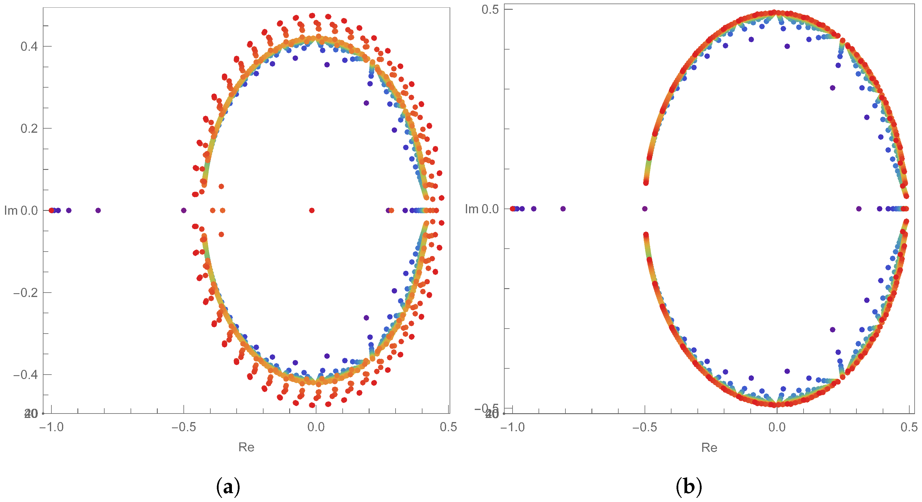
Figure 1 shows the structures of the approximate roots of the q-sigmoid polynomials. The graph in Figure 1a shows the condition of $q=0.1$, while Figure 1b shows the condition of $q=0.0001$. Under the condition of $0<n\le 50$, we can observe Figure 1, which is a figure that appears when viewed from above in 3D. The blue dots are the positions of the approximate roots that appear when the value of n is small, and the red dots are the positions of the approximate roots that appear when $n=50$. Here, as the value of q is smaller, we can assume that most points have a certain circular shape, with the exception of only a few points.

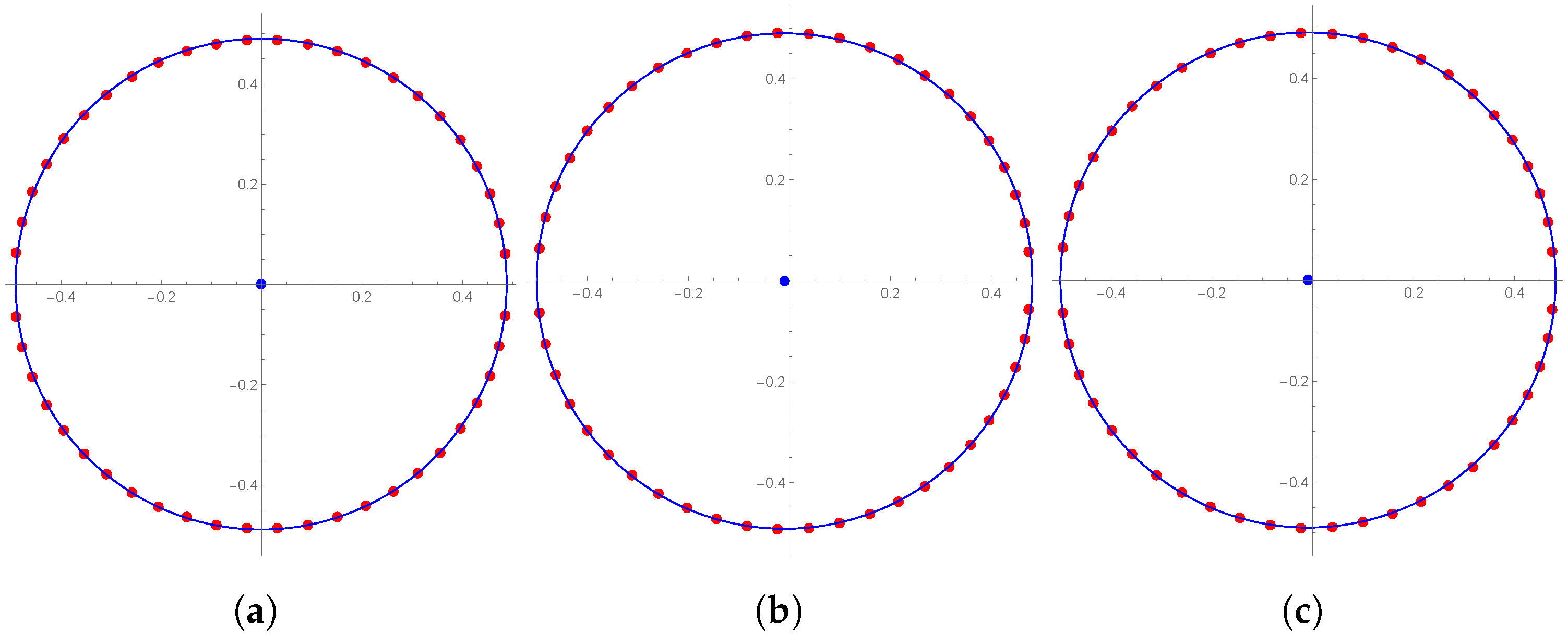
Figure 2 shows the details of the guess made by looking at Figure 1. We fix $n=50$ and change the values of q to $0.01$, $0.001$, and $0.0001$, respectively. Figure 2a show the results with the value of q set to $0.01$, Figure 2b shows the results with $q=0.001$, and Figure 2c shows the results with $q=0.0001$. In Figure 2, the red dots indicate only imaginary roots except for the real roots, and the blue lines indicate the closest circle to the approximate roots. The blue dot represents the center of the approximated circle. Figure 2 shows that the approximated root positions lie on a circle.

Table 1. The center and radius of the approximated circles of ${\mathcal{S}}_{50,q}\left(x\right)$.

	The Center (x, y)	$\mathbf{The}\mathbf{Radius}$	$\mathbf{The}\mathbf{Error}\mathbf{Range}$
$q=0.01$	$(-0.0013679,4.21363\times {10}^{-13})$	$0.489466$	$0.00013278$
$q=0.001$	$(-0.00911017,-8.92717\times {10}^{-12})$	$0.490576$	$0.0000920933$
$q=0.0001$	$(-0.00890715,1.6445\times {10}^{-12})$	$0.490528$	$0.0000711247$

below is the result of accurately calculating Figure 2 using a computer. In Table 1, it can be seen that the center of the approximated circle is slightly shifted to the left when the value of q is smaller. Furthermore, it can be seen that the radius is closer to $0.4905$ when the value of q is smaller. It can be observed in Table 1 that when the value of q is smaller, the error ranges of the approximated circle and the approximate roots are smaller as well; in other words, the positions of the approximate roots are located on the approximated circle. Here, we can make the following assumptions.

Conjecture 11. 

The locations of the approximation roots of q-sigmoid polynomials lie on the approximated circle under the condition in which $n=50$ and $q=0.001$.

In Figure 1, it can be seen that, in addition to the circle, there are red dots, blue dots, etc., on the left side.

Table 2. Approximate real roots of ${\mathcal{S}}_{n,q}\left(x\right)$.

	q	0.01	0.001	0.0001
n
⋮		⋮	⋮	⋮
5		$-0.983547$	$-0.983031$	$-0.98298$
6		$-0.992142$, $0.415504$	$-0.991826$, $0.419697$	$-0.991795$, $0.420109$
7		$-0.99619$	$-0.996003$	$-0.995984$
8		$-0.998137$, $0.433359$	$-0.998028$, $0.437674$	$-0.998017$, $0.438096$
9		$-0.999084$	$-0.999022$	$-0.999015$
10		$-0.999548$, $0.444653$	$-0.999513$, $0.449039$	$-0.99951$, $0.449468$
⋮		⋮	⋮	⋮
19		$-0.999999$	$-0.999999$	$-0.999999$
20		$-1$, $0.46868$	$-1$, $0.473205$	$-1$, $0.473645$
⋮		⋮	⋮	⋮
29		$-1$	$-1$	$-1$
30		$-1$, $0.47715$	$-1$, $0.481719$	$-1$, $0.482163$
⋮		⋮	⋮	⋮
39		$-1$	$-1$	$-1$
40		$-1$, $0.481477$	$-1$, $0.486068$	$-1$, $0.486516$
⋮		⋮	⋮	⋮

shows the real zeros of these approximation roots.

Based on Table 2, we can consider q-sigmoid polynomials by dividing n into even and odd. When n is an even number, it can be assumed that the q-sigmoid polynomials have two real roots regardless of the value of q-number. On the other hand, it can be assumed that the q-sigmoid polynomials will always have one real root regardless of the q-number when n is odd.

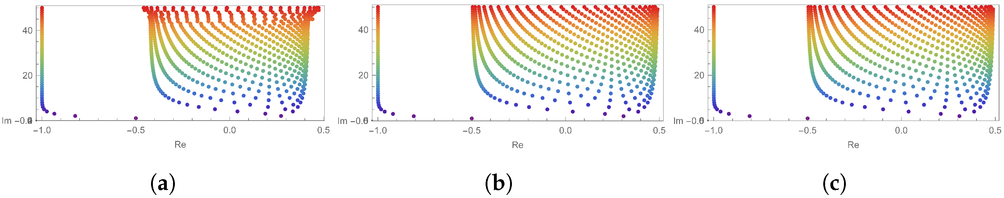
Figure 3 below shows another property of the approximate roots of q-sigmoid polynomials. In Figure 3, we can see that the approximate roots of this polynomial are stacked in two shapes. When $0\le n\le 50$, one shape is a circular shape and the other shape is a straight shape. Because the shape of the circle is confirmed in Figure 2 and Table 1, we consider the straight shape.

Based on Table 2 and Figure 3, we can make the following assumptions.

Conjecture 12. 

(i) Assume that the value of q is very small, while the value od n is even and increasing. Then, the q-sigmoid polynomial has two real approximations.

(ii) Suppose that the value of q is very small, while the value of n is odd and increasing. Then, the q-sigmoid polynomial has only one real approximation.

4. Conclusions

In this paper, we find several types of q-differential equations of higher order and confirm that their solutions become q-sigmoid polynomials. In order to confirm the properties of the q-sigmoid polynomials which are the solutions of these differential equations of higher order, we conducted many different types of experiments based on varying assumptions. To solve these conjectures, it is necessary to study various approaches to special polynomials. In addition, we think that useful results can be obtained by conducting new research based on the defined function in [11].

References

- Jackson, H.F. q-Difference equations. Am. J. Math 1910, 32, 305–314. [Google Scholar] [CrossRef]
- Kac, V.; Cheung, P. Quantum Calculus; Springer: Berlin/Heidelberg, Germany, 2002; ISBN 0-387-95341-8. [Google Scholar]
- Bangerezako, G. An Introduction to q-Difference Equations; University of Burundi: Bujumbura, Burundi, 2008; preprint. [Google Scholar]
- Comtet, L. Advanced Combinatorics; Reidel: Dordrecht, The Netherlands, 1974. [Google Scholar]
- Carmichael, R.D. The general theory of linear q-qifference equations. Am. J. Math. 1912, 34, 147–168. [Google Scholar] [CrossRef]
- Jackson, H.F. On q-functions and a certain difference operator. Trans. R. Soc. Edinb. 1950, 46, 253–281. [Google Scholar] [CrossRef]
- Konvalina, J. A unified interpretation of the binomial coefficients, the Stirling numbers, and the Gaussian coefficients. Amer. Math. Mon. 2000, 107, 10. [Google Scholar] [CrossRef]
- Mason, T.E. On properties of the solution of linear q-difference equations with entire function coefficients. Am. J. Math. 1915, 37, 439–444. [Google Scholar] [CrossRef]
- Rodrigues, P.S.; Wachs-Lopes, G.; Santos, R.M.; Coltri, E.; Giraldi, G.A. A q-extension of sigmoid functions and the application for enhancement of ultrasound images. Entropy 2019, 21, 430. [Google Scholar] [CrossRef] [PubMed] [Green Version]
- Trjitzinsky, W.J. Analytic theory of linear q-difference equations. Acta Math. 1933, 61, 1–38. [Google Scholar] [CrossRef]
- Silindir, B.; Yantir, A. Generalized quantum exponential function and its applications. Filomat 2019, 33, 15. [Google Scholar] [CrossRef]
- Zil, D.G. A First Course in Differential Equations: With Modeling Applications, 9th ed.; Brooks/Cole; Cengage Learning, Inc.: Boston, MA, USA, 2009; ISBN -13: 978-04951082452009. [Google Scholar]
- Han, J.; Wilson, R.S.; Leurgans, S.E. Sigmoidal mixed models for longitudinal data. Stat. Methods Med. Res. 2018, 27, 863–875. [Google Scholar] [CrossRef]
- Ito, Y. Representation of functions by superpositions of a step or sigmoid function and their applications to neural network theory. Neural Netw. 1991, 4, 385–394. [Google Scholar] [CrossRef]
- Kim, M.; Song, Y.; Wang, S.; Xia, Y.; Jiang, X. Secure Logistic Regression Based on Homomorphic Encryption: Design and Evaluation. JMIR Med. Inform. 2018, 6, e19. [Google Scholar] [CrossRef] [PubMed] [Green Version]
- Kang, J.Y. Some relationships between sigmoid polynomials and other polynomials. J. Appl. Pure Math. 2019, 1, 1–2. [Google Scholar]
- Han, J.; Moraga, C. The influence of the sigmoid function parameters on the speed of backpropagation learning. In Proceedings of the International Workshop on Artificial Neural Networks, Malaga-Torremolinos, Spain, 7–9 June 1995. [Google Scholar] [CrossRef]
- Kang, J.Y. Some properties and distribution of the zeros of the q-sigmoid polynomials. Discret. Dyn. Nat. Soc. 2020, 2020, 4169840. [Google Scholar] [CrossRef]
- Kwan, H.K. Simple sigmoid-like activation function suitable for digital hardware implementation. Electron. Lett. 1992, 28, 1379–1380. [Google Scholar] [CrossRef]
- Ryoo, C.S.; Kang, J.Y. Phenomenon of scattering of zeros of the (p,q)-cosine sigmoid polynomials and (p,q)-sine sigmoid polynomials. Fractal Fract. 2021, 5, 245. [Google Scholar] [CrossRef]
- Andrews, G.E.; Askey, R.; Roy, R. Special Functions; Cambridge Press: Cambridge, UK, 1999. [Google Scholar]
- Gi-Sang, C. A note on the Bernoulli and Euler polynomials. Appl. Math. Lett. 2003, 16, 3. [Google Scholar]
- Endre, S.; David, M. An Introduction to Numerical Analysis; Cambridge University Press: Cambridge, UK, 2003; ISBN 0-521-00794-1. [Google Scholar]
- Ryoo, C.S. Some identities involving the generalized polynomials of derangements arising from differential equation. J. Appl. Math. Inform. 2020, 38, 159–173. [Google Scholar]
Figure 1.
Positions of the approximate roots of with : (a) , (b) .
Figure 2.
Approximate roots and approximated circles of : (a) , (b) , (c) .
Figure 3.
Approximate roots of with : (a) , (b) , (c) .