Article

Improved G-Optimal Designs for Small Exact Response Surface Scenarios: Fast and Efficient Generation via Particle Swarm Optimization

by
Stephen J. Walsh
1,* and
John J. Borkowski
2
1
Department of Mathematics and Statistics, Utah State University, Logan, UT 84322, USA
2
Department of Mathematical Sciences, Montana State University, Bozeman, MT 59717, USA
*
Author to whom correspondence should be addressed.
Mathematics 2022, 10(22), 4245; https://doi.org/10.3390/math10224245
Submission received: 10 September 2022 / Revised: 30 October 2022 / Accepted: 11 November 2022 / Published: 13 November 2022
(This article belongs to the Special Issue Optimal Experimental Design and Statistical Modeling)

Abstract

:
G-optimal designs are those which minimize the worst-case prediction variance. Thus, such designs are of interest if prediction is a primary component of the post-experiment analysis and decision making. G-optimal designs have not attained widespread use in practical applications, in part, because they are difficult to compute. In this paper, we review the last two decades of algorithm development for generating exact G-optimal designs. To date, Particle Swarm Optimization (PSO) has not been applied to construct exact G-optimal designs for small response surface scenarios commonly encountered in industrial settings. We were able to produce improved G-optimal designs for the second-order model and several sample sizes under experiments with K = 1 , 2 , 3 , 4 , and 5 design factors using an adaptation of PSO. Thereby, we publish updated knowledge on the best-known exact G-optimal designs. We compare computing cost/time and algorithm efficacy to all previous published results including those generated by the current state-of-the-art (SOA) algorithm, the G ( I λ ) -coordinate exchange. PSO is hereby demonstrated to produce better designs than the SOA at commensurate cost. In all, the results of this paper suggest PSO should be adopted by more practitioners as a tool for generating exact optimal designs.

1. Introduction

In 1918 Kirstine Smith published guidance for how the residual error variance informs designing an experiment where the ensuing data are used to fit a polynomial model linear in the parameters [1]. This paper’s contribution provided what we now refer to as G-optimal designs for a K = 1 factor experiment supporting a first up to sixth-degree polynomial. Atkinson and Bailey [2] note that Smith’s contribution is considered the seminal optimal design paper and was 30 years ahead of its time. Optimal design did not receive a rigorous theoretical development until the late 1950s with primary contributions from Kiefer and Wolfowitz [3,4,5]. These contributions focus on the theory of continuous optimal designs (often called approximate or asymptotic designs), that is, designs viewed as a probability measure. The core theory of continuous designs is mathematical in nature and includes the foundational General Equivalence Theorem which provides a way to verify the optimality of a candidate design.
Exact optimal designs, in contrast, are those that are optimal for an integer valued number of experimental runs N. Thus, an implemented experiment utilizes an exact design. Exact designs have no theory analogous to that of continuous designs with which to verify the optimality of a candidate design. Therefore, much of the research into generating exact designs has focused on algorithm development. Early algorithms for generating exact optimal designs date back to the 1970s and include the point-exchange and DETMAX [6,7]. Such algorithms discretize the design space via a candidate set (usually a high order factorial design). The most popular contemporary algorithm for generating exact optimal designs appears to be the Coordinate-Exchange (CEXCH) of Meyer and Nachtsheim [8] which, in contrast to the point exchange, honors a continuous design space and allows any point in the design region to be a component of the experiment.
CEXCH’s success and popularity notwithstanding, it is not without drawbacks. CEXCH is well-recognized to be a local optimizer and so several authors recommend applying CEXCH thousands of times in order to ensure the generation of a highly efficient design [9]. Because CEXCH starts with a single random candidate design followed by a local optimization, it is unlikely, especially in higher dimensional problems, that CEXCH will find the globally optimal design. This fact has motivated several authors to explore the class of meta-heuristic evolutionary algorithms for optimal design generation. Meta-heuristics include the Genetic Algorithm (GA), Simulated Annealing, and Particle Swarm Optimization (PSO) among others. See, for example applications in optimal design, [10,11,12,13,14,15,16,17,18,19]. Simulated Annealing appears to be widely popular, but has not been applied to the G-optimal design problem to date [19]. Meta-heuristics offer attractive solutions to the optimal design problem for two primary reasons. First, they make little to no assumptions regarding the nature of the objective (optimality criterion). Furthermore, second, as opposed to CEXCH, they attempt to search the space of candidate design matrices globally and are robust to entrapment in local optima thereby giving them a significant advantage over CEXCH to generate a highly efficient design in a single run. This benefit, however, often comes at a significant increase to computing cost vs. the CEXCH [11].
Among the meta-heuristics, PSO is a relative newcomer to optimal design, and most applications have been toward generating continuous designs or space-filling designs [13,14,15,16,17,18,20,21]. A comprehensive review of the last decade of research literature on PSO adaptations to experimental design is provided by Chen, Chen, and Wong (2022) [22]. These authors highlight recent applications of PSO for generating continuous optimal designs, minimax/maximin optimal designs (e.g., the G-optimal design problem, or optimal design for non-linear models), and exact optimal designs. Of the sixteen papers on PSO for experimental design discussed in Chen, Chen, and Wong (2022), only one works with exact designs and this is not the primary focus of the paper. Therefore, the literature is lacking demonstration of PSOs efficacy and efficiency to generating exact optimal designs, and specifically those to response surface scenarios commonly encountered by industrial practitioners. More recently, Walsh and Borkowski (2022) [23] present data from a detailed case-study on the efficiency and efficacy of PSO to generating exact optimal designs for 21 small exact response surface scenarios. In short PSO, and specific a version of PSO which uses a random local communication topology, is shown to generate highly efficient designs (efficiency >95%) with large probability (near 1), and an appreciably large probability of finding the global optimal designs for the D- and I-criteria in these scenarios. Therefore, we expect PSO to perform well when applied to the G-optimal exact design generation problem.
In light of the existing literature we designed a detailed study and applied PSO to generate exact G-optimal designs and offer the following contributions to the state-of-knowledge:
1.
A brief literature survey of the last 20 years of algorithm development and approaches for generating exact G-optimal designs in small exact response surface scenarios.
2.
Application of the PSO version with local communication topology, as described in Walsh and Borkowski (2022) to generating exact G-optimal designs for 29 design scenarios for K = 1 , 2 , 3 , 4 , 5 experimental factors and a range of N (experiment sizes) [23].
3.
For most of the 29 design scenarios, PSO was able to find a better G-optimal design than those currently known, and we provide a detailed catalogue of these new designs in the Supplementary Material.
4.
Quantitative benchmarking of PSOs efficiency and efficacy to accomplish this task and performance comparison to state-of-practice and SOA CEXCH type algorithms as illustrated in Rodriquez et al. (2010) and Hernandez and Nachtsheim (2018) [11,24].
The remainder of this paper is organized as follows. In Section 2, we provide notation and define the exact G-optimal design generation problem. In Section 3, we present a literature review of recent research on generating exact G-optimal designs. In Section 4, develop an extension of PSO for generating G-optimal designs. In Section 5, we present the structure of our study for adapting PSO to generate exact G-optimal designs. In Section 6, we present the results where we compare G-PSO generated designs to those provided by [10,11,24]. In Section 7, we provide discussion, conclusions, and future research directions.

2. G -Optimal Design for Small Exact Response Surface Scenarios

2.1. Small Exact Response Surface Designs

As is standard at the optimization step of response surface methodology (RSM), we will be working with the second-order linear model under standard assumptions. Let N represent the number of design points and K represent the number of experimental factors [25]. A design point is an x : 1 × K row-vector. In RSM all design factors are scaled to range [−1,1] and so the design space is the X = [ 1 , 1 ] K hypercube [9,25]. Let X : N × K represent the design matrix, while X denotes the space of candidate design points x , a design matrix X is a collection of N such design points. Thus, the space of all candidate designs is an N K -dimensional hypercube and is denoted:
X j = 1 N X = j = 1 N [ 1 , 1 ] K = [ 1 , 1 ] N K = X N .
The second-order linear model which has p = ( K + 2 2 ) linear coefficient parameters. In scalar form the model is written
y = β 0 + i = 1 K β i x i + i = 1 K 1 j = i + 1 K β i j x i x j + i = 1 K β i i x i 2 + ϵ .
Let F ( X ) : N × p represent the model matrix with rows given by the expansion vector f ( x i ) = ( 1 x i 1 x i 2 x i 1 x i 2 x i ( K 1 ) x i K x i 1 2 x i K 2 ) . Note that we will abbreviate the model matrix F , but it is always a function of the design matrix X . The model can be written in vector-matrix form as y = F β + ϵ where we impose the standard ordinary least squares assumptions ϵ N N ( 0 , σ 2 I N ) where N N denotes the N-dimensional multivariate normal distribution. The ordinary least squares estimator of β is β ^ = ( F F ) 1 F y which has variance Var ( β ^ ) = σ 2 ( F F ) 1 . The total information matrix for β , specifically M ( X ) = F F , plays an important role in optimal design of experiments—all optimal design objective functions are functions of this matrix [9].
The practitioner must choose a design from X N to implement the experiment in practice. An optimality criterion is used to define which candidate designs X X N are ‘good’ designs. An optimization algorithm is required to search X N to find the ‘best’, or optimal, design. Thus, an exact optimal design problem is defined by three components:
1.
The number of design points N that can be afforded in the experiment.
2.
The structure of the model one wishes to fit (here the second-order model).
3.
A criterion which defines an optimal design. This is a function of M ( X ) .
In the next subsection we define the G-criterion and G-optimal design.

2.2. G-Optimal Design

A G-optimal design is that design which minimizes the maximum (i.e., worst case) prediction variance over X . The the variance of the mean predicted value is
Var ( y ^ ( x ) ) = σ 2 f ( x ) ( F F ) 1 f ( x )
for any point of prediction x X . The scaled prediction variance (SPV) removes the scale parameter σ 2 and re-scales to N by multiplying by the factor N / σ 2 . Thus, SPV is defined as (for a candidate design X )
SPV ( x | X ) : = N f ( x ) ( F F ) 1 f ( x ) .
The G-score of a candidate design X is defined as the maximum scaled prediction variance over all points of prediction x X
G ( X ) : = max x X SPV ( x | X ) .
Equation (3), thus, shows that for a fixed candidate design X , scoring the candidate on the G scale is itself an optimization problem. The G-optimal design X * is that design which minimizes, over all designs X X N , the maximum scaled prediction variance, namely
X * : = argmin X X N G ( X ) = argmin X X N max x X SPV ( x | X ) .
Equation (4) shows that finding the G-optimal design is a minimax problem. This optimization has proved notoriously difficult to solve because neither of the optimizations required to compute X * are convex in large part due to the expansion of the design matrix into model matrix F [10,11,24].
The scale of G for an arbitrary design has known bounds. The General Equivalence Theorem of [3] demonstrates that the lower bound on G ( X ) is
G ( X ) = max x X SPV ( x ) p .
That is, the smallest that the maximum scaled prediction variance of candidate design X may be is p, the number of parameters. This apparently gives a way to verify if a proposed exact G-optimal design is globally optimal, however, not all design scenarios have globally G-optimal designs that will achieve this lower bound. Further, if design X * is globally G-optimal and achieves the result in Equation 5, then for this design SPV ( x | X ) = p at all diagonals of the hat matrix F ( F F ) 1 F and SPV ( x | X ) p at all other points of prediction x X [25]. It is customary to exploit this fact and score candidate designs on the G-efficiency scale,
G eff ( X ) = 100 p G ( X ) ,
in order to gauge the quality of a candidate design X (larger G eff on this scale implies a better design). Last, the relative efficiency of two candidate designs may be computed as
G releff ( X 1 , X 2 ) = 100 G eff ( X 1 ) G eff ( X 2 ) .
In the next section, we provide a review of the most literature for generating G -optimal designs for small exact response surface models.

3. Literature Review: Algorithm Development and Current Best-Known Exact G -Optimal Designs

The exact G -optimal design generation problem is recognized as the notoriously difficult mini-max problem expressed in Equation 4. It was not until recent decades that modern computing resources were cheap enough to enable the application of well-suited meta-heuristic optimization approaches to this problem. Borkowski [10] provided one of the earliest applications of Genetic Algorithms (GAs) for generating exact optimal designs over the hypercube supporting a second-order response surface model in K = 1 , 2 , 3 design factors and for experiment sizes N = 3 , 4 , 5 , 6 , 7 , 8 , 9 , N = 6 , 7 , 8 , 9 , 10 , 11 , 12 , and N = 10 , 11 , 12 , 13 , 14 , 15 , 16 , respectively. Borkowski [10] adapted a GA to generate G -, D -, I -, and A -optimal designs and published a proposed catalog of exact optimal designs for each criterion. The results provided in [10] have become a ‘ground truth’ standard data set against which to compare results of newly developed algorithms to solve this problem. Until this point, the exact G -optimal designs of Borkowski (2003) have remained the best-known designs for these scenarios [10] and were subsequently reproduced by [24] via an augmented application of the coordinate exchange, and used as a benchmark dataset for new algorithms proposed by authors [11,26].
Next, [24] adapted the coordinate exchange (CEXCH) algorithm of [8] in conjunction with Brent’s minimization algorithm (used to score a candidate design on the G -scale) to generate exact G -optimal designs. These authors covered all scenarios or K = 2 , 3 design factors as in Borkowski (2003) and were able to reproduce these designs with their new algorithm. These authors extend [10] and propose candidate exact G -optimal designs for K = 4 , N = 15 , 20 , 24 and K = 5 , N = 21 , 26 , 30 . Note that, to this point, K = 4 , 5 G -optimal designs had not been explored because of prohibitive computational cost. A third contribution of this work was a detailed comparison of the resulting G -CEXCH generated exact G -optimal design’s properties (via fraction of design space plots) with corresponding D - and I -optimal designs. The authors found that, for scenarios where post hoc prediction was the primary objective, the I -optimal designs exhibited smaller prediction variance than the corresponding G -optimal designs over large percentages of the design space (even though the G -optimal design has lower maximum prediction variance). This observation motivated the authors to recommend that the additional computing cost required for G -optimal designs may not be worth the effort and I -optimal designs might be preferred for many practical experimental scenarios. The G - vs. I -optimal design question is the subject of ongoing research in the broader literature [27].
Saleh and Pan (2015) recognized the lack of algorithm development on the G -optimal design problem and provide a hybridized point and coordinate exchange algorithm which utilizes clustering to explore the characteristics of SPV over the design space [26]. Their algorithm is termed cCEA and they apply it to linear model and generalized linear model scenarios. cCEA proceeds by first by generating a large set of candidate design points x to provide a covering of X . These points are fed into a clustering algorithm to produce families of design points over X based on SPV. For a candidate design, these clusters are scored on the SPV scale. A point exchange algorithm is applied to the candidate and each cluster is rescored on SPV. The algorithm proceeds until no further reductions in maximum SPV are found. In the second step, standard CEXCH locally adjusts the candidate in order to find a design that further reduces the SPV. In short this algorithm attempts to get a design close to G -optimal quickly via the clustering and point exchange, and then refines this design locally using the standard coordinate exchange. With cCEA, these authors were able to nearly reproduce designs with scores equivalent to [10,24].
The most recent publication on generating exact G -optimal designs is offered by [11]. The primary focus of this paper is the computational cost associated with generating G -optimal designs. These authors noticed a correspondence between continuous I λ -optimal designs and G -optimal designs. They propose a new algorithm that exploits the structural relationship between these two types of designs which first generates a continuous I λ -optimal design as a starting point for the exact G -optimal design search. Then they apply the CEXCH algorithm to locally improve the candidate G -optimal design. We will refer to their algorithm as G ( I λ ) -CEXCH. These authors are the first to completely run G ( I λ ) -CEXCH and rerun the searches via GA by Borkowski (2003) in Matlab, and CEXCH by [24] in JMP (they also reported the architecture of their PC) in order to compare computing efficiency of their proposed algorithm to the others. They implemented 200 runs of each algorithm for each design scenario discussed in [10] and also ran two new scenarios: K = 4 , N = 17 and K = 5 , N = 23 with only G ( I λ ) -CEXCH (they indicated that CEXCH would have taken 25 and 166 days, respectively, to complete the task, and so this algorithm was not run on these scenarios). These authors found that the GA was able to find the most efficient G -optimal designs in repeated runs, but that CEXCH and G ( I λ ) -CEXCH produced designs with high relative efficiency vs. GA generated designs with relative-efficiencies of 90% or greater at a fraction of the cost [11]. Thus, the GA achieves this superiority at high computational cost exhibiting 2-orders of magnitude increase in the number of objective function evaluations as compared to the G ( I λ ) -CEXCH. G ( I λ ) -CEXCH was demonstrated to produce designs with high G -efficiency as well as standard CEXCH but with computing times at a fraction of CEXCH for the higher dimensional searches. Thus, they propose that G ( I λ ) -CEXCH is a good choice for generating exact G -optimal designs as it is demonstrated to produce designs with high relative efficiency to GA generated designs and does this more efficiently than existing algorithms.
Last, in Table 1 we present a summary of exact G -optimal design scenarios that authors have addressed in previous algorithm development and research, and that we will study further using PSO in this paper.

Evaluating the G -Score for Candidate Design X

Any algorithm needs to address both optimizations expressed in Equation 4, or more specifically, given a candidate design X , one must score it on the G -scale via Equation 3. There are two approaches to doing this implemented in the algorithms discussed in the previous section.
First, authors [10,11] exploit the symmetry of the SPV-surface for a G -optimal design and recommend using a 5 K point grid over X with each factor containing x j { 1 , 0.5 , 0 , 0.5 , 1 } for j = 1 , , K grid-points. The full grid defined as G X = { 1 , 0.5 , 0 , 0.5 , 1 } K [11]. Once one has a candidate design, the SPV is evaluated on G X and the maximum value is taken as an approximation of the G -score for the candidate design, while this approach computes an approximate G -score for a candidate design X both authors have noted that, due to the symmetry of the quadratic G -surface for G -optimal designs, the approximation is quite adequate giving small errors and supports finding highly G -optimal designs.
Authors [24,26] use a different mechanism to compute G for a candidate design X. Ref. [26] use the clustering and point exchange phase of their algorithm. In [24], once a candidate is available (e.g., after every coordinate exchange) they employ Brent’s minimization algorithm to search for the maximum prediction variance for the candidate design over X.
Regarding the choice of method for scoring a candidate design on the G -scale in this paper: we implemented the 5 K grid approach recommended by [10,11] for several reasons. Similar to authors [10,11] we find that this approach yields G -optimal design candidates with small error on the G -eff scale. Further, we ran a pilot study using a nested PSO approach [20] but similar to [24] we observed that if the inner PSO search to score a candidate design on the G -eff scale mis-scored the candidate design, this error propagated through the outer PSO search and reduced the success of finding the globally optimal design.
In the next section we describe the PSO algorithm and provide an extension of PSO to generate G -optimal designs used to produce the results presented in this paper.

4. Particle Swarm Optimization for Generating Optimal Designs

PSO is a wildly popular meta-heuristic optimization approach which has been widely applied to great success across engineering applications and applied science problems. To date, the seminal paper by [28] has 73,647 citations (queried in Google Scholar on 8 August 2022). PSO has been demonstrated to perform very well for high-dimensional optimization of multimodal objective functions, see for example, [28,29,30,31,32,33,34,35,36,37,37]. PSOs strengths include:
1.
few-to-no assumptions about the properties of the objective function f to be optimized,
2.
PSO is demonstrated to be robust to entrapment in local optima, and thereby is a good match to the exact optimal design generation problem,
3.
simplicity—the core function of the algorithm can be explained via two simple update equations, and
4.
in contrast to other meta-heuristics where studying a range of tuning parameters can yield more efficient searches for specific problems, PSO only has three tuning parameters and these have been studied extensively, both theoretically and empirically, with optimal values demonstrated for searches (such as ours) that reside in the common Cartesian product space with the typical Euclidean geometry, see [34,38,39,40] among others.
PSOs widespread application notwithstanding, we observe relatively few applications in Statistics and specifically Optimal Design. The first such application in 2013 by Chen et al. discussed PSO-generated latin-hypercube designs [14]. Application of PSO to generating space-filling designs is addressed by [13,17]. PSO for generating optimal designs for non-linear models is illustrated in [15,16,20]. PSO-generation of Bayesian continuous designs is discussed in [21] and PSO for constructing continuous optimal designs for mixture experiments is provided in [18]. More recently [23] provided a benchmarking study on PSO for generating small-exact response surface designs under the D - and I -criterion. These authors show that a version of PSO which utilizes a local communication topology is superior to standard PSO which uses global communication topology in the sense that it greatly increases the probability that PSO will find the globally optimal design in a single run of the algorithm [23]. We expect these results to be similarly realized for the G -optimality searches as conducted in this paper.
We present the full PSO algorithm, extended to optimize functions that take matrix inputs, in Algorithm 1. The primary difference of our exposition of PSO vs. the standard PSO literature is that our version in Algorithm 1 is a clear formulation that works on functions that take matrix inputs as opposed to vector inputs. A brief dictionary of all quantities is
  • S := number of candidate designs (i.e., particles) in the swarm,
  • X i : N × K := candidate design i ,
  • P best , i := the best design found by particle i ,
  • L best , i := the best design found by the particles in particle is communication neighborhood,
  • G best := the best best design found by the swarm; this is the proposed optimal design,
  • U K ( l b , u b ) = K -dimensional multivariate uniform distribution with lower and upper bound vectors l b and u b , respectively,
  • U = { u i j } i = 1 , j = 1 N , K := random matrix with elements u i j i . i . d U ( 0 , 1 ) ,
  • ⊙:= Hadamard product (elementwise multiplication).
Algorithm 1: PSO for Generating Exact Optimal Designs on the Hypercube
1:
Input: Objective function f , number of particles S , search space bounds l b = 1 K and u b = 1 K
2:
// Randomly draw S candidate designs X i and initialize
3:
for each i = 1 , , S do
4:
   x i j U K ( l b , u b ) for j = 1 , , N giving candidate design X i with rows x i j
5:
   v i j U K l b x i j 2 , u b x i j 2 for j = 1 , , N giving velocity matrix V i with rows v i j
6:
   { v i j k min { v i j k , v k max } } for j = 1 , , N  // limit stepsize
7:
   N i genNeighbors ( X i ) // generate communication neighborhood for particle i
8:
   P best , i X i  //set initial personal best position
9:
endfor  
10:
G best argmin X i { X 1 , X 2 , , X S } f ( X i ) // current best design among swarm  
11:
L best , i argmin X i N i f ( X i ) for i = 1 , , S  // current best design in local neighborhoods  
12:
// swarm search loop
13:
while stopping criteria not met do (this is iteration over t )
14:
  if  G best ( t ) = G best ( t 1 )
15:
    // if the solution does not improve, reform the local communication networks
16:
     N i genNeighbors ( X i )
17:
  endif
18:
  for each i = 1 , , S  do // Update velocities and positions
19:
     V i ω V i + c 1 U P best , i X i + c 2 U L best , i X i
20:
     { v ijk min { v i j k , v k max } } for j = 1 , , N
21:
     X i X i + V i
22:
     X i confine ( X i )  // keep candidates in searchspace
23:
    if  f ( X i ) < f ( P best , i ) // update knowledge about best known design to time t
24:
       P best , i X i
25:
      if  f ( P best , i ) < f ( G best )
26:
         G best P best , i
27:
      endif
28:
    endif
29:
  endfor
30:
  for each i = 1 , , S  do // with personal best’s update, can update local best
31:
    if  f ( P best , i ) < f ( L best , i )
32:
       L best , i P best , i  // update best known design in local neighborhoods
33:
    endif
34:
  endfor
35:
endwhile  
36:
Output: Particle swarm solution—the best optimal design found G best
We briefly identify core components of the algorithm as follows. Lines 4 and 5 show how the S initial candidate designs are randomly constructed based on a multivariate uniform distribution. We employ Standard Particle Swarm 2007 which utilizes a local communication topology [30]. Therefore line 7 indicates a sub-routine genNeighbors which randomly initializes particle matrix is communication neighborhood. This local communication topology has been illustrated to increasing the chance that the swarm finds the global optimal design. The core velocity update equation is stated in line 19 which shows that particle is step size and direction is a weighting of the typical inertia, cognitive, and social components. We implement the optimal recommended values for the weighting parameters
ω = 1 log ( 2 ) , c 1 = c 2 = 1 2 + log ( 2 ) .
These values have been illustrated theoretically and empirically to provide an excellent balance between exploration and exploitation while guaranteeing that the swarm eventually converges to a consensus solution [30,34,41].

5. Study Structure: Experimental Design and PSO Run Parameters

We implemented Algorithm 1 in the Julia language [42]. Our machine is an Intel i7-6700K which has 4 cores and 8 compute threads running at 4.0GHz. Thus, we could send multiple runs of PSO to 7 of the cores at the same time. We ran G -PSO n run = 140 times for all design scenarios (and searches for the optimal design that supports the second-order model) covered by [10]. These scenarios cover K = 1 , 2 , 3 design factors with experiment sizes N = 3 , 4 , 5 , 6 , 7 , 8 , 9 , N = 6 , 7 , 8 , 9 , 10 , 11 , 12 , and N = 10 , 11 , 12 , 13 , 14 , 15 , 16 , respectively. Both [10,11] ran the GA for these scenarios, but, they did not find the same exact G -optimal designs (in part related to the stopping criterion implemented by [11]). Regarding G -optimality, [10] found the current best-known G -optimal designs (to this point). Hernandez and Nachtsheim (2018) [11] found highly G -efficient designs relative to those of [10], but used their GA generated designs to compare their results from the other two algorithms in their study. We also ran G -PSO n run = 210 times for the additional scenarios in [24]. These scenarios cover K = 4 , 5 with experiment sizes N = 15 , 20 , 24 and N = 21 , 26 , 30 , respectively. Last, we ran G -PSO n run = 210 for the additional scenarios in [11], specifically K = 4 , N = 17 and K = 5 , N = 23 . Our stopping criteria for all PSO runs was either a non-zero change in the objective equal to the square root of machine epsilon (about 10 × 10−8, or if the objective score stagnated for 100 iterations, we terminated the run and started a new run [23].
In total we have covered all published exact G -optimal designs for 29 design scenarios requiring 4620 independent runs of PSO. In the next section we compare G -PSO results to those of [10,11,24].
Hernandez and Nachtsheim (2018) [11] is the only reference that reported computing cost among our references, and they offer two measures: (1) number of function evaluations over all runs for each design scenario and (2) computing time wall-clock for the set of searches for each algorithm and design scenario and so a way to check the efficiency of G -PSO relative to the state-of-the-art. We will compare the efficiency of PSO to the other algorithms by reporting number of function evaluations during the runs of PSO. This measure is, of course, senstive to the number of particles and the stopping criterion. We ran all PSO searches with S = 150 particles.

6. Results

6.1. The K = 1 , 2 , 3 Design Scenarios

The proposed G -optimal designs generated by the GA implemented by [10] were reproduced by G -CEXCH in [24] and heretofore have remained the best known exact G -optimal designs for the second-order model and each of the K = 1 , 2 , 3 design scenarios. We provide a comparison of the n run = 140 PSO search results (for each scenario) to the G -GA designs of [10] in Figure 1. The data presented in this graphic are efficiencies of the G -PSO designs relative to the single best found G -GA designs. Therefore, scores over 100 indicate that the PSO generated design is an improvement over the GA generated design. For the K = 1 scenarios, which are low-dimensional optimization from 3 to 9 dimensions, the graphic illustrates that all PSO runs are finding designs with equivalent G -score relative to the GA designs. In the second panel the results for the K = 2 designs now shows a distribution in the G -releff score, but, for each scenario, the PSO produced designs with 90% relative efficiency or higher for every single run. Further, PSO found a better G -optimal design for design sizes N = 9 , 10 , 11 , 12 . The last panel of the graphic indicates that, for K = 3 factors and all experiment sizes N , PSO has identified an improved G -optimal design than those currently known, and the improvements are non-negligible, with increases ranging from 2 to 8% efficiency.
Hernandez and Nachtsheim [11] provides a comparison of G ( I λ ) -CEXCH, G -CEXCH and G -GA and their relative ability to generate designs with the highest/best G -optimality. We note that, in their data, [11] did not compare their results to the G -GA designs as published by [10], rather, they re-ran the GA algorithm n run = 200 times in order to compare relative costs of the algorithm. Thus, the G -GA optimal designs in [11] are equal to or less efficient than those of [10]. Nonetheless, we can use their data to compare all algorithms vs. the GA designs of [10] (which are the best known to date). Table 2 reports the efficiencies of the optimal design relative to the GA design found by [10] for each scenario and algorithm. In all cases, it can be seen that PSO finds the best design vs. all other algorithms.
Regarding computing cost, run time wall-clock for the entire set 140 × 21 = 2940 of PSO searches over K = 1 , 2 , 3 factors and the N aforementioned was approximately 30 min (recall we are using Julia as well as running independent PSO searches in parallel on separate CPU cores). Hernandez and Nachtsheim [11] provides algorithm cost in the form of number of function evaluations over n run = 200 runs of G ( I λ ) -CEXCH, G -CEXCH and G -GA. Table 3 contains comparison of the [11] cost data to the cost of running G -PSO over our n run = 140 runs. We provide a comparison of G -PSO cost on [11]’s n run = 200 run scale by estimating the expected number of function evaluations and a 95% confidence interval via Poisson statistics. Table 3 shows that GA is the most expensive algorithm, and often via 2 orders of magnitude for the higher-dimensional problems. G ( I λ ) -CEXCH is slightly more costly than G -CEXCH for the lower dimensional problems, but is cheaper for the higher dimensional problems (often by an order of magnitude). Last, the 95% confidence interval on the expected number of function evaluations in 200 PSO searches indicates that, in all cases, G -PSO has approximately the same cost as the new G ( I λ ) -CEXCH (with some scenarios being slightly higher, but many scenarios being slightly lower cost than G ( I λ ) -CEXCH).
These results illustrate that G -PSO is approximately the same cost as the state-of-the-art algorithm G ( I λ ) -CEXCH for generating G -optimal designs, while PSO generates highly optimal designs more efficiently, as it is demonstrated here to produce the current best-known exact G -optimal designs for these scenarios.

6.2. The K = 4 , 5 Design Scenarios

Due to the computational cost, this number of experimental factors is the highest that the design community has gone to date. Searching for G -optimal designs for more factors will take a considerable time/computing investment. Note, however, that K does not define the dimension of the optimization search: the dimension is N K so the largest problem we study here is K = 5 , N = 30 which is an optimization search in a 150 dimensional search space.
Table 4 contains the G -efficiencies of the best G ( I λ ) -CEXCH, G -CEXCH, and G -PSO generated design, as well as the relative efficiency of the G -PSO design to the indicated CEXCH algorithm. In all cases PSO is found to generate better G -optimal designs, and in some cases with a significant improvement. We present distributions of the G -releff scores of the PSO designs to the corresponding CEXCH generated designs in Figure 2. In all cases it can be seen that PSO found an equivalent or better G -optimal design (evidenced by relative efficiencies over 100). We note that each of the CEXCH algorithms was run n run = 200 times in the work of [11] and the PSO searches were run n run = 210 times (a number evenly distributed on 7 computer cores). The graphic further illustrates PSO’s ability to seek highly optimal designs each run, evidenced by the distributions of G -releff being tightly packed at or over 100% relative efficiency. For many scenarios, there is apparently a high probability that PSO would generate a design with 95% efficiency or better in a single run.
Regarding the significant improvements in designs, first for the K = 4 ,   N = 15 case PSO provided a design with 145% relative efficiency to the best-known design. Second, for the K = 4 ,   N = 20 scenario, PSO produced a design with 123% improved efficiency. Furthermore, last, for the K = 5 ,   N = 21 scenario, PSO found a design with 177% relative efficiency. We contacted the authors of [24] to investigate these large discrepancies. For the K = 4 ,   N = 15 and K = 5 ,   N = 21 scenarios, it was confirmed that the designs published by [24] were mis-scored on the G -scale (personal email correspondence with Dr. Bradley Jones, 20 June 2020). Given that [24] employs a separate optimization search to score each candidate design on the G -scale, these results illustrate the consequences of failing to find the maximum prediction variance for a candidate design, and, to our opinion, support the approach of using the 5 K grid G X to score candidate designs.
The information for a proper time comparison for generating designs with K = 4 ,   5 factors via PSO vs. the other approaches does not exist due to algorithms being run on different machines and computing languages. Nonetheless, for information we report what data do exist for computing times on the K = 4 ,   N = 17 and K = 5 ,   N = 23 design scenarios. Hernandez and Nachtsheim [11] report that they were able to run G ( I λ ) -CEXCH n run = 200 times on the K = 4 ,   N = 17 in 20.13 h on their computing platform (approx 6.0m for each run). They were not able to run G -CEXCH as they estimated that 200 runs would have taken 25 days on their machine. Our approach (PSO, Julia, n run = 210 parallel PSO runs [30 runs per 7 cores]) took about 3 h which translates into approximately 6 m per each individual run. Hernandez and Nachtsheim [11] report that they were able to run G ( I λ ) -CEXCH n run = 200 times on the K = 5 ,   N = 23 in 25.07 h on their computing platform (approx 7.5m for each run). They were not able to run G -CEXCH as they estimated that 200 runs would have taken 166 days on their machine. Our approach (PSO, Julia, n run = 210 parallel PSO runs [30 runs per 7 cores]) took about 20h which translates into approximately 40 m per each individual run. These results imply that PSO has more difficulty scaling to higher dimension. The reason why PSO took approximately 6 times longer for the K = 5 scenario than for the K = 4 scenario is that the respective 5 K grids used to score each candidate design during the search have 5 5 = 3125 and 5 4 = 625 points, respectively, and each particle (i.e., each candidate design) must have the G -score evaluated at each of these grid points, at each iteration of the algorithm. Nonetheless, we believe this time increase to be of little hindrance to scaling PSO to efficient searches for higher dimensional designs due to the use of Julia and parallel computing, and the additional cost is easily mitigated via CPUs with more computer cores.

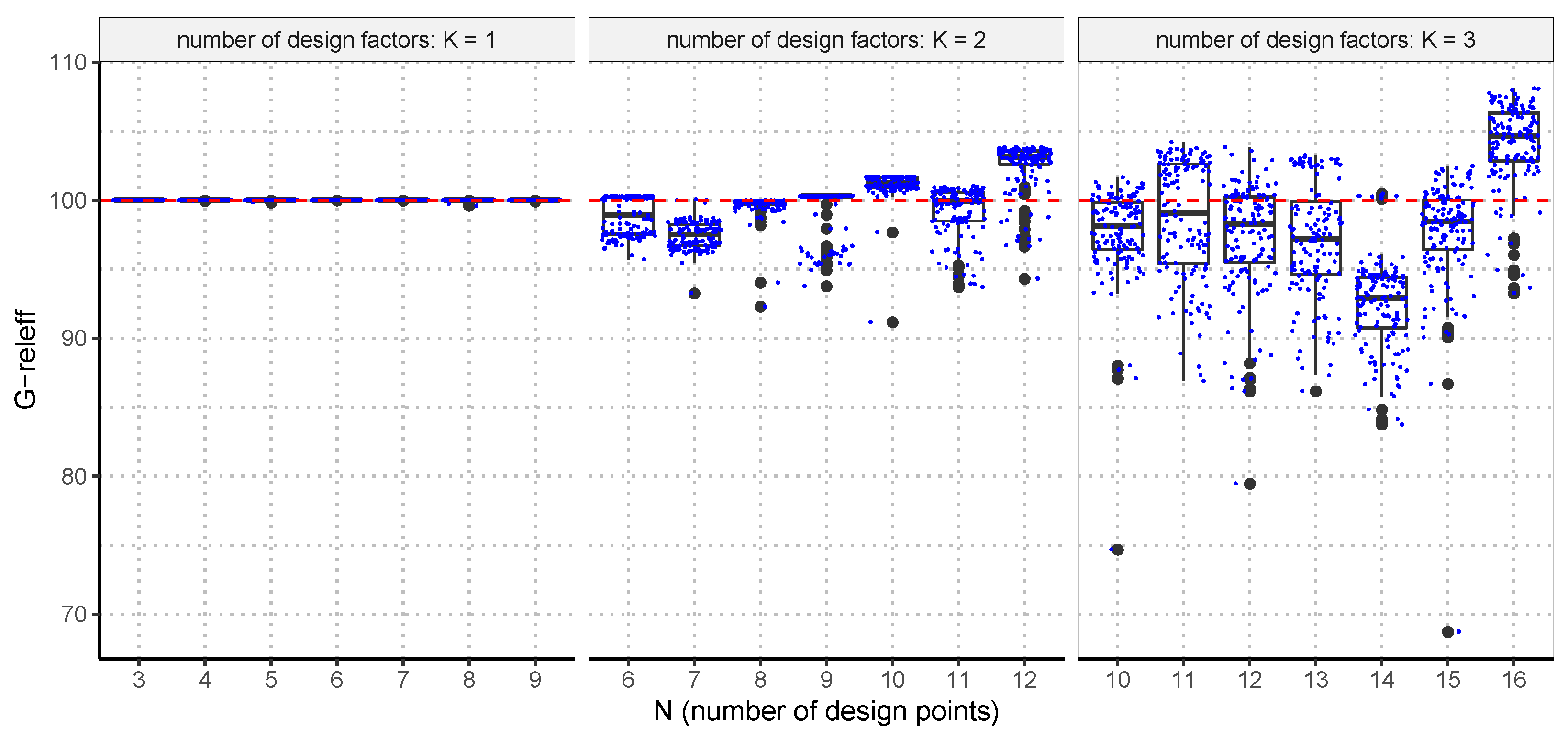
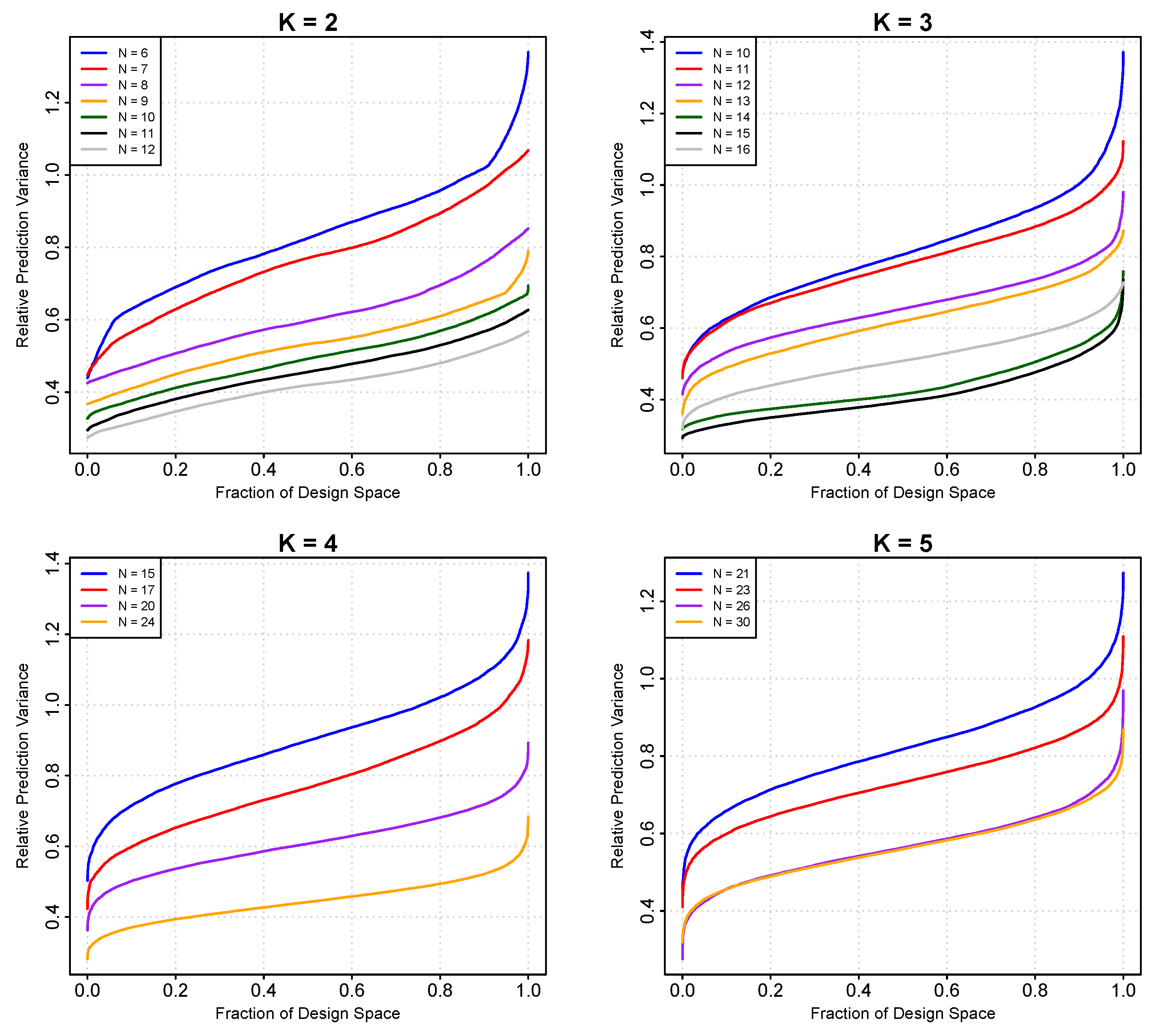
6.3. Prediction Variance Properties of the New G -Efficient Designs

We publish fraction of design space (FDS) plots of the highly G -efficient designs generated in this work in Figure 3 [43]. The FDS plot communicates the distribution of the designs prediction variance as a fraction of the entire design space. These plots are often used when analyzing and choosing between competing designs. Following the prescription of [44], the FDS plots communicate relative prediction variance (that is, not scaled by N ) so that a comparison of designs can be conducted across different experiment sizes N .
For the K = 2 cases, a clear benefit can be seen by increasing the size of the experiment beyond the saturated G -optimal design N = 6 , but the benefit seems to yield diminishing returns by N = 9 . Therefore, if the researcher needs a G -optimal design for K = 2 factors, the N = 9 design constructed in this study is a good choice. For K = 3 factor experiments, the G -optimal design constructed in this paper for N = 16 , while having a better G -efficiency, has worse prediction variance than the N = 14 , 15 designs, and hence these appear to be better choices of designs for the K = 3 factor experiment case. The FDS plot for K = 4 factors indicates that we realize substantial improvements to prediction variance for increasing the sample size in the range of all sizes studied, and so for these experiments the published N = 24   G -efficient design is a superior choice. Last, the prediction variance properties of the N = 26   G -efficient design found during this study has approximately the same prediction variance signature on the FDS plot as the largest N = 30 point G -efficient design, and so would give equal quality predictions at lower cost.

7. Conclusions

In this paper, we summarized the last two decades of research into algorithm development for generating exact G -optimal designs. To date, PSO has not been applied to this problem and so we proposed an extension of PSO to generate exact G -optimal designs. We then ran PSO on all published design scenarios. For the 21 N scenarios on K = 1 , 2 , 3 design factors studied in [10,11,24], PSO found better G -optimal designs for 12 of the higher dimension scenarios, some of these improvements offering 5% or better efficiency than currently known designs, see Table 2. On our computing setup, the total run time for all 2940 PSO searches on the 21 K = 1 , 2 , 3 design scenarios was less than 30 min with the the n run = 140 PSO searches for the K = 1 scenarios taking less than a minute, and the n run = 140 PSO searches for the K = 3 , N = 16 (i.e. a 48 dimensional optimization) took approximately 4 min, or about 12 s for each individual PSO search (using S = 150 particles). The use of Julia and parallel computing definitely helps to run many PSO searches very quickly. We believe this speed may enable realistic searches for good G -optimal designs for practitioners.
There are not many published proposed exact G -optimal designs for K = 4 , 5 design factor cases due to the expense of searching for optimal designs for these scenarios. To date, there are only 4 design scenarios for each K covered by [11,24]. In all cases, G -PSO found as good or better G -optimal designs than those currently known, see Table 4. We reiterate, however, that the curse-of-dimensionality is at play here and higher dimensional searches require more particles, which is a major cost driver of the algorithm, and therefore for G -opt searches PSO has some difficulty scaling (in time/cost) to higher K .
PSO is distinct from the various coordinate exchange algorithms studied in the following way. CEXCH starts with a randomly drawn design and then optimizes this design locally in X N . In CEXCH, there is no ‘intelligence’ which seeks to search X N more globally for the best possible optimum. PSO, in contrast, uses S randomly drawn design matrices which are searching X N for the best possible fitness on the objective. Further, these candidate designs remember and communicate their best positions, have a tendency to want to revisit these locations, and this increases the likelihood of PSO to find the global optimum. In this sense, and due to the demonstrated computational cost, we propose that PSO should now be viewed as state-of-the art for generating optimal designs.
The genetic algorithm has enjoyed large success in academic research and is demonstrated, to this point, to be the superior algorithm for generating optimal designs with the best optimality scores. The GA, however, is computationally expensive, and so it is not a great tool for the practitioner of experiments to generate candidate optimal designs for their problem. This work has demonstrated that PSO, in repeated runs, performs as well or better than GA in generating optimal designs at a fraction of the cost. Further, PSO has produced better designs than the SOA algorithm, the G ( I λ ) -CEXCH, but at approximately the same cost, see Table 3. Therefore, we propose that PSO should be applied further in academic research in generating optimal designs instead of GA.
In conclusion, PSO is hereby demonstrated to be superior to existing algorithms for generating exact G -optimal designs. It costs roughly the same as the state-of-the-art algorithm, the G ( I λ ) -CEXCH, but is more efficient at finding the global optimal design in all studied cases.

Supplementary Materials

The following supporting information can be downloaded at: https://www.mdpi.com/article/10.3390/math10224245/s1. [PSO G -optimal designs:] File containing all PSO generated G -optimal designs for all scenarios discussed in this paper (can be used to verify optimality scores). (.csv file). [R-code for scoring the newly found proposed exact G -optimal designs:] this script may be applied to the provided .csv file in order to verify the G -scores of the PSO generated designs published in this paper, and to reproduce several of the discussed results.

Author Contributions

Conceptualization, S.J.W. and J.J.B.; methodology, S.J.W. and J.J.B.; software, S.J.W.; validation, S.J.W. and J.J.B.; formal analysis, S.J.W.; investigation, S.J.W. and J.J.B.; writing—original draft preparation, S.J.W. and J.J.B.; writing—review and editing, S.J.W. and J.J.B.; visualization, S.J.W.; supervision, J.J.B. All authors have read and agreed to the published version of the manuscript.

Funding

This research received no external funding.

Institutional Review Board Statement

Not applicable.

Data Availability Statement

Data is available in Supplementary Materials, or from the corresponding author upon request.

Acknowledgments

First, we wish to thank the guest editors for this special edition on optimal design in MDPI Mathematics. We appreciate the opportunity to be considered for publication. Second, we thank the 3 anonymous reviewers for their expedient, detailed, and constructive peer-reviews which led to great improvements in the manuscript.

Conflicts of Interest

The authors declare no conflict of interest.

References

  1. Smith, K. On the standard deviations of adjusted and interpolated values of an observed polynomial function and its constants and the guidance they give towards the proper choice of the distributions of observations. Biometrika 1918, 12, 1–85. [Google Scholar] [CrossRef] [Green Version]
  2. Atkinson, A.; Bailey, R. One hundred years of the design of experiments on and off the pages of Biometrika. Biometrika 2001, 88, 53–97. [Google Scholar] [CrossRef]
  3. Kiefer, J. Optimum Experimental Designs. J. R. Stat. Soc. Ser. Methodol. 1959, 21, 272–319. [Google Scholar] [CrossRef]
  4. Kiefer, J. Optimum Designs in Regression Problems, II. Ann. Math. Stat. 1961, 32, 298–325. [Google Scholar] [CrossRef]
  5. Kiefer, J.; Wolfowitz, J. The Equivalence of Two Extremum Problems. Can. J. Math. 1960, 12, 363–366. [Google Scholar] [CrossRef]
  6. Dykstra, O. The Augmentation of Experimental Data to Maximize |XX|. Technometrics 1971, 13, 682–688. [Google Scholar] [CrossRef]
  7. Mitchell, T.J. An Algorithm for the Construction of “D-Optimal” Experimental Designs. Technometrics 1974, 16, 203–210. [Google Scholar]
  8. Meyer, R.K.; Nachtsheim, C.J. The Coordinate-Exchange Algorithm for Constructing Exact Optimal Experimental Designs. Technometrics 1995, 37, 60–69. [Google Scholar] [CrossRef]
  9. Goos, P.; Jones, B. Optimal Design of Experiments: A Case study approach.; John Wiley and Sons, Ltd.: Hoboken, NJ, USA, 2011. [Google Scholar]
  10. Borkowski, J. Using a Genetic Algorithm to Generate Small Exact Response Surface Designs. J. Probab. Stat. Sci. 2003, 1, 65–88. [Google Scholar]
  11. Hernandez, L.N.; Nachtsheim, C.J. Fast Computation of Exact G-Optimal Designs Via Iλ-Optimality. Technometrics 2018, 60, 297–305. [Google Scholar] [CrossRef]
  12. Limmun, W.; Borkowski, J.; Chomtee, B. Using a Genetic Algorithm to Generate D-optimal Designs for Mixture Experiments. Qual. Reliab. Eng. Int. 2019, 35, 2657–2676. [Google Scholar] [CrossRef]
  13. Chen, R.B.; Hsu, Y.W.; Hung, Y.; Wang, W. Discrete particle swarm optimization for constructing uniform design on irregular regions. Comput. Stat. Data Anal. 2014, 72, 282–297. [Google Scholar] [CrossRef]
  14. Chen, R.B.; Hsieh, D.N.; Hung, Y.; Wang, W. Optimizing Latin hypercube designs by particle swarm. Stat. Comput. 2013, 23, 663–676. [Google Scholar] [CrossRef]
  15. Chen, R.B.; Li, C.H.; Hung, Y.; Wang, W. Optimal Noncollapsing Space-Filling Designs for Irregular Experimental Regions. J. Comput. Graph. Stat. 2019, 28, 74–91. [Google Scholar] [CrossRef]
  16. Lukemire, J.; Mandal, A.; Wong, W.K. d-QPSO: A Quantum-Behaved Particle Swarm Technique for Finding D-Optimal Designs With Discrete and Continuous Factors and a Binary Response. Technometrics 2019, 61, 77–87. [Google Scholar] [CrossRef] [Green Version]
  17. Mak, S.; Joseph, V.R. Minimax and Minimax Projection Designs Using Clustering. J. Comput. Graph. Stat. 2018, 27, 166–178. [Google Scholar] [CrossRef]
  18. Wong, W.K.; Chen, R.B.; Huang, C.C.; Wang, W. A Modified Particle Swarm Optimization Technique for Finding Optimal Designs for Mixture Models. PLoS ONE 2015, 10, 1–23. [Google Scholar] [CrossRef]
  19. Li, C.; Coster, D. A Simulated Annealing Algorithm for D-Optimal Design for 2-Way and 3-Way Polynomial Regression with Correlated Observations. J. Appl. Math. 2014, 2014, 746914. [Google Scholar] [CrossRef]
  20. Chen, R.B.; Chang, S.P.; Wang, W.; Tung, H.C.; Wong, W.K. Minimax optimal designs via particle swarm optimization methods. Stat. Comput. 2015, 25, 975–988. [Google Scholar] [CrossRef]
  21. Shi, Y.; Zhang, Z.; Wong, W. Particle swarm based algorithms for finding locally and Bayesian D-optimal designs. J. Stat. Distrib. Appl. 2019, 6, 3. [Google Scholar] [CrossRef]
  22. Chen, P.Y.; Chen, R.B.; Wong, W.K. Particle swarm optimization for searching efficient experimental designs: A review. WIREs Comput. Stat. 2022, 14, e1578. [Google Scholar] [CrossRef]
  23. Walsh, S.J.; Borkowksi, J.J. Generating Exact Optimal Designs via Particle Swarm Optimization: Assessing Efficacy and Efficiency via Case Study. Qual. Eng. 2022. [Google Scholar] [CrossRef]
  24. Rodríguez, M.; Jones, B.; Borror, C.M.; Montgomery, D.C. Generating and Assessing Exact G-Optimal Designs. J. Qual. Technol. 2010, 42, 3–20. [Google Scholar] [CrossRef]
  25. Myers, R.; Montgomery, D.; Anderson-Cook, C. Response Surface Methodology: Process and Product Optimization Using Designed Experiments, 4th ed.; John Wiley and Sons, Ltd.: Hoboken, NJ, USA, 2016. [Google Scholar]
  26. Saleh, M.; Pan, R. A clustering-based coordinate exchange algorithm for generating G-optimal experimental designs. J. Stat. Comput. Simul. 2016, 86, 1582–1604. [Google Scholar] [CrossRef]
  27. Cao, Y.; Smucker, B.; Robinson, T. A hybrid elitist Pareto-based coordinate exchange algorithm for constructing multi-criteria optimal experimental designs. Stat. Comput. 2017, 27, 423–437. [Google Scholar] [CrossRef]
  28. Kennedy, J.; Eberhart, R. Particle swarm optimization. In Proceedings of the ICNN’95—International Conference on Neural Networks, Perth, WA, Australia, 27 November–1 December 1995; pp. 1942–1948. [Google Scholar] [CrossRef]
  29. Zambrano-Bigiarini, M.; Clerc, M.; Rojas-Mujica, R. Standard Particle Swarm Optimisation 2011 at CEC-2013: A baseline for future PSO improvements. In Proceedings of the 2013 IEEE Congress on Evolutionary Computation, Cancun, Mexico, 20–23 June 2013; pp. 2337–2344. [Google Scholar]
  30. Clerc, M. Standard Particle Swarm Optimisation. Technical Report, HAL Achives-Ouvertes. 2012. Available online: https://hal.archives-ouvertes.fr/hal-00764996/ (accessed on 20 August 2022).
  31. Eberhart, R.; Kennedy, J. A new optimizer using particle swarm theory. In MHS’95, Proceedings of the Sixth International Symposium on Micro Machine and Human Science, Nagoya, Japan, 4–6 October 1995; IEEE: Piscatvey, NJ, USA, 1995; pp. 39–43. [Google Scholar] [CrossRef]
  32. Kennedy, J. The particle swarm: Social adaptation of knowledge. In Proceedings of the 1997 IEEE International Conference on Evolutionary Computation (ICEC ’97), Indianapolis, IN, USA, 13–16 April 1997; pp. 303–308. [Google Scholar] [CrossRef]
  33. Eberhart, R.C.; Shi, Y. Comparison between genetic algorithms and particle swarm optimization. In Proceedings of the Evolutionary Programming VII 7th International Conference, EP98, San Diego, CA, USA, 25 March 1998; Porto, V.W., Saravanan, N., Waagen, D., Eiben, A.E., Eds.; Springer: Berlin/Heidelberg, Germany, 1998; pp. 611–616. [Google Scholar]
  34. Clerc, M.; Kennedy, J. The particle swarm-explosion, stability, and convergence in a multidimensional complex space. IEEE Trans. Evol. Comput. 2002, 6, 58–73. [Google Scholar] [CrossRef] [Green Version]
  35. Engelbrecht, A.P. Particle Swarm Optimization: Global Best or Local Best? In Proceedings of the 2013 BRICS Congress on Computational Intelligence and 11th Brazilian Congress on Computational Intelligence, Ipojuca, Brazil, 8–11 September 2013; pp. 124–135. [Google Scholar] [CrossRef]
  36. Kennedy, J. Swarm Intelligence. In Handbook of Nature Inspired and Innovative Computing: Integrating Classical Models with Emerging Technologies; Springer: Berlin/Heidelberg, Germany, 2006; pp. 187–220. [Google Scholar]
  37. Bratton, D.; Kennedy, J. Defining a Standard for Particle Swarm Optimization. In Proceedings of the 2007 IEEE Swarm Intelligence Symposium, Honolulu, HI, USA, 1–5 April 2007; pp. 120–127. [Google Scholar] [CrossRef]
  38. Eberhart, R.C.; Shi, Y. Comparing inertia weights and constriction factors in particle swarm optimization. In Proceedings of the 2000 Congress on Evolutionary Computation, CEC00 (Cat. No.00TH8512), La Jolla, CA, USA, 16–19 July 2000; pp. 84–88. [Google Scholar] [CrossRef]
  39. Clerc, M. The swarm and the queen: Towards a deterministic and adaptive particle swarm optimization. In Proceedings of the 1999 Congress on Evolutionary Computation-CEC99 (Cat. No. 99TH8406), Washington, DC, USA, 6–9 July 1999; pp. 1951–1957. [Google Scholar] [CrossRef]
  40. Shi, Y.; Eberhart, R.C. Parameter selection in particle swarm optimization. In Proceedings of the Evolutionary Programming VII 7th International Conference, EP98, San Diego, CA, USA, 25 March 1998; Porto, V.W., Saravanan, N., Waagen, D., Eiben, A.E., Eds.; Springer: Berlin/Heidelberg, Germany, 1998; pp. 591–600. [Google Scholar]
  41. Walsh, S.J. Development and Applications of Particle Swarm Optimization for Constructing Optimal Experimental Designs. Ph.D. Thesis, Montana State University, Bozeman, MT, USA, 2021. [Google Scholar]
  42. Bezanson, J.; Edelman, A.; Karpinski, S.; Shah, V.B. Julia: A fresh approach to numerical computing. SIAM Rev. 2017, 59, 65–98. [Google Scholar] [CrossRef] [Green Version]
  43. Zahran, A.; Anderson-Cook, C.M.; Myers, R.H. Fraction of Design Space to Assess Prediction Capability of Response Surface Designs. J. Qual. Technol. 2003, 35, 377–386. [Google Scholar] [CrossRef]
  44. Jensen, W.A. Open problems and issues in optimal design. Qual. Eng. 2018, 30, 583–593. [Google Scholar] [CrossRef]
Figure 1. Distributions of G -PSO design efficiencies relative to the published GA designs for K = 1 , 2 , 3 design factors.
Mathematics 10 04245 g001
Figure 2. Distributions of G -PSO design efficiencies relative to the published CEXCH designs for K = 4 , 5 factors.
Mathematics 10 04245 g002
Figure 3. Fraction of Design space plots (relative prediction variance) for the G -efficient designs generated in this study.
Mathematics 10 04245 g003
Table 1. Summary of design scenarios, algorithms, and authors who have addressed the exact G -optimal design problem for the second order RSM model in the last 20 years.
# Exp. FactorsExperiment SizesAlgorithmsAuthors
K N
13, 4, 5, 6, 7, 8, 9GA
G ( I λ ) -CEXCH
Borkowski (2003)
Hernandez and Nachtsheim (2018)
26, 7, 8, 9, 10,11, 12GA
CEXCH
cCEA ( N = 7 to 12)
Borkowski (2003)
Rodriquez et al. (2010)
Saleh and Pan (2015)
310, 11,12,13,14,15,16GA
CEXCH
cCEA ( N = 11 to 16)
Borkowski (2003)
Rodriquez et al. (2010)
Saleh and Pan (2015)
415, 20, 24CEXCH
cCEA ( N = 24)
Rodriguez et al. (2010)
Saleh and Pan (2015)
16cCEASaleh and Pan (2015)
17 G ( I λ ) -CEXCHHernandez and Nachtsheim (2018)
521, 26, 30CEXCH
cCEA ( N = 26)
Rodriquez et al. (2010)
Saleh and Pan (2015)
23 G ( I λ ) -CEXCHHernandez and Nachtsheim (2018)
Table 2. Relative efficiencies of G -optimal designs for each algorithm relative to GA generated designs of [10].
Design ScenarioBest Design Efficiency Relative to G-GA)
K N G -PSO G ( I λ ) -CEXCH G -CEXCH
3100.0100.0100.0
4100.096.298.7
5100.097.098.7
16100.0100.0100.0
7100.098.899.7
8100.094.799.4
9100.0100.089.4
6100.394.196.5
7100.195.597.9
8100.094.799.7
29100.395.897.0
10101.793.297.5
11101.097.094.0
12103.995.1101.2
10101.695.493.1
11104.296.992.9
12103.890.390.7
313103.299.992.9
14100.5100.087.6
15102.5100.198.5
16108.1100.2100.1
Table 3. Algorithm cost comparison to values reported by [11]. Table value is log10(# f evaluations). The first PSO column reports the observed number of function evaluations in 140 runs of PSO. The PSO columns report an estimate of the expected number of function evaluations in 200 PSO runs with a 95% confidence interval.
Design ScenarioG-PSO G ( I λ ) -CEXCHG-CEXCHG-GA
K N n run = 140 n run = 200 n run = 200
estimate95% CI
36.0006.155(6.145, 6.165)6.05.56.9
46.5356.690(6.684, 6.695)6.45.77.0
56.6816.835(6.831, 6.840)6.65.87.1
166.2266.381(6.373, 6.388)6.45.97.2
76.6856.840(6.835, 6.845)6.86.07.2
86.7616.916(6.912, 6.921)6.86.07.3
96.4056.560(6.553, 6.566)6.96.17.4
67.0887.243(7.240, 7.246)7.27.38.4
77.0867.241(7.238, 7.244)7.47.38.5
87.0427.197(7.194, 7.200)7.27.58.6
297.1197.274(7.271, 7.277)7.07.58.6
107.1637.318(7.315, 7.321)7.37.68.7
117.2217.376(7.373, 7.378)7.47.68.7
127.1967.351(7.348, 7.354)7.77.78.7
107.4377.592(7.590, 7.594)8.08.79.6
117.5117.666(7.664, 7.668)7.88.89.7
127.5447.699(7.697, 7.701)7.98.89.7
3137.5387.692(7.691, 7.694)7.58.99.7
147.5437.698(7.696, 7.700)7.69.09.8
157.5157.670(7.668, 7.671)7.69.29.8
167.5567.711(7.709, 7.713)7.69.99.8
Table 4. G -efficiencies of published G -optimal designs for K = 4 , 5 factors. Relative efficiency of PSO generated design to published designs is shown in column 3 (over 100 means PSO generated a better design). Author [24] used the G -CEXCH while [11] used the G ( I λ ) -CEXCH.
Design ScenarioPSO PeformancePublished Design Quality
K N G -PSO Design
Relative Efficiency
G -PSOCEXCH
Algorithm
G -CEXCH
414145.4171.09CEXCH48.89
17105.3673.90 G ( I λ ) -CEXCH70.14
20123.1880.20CEXCH65.11
24106.585.95CEXCH81.05
521177.2668.67CEXCH38.74
23100.2473.19 G ( I λ ) -CEXCH73.02
26103.9275.31CEXCH72.47
30100.4776.16CEXCH75.80
Publisher’s Note: MDPI stays neutral with regard to jurisdictional claims in published maps and institutional affiliations.

