On Reliability Function of a k-out-of-n System with Decreasing Residual Lifetime of Surviving Components after Their Failures

Abstract

We consider the reliability function of a k-out-of-n system under conditions that failures of its components lead to an increase in the load on the remaining ones and, consequently, to a change in their residual lifetimes. Development of models able to take into account that failures of a system’s components lead to a decrease in the residual lifetime of the surviving ones is of crucial significance in the system reliability enhancement tasks. This paper proposes a novel approach based on the application of order statistics of the system’s components lifetime to model this situation. An algorithm for calculation of the system reliability function and two moments of its uptime has been developed. Numerical study includes sensitivity analysis for special cases of the considered model based on two real-world systems. The results obtained show the sensitivity of system’s reliability characteristics to the shape of lifetime distribution, as well as to the value of its coefficient of variation at a fixed mean.

1. Introduction and Motivation

Ensuring the reliability of systems, objects, and processes is one of the main goals in their creation and further operation. Redundancy serves this aim, and a k-out-of-$n:F$ model is a very popular configuration for it. This is a model of a system that consists of n components in parallel that fails when at least k of them fail. Hereinafter, we will use this notation omitting the symbol “F”.

Due to the wide range of practical applications of k-out-of-n systems, many papers have been devoted to their study. The bibliography on the related topics is extensive (see Trivedi [1], Chakravarthy et al. [2] and the bibliography therein). For a brief overview of further investigations, see, for example, [3] by Rykov et al. An overview of recent publications on k-out-of-n multi-state systems can be found in [4]. Furthermore, the  k-out-of-n systems with several types of failure have been considered in [5,6]. In the 1980s in [7,8] for the investigation of heterogeneous systems, Ushakov proposed the method of Universal Generating functions. At present, it has become a very popular technique and has been used in different applications (see, for example, a monograph by Levitin [9] and the bibliography therein). Recently, in [10], Kala proposed new sensitivity measures for the system’s reliability function based on the entropy of its structural function. Engineering applications of this model to the study of real-world systems can be found in [11] for the reliability study of some structures in the oil and gas industry. In [12], the model is used for reliability analysis of a remote monitoring system of underwater sections of gas pipeline, and in [13] for the reliability study of a rotary-wing flight module of a high-altitude telecommunications platform.

Another interesting line of research within the framework of the problem of system reliability enhancement is the prediction of the remaining useful life (RUL), which is an indispensable indicator to measure the degradation process of system components. In [14], a novel adaptive approach based on Kalman filter and expectation maximum with Rauch–Tung–Striebel was proposed to solve the problem of the RUL prediction of lithium-ion battery which is critical for the normal operation of electric vehicles [15].

A data-driven RUL prediction approach based on deep learning was proposed in [16] and verified by two real-world datasets—the aircraft engines dataset and the actual milling machine dataset.

Recently, an interesting approach of stress–strength reliability characteristic study was proposed (see, especially, [17,18,19]). It is interesting to study this index with respect to its sensitivity to both stress and strength distribution. We do not touch this approach here, but it will be in our plans in future.

In paper [13], a wide range of issues was posed for the study of systems whose failure depend not only on the number of failed components, but also on their location in the system. Moreover, it is also very important to take into account that failures of system components lead to the increase in the load on the remaining ones. A simple load-sharing model, in which the lifetime is exponentially distributed and the load from the failed components is distributed proportionally among the survivors, is considered in [20] through the example of a 2-out-of-3 system. A load-sharing k-out-of-$n:G$ system with identical components and arbitrary distribution of lifetime under the equal load-sharing rule in the context of semi-Markov embedded processes was studied in [21].

The study of a k-out-of-n model in which failed components do not affect the residual lifetime of surviving components, using order statistics, is considered in [22]. On the other hand, the increase in the load on working components after the stop of functioning of the failed ones can lead to the decrease in their residual lifetime. Such a problem has been studied in our previous papers [12,23]. In addition, in [24] this problem was modeled by the changing in components’ hazard rate function.

The application of order statistics to the study of k-out-of-n models is not new [1,25]. Previously, in [26], the so-called sequential order statistics (which is some extension of ordinary order statistics) were considered for the study of a k-out-of-n system, in which a failure of any component can affect other components, so that their basic failure rate is corrected in relation to the number of previous failures. A similar model of the impact of a component’s failure on the functioning of the survived ones has been developed for example in [27,28], where it was supposed that the failure of any component influences the others, so that their failure rate is adjusted with respect to the number of preceding failures.

However, the problem of system failure, associated with a change in the residual component lifetime, depending on the increase in load after the failure of any component, has not yet been solved. Thus, the present article is devoted to the solution of this problem. The novelty of this investigation consists of the following:

–

we perform the reliability study of a k-out-of-n system, whose component failures change residual lifetime of the other components;

–

in the current paper, despite the fact that order statistics have already been applied to the study of k-out-of-n system reliability characteristics, we propose a novel application of order statistics to study of the lifetimes of components and the whole system.

The paper is organized as follows. In the next section, the problem is set up, the main notations and some practical examples of k-out-of-n models are given. Then, in Section 3 the necessary preliminaries are introduced and in Section 4 the general procedure for the solution of the stated problem is proposed. The numerical study of different scenarios for the investigation of a 2-out-of-6 system is made in Section 5. In conclusion, directions for further research are outlined.

2. State of the Problem: Notations and Examples

2.1. Problem Setting

Usually, real-world redundant systems are constructed based on the same type of components. Thus, we consider a k-out-of-n system that consists of n identical components in parallel and fails if at least k of them fail. At that point, it is supposed that the failure of an i-th component for $i<k$ leads to the increase of load on the others and therefore to the decrease of their residual lifetimes. It is modeled by multiplying the residual lifetime of the surviving components by some weighting factor $c_i<1,(i=\overline{1,k-1})$. We will consider the system operation up to its first failure.

In the present paper, the main reliability characteristics of such a system are studied, namely:

–

time T to the first failure of the system,

–

reliability function $R\left(t\right)=\mathbf{P}\{T>t\}$ of the system,

–

its two first moments,

–

high confidence quantiles;

–

sensitivity analysis of the system’s reliability function to the shapes of its components’ lifetime distribution.

2.2. Notations: Assumptions

To study the system, introduce the following notations:

• $\mathbf{P}\{·\},\mathbf{E}[·]$ are symbols of probability and expectation;
• $A_i:(i=\overline{1,n})$ is the series of components’ lifetimes, which are supposed to be independent identically distributed (iid) random variables (rv);
• $A\left(t\right)=\mathbf{P}\{A_i\le t\}$ is their common cumulative distribution function (cdf);
• j is the system state, which means the number of failed components;
• $E=\{j=\{0,1,\dots ,k\left\}\right\}$ is the set of the system states.

Under the set of states E, define a stochastic process $J=\left\{J\right(t):t\ge 0\}$ by the expression

$$J\left(t\right)=j,\mathrm{if}\mathrm{in}\mathrm{time}t\mathrm{the}\mathrm{system}\mathrm{is}\mathrm{in}\mathrm{the}\mathrm{state}j\in E$$

and denote by T and $R\left(t\right)$ time to the first system failure and the reliability function, respectively,

$$T=inf\{t:J(t)=k\},R\left(t\right)=\mathbf{P}\{T>t\}.$$

2.3. Examples

As mentioned in the Introduction, k-out-of-n models have a wide sphere of applications (see [1] and others), including the study of energy (see [11,12]), and  telecommunication [13] problems. Let us focus on two examples of applying the k-out-of-n model. In the numerical analysis, we will use these examples for the special case of $n=6,k=2$.

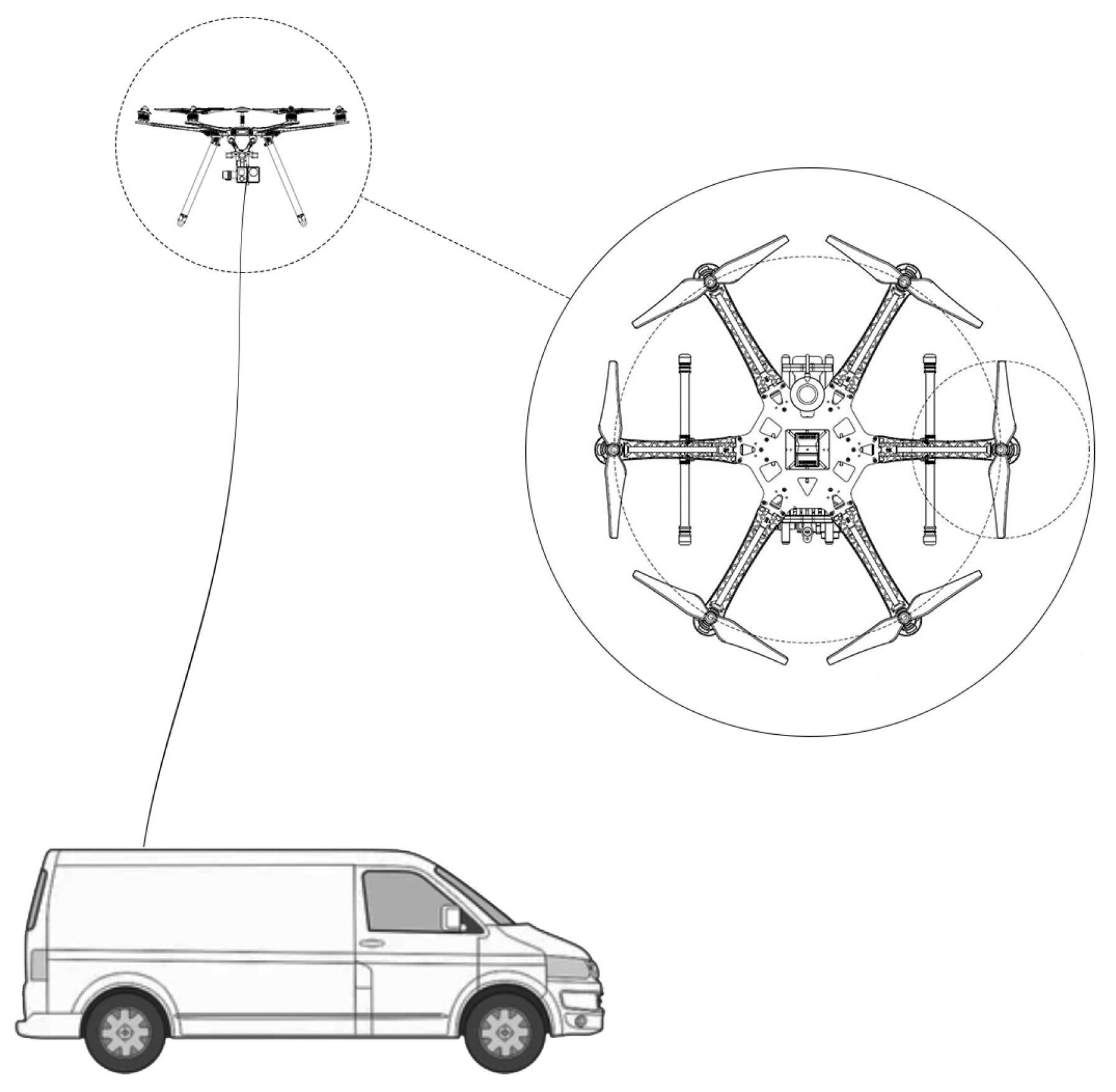
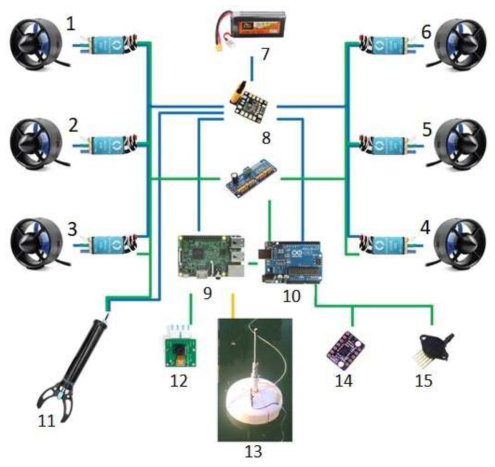
2.3.1. A Flight Module of a Tethered High-Altitude Telecommunication Platform

As an application example of the proposed k-out-of-n model, consider the model of a multi-copter flight module, which is part of the tethered high-altitude telecommunications platform [13]. The main area of its application is solving problems related to the long-term operation (tens of hours) without lowering the unmanned flight module to the ground. Therefore, unlike autonomous Unmanned Aerial Vehicles (UAVs) reliability parameters are of crucial importance for the tethered UAV-based high-altitude platforms.

A multi-rotor UAV is a system consisting of n rotors arranged uniformly in a circle and pairwise symmetrically with respect to the center of the circle [29]. The multi-copter may malfunction due to the failure of the propeller engines. There are various modifications of multi-rotor UAVs. The most common architectures are quad-, hexa-, and octocopters. The higher the redundancy ratio, the higher the reliability of the system. Therefore, in practice, flight modules with 6 or 8 rotors are most often used. In this example, we consider a hexacopter as a hot standby system consisting of $n=6$ components (rotors) that work and fail independently of each other (see Figure 1).

If the location of the failing components is not taken into account, this system fails when $k=2$ out of 6 rotors fail.For practical use, various reliability characteristics of such a system, including those considered in the general model, are of interest.

2.3.2. An Automated System for Remote Monitoring of a Sub-Sea Pipeline

As another application example of the k-out-of-n model, we consider an automated system for remote monitoring of a sub-sea pipeline. This system has been considered in [12], where its description has been given in details. One of the main parts of this system is an Unmanned Underwater Vehicle (UUV), the structure of which is illustrated in Figure 2.

The UUV consist of 6 motors, indicated by numbers 1–6, which allow it to rise, fall and move in various directions, including along the pipeline. The UUV is equipped with various devices, indicated by numbers 7–15, for receiving and transmitting information about the state of the pipe. In paper [12] the reliability function of this model has been studied in two scenarios:

(1)

in the case, when the system’s failure depends only on the number of its failed components. At that point, it is assumed that the device can perform its functions until at least 3 of its engines fail;

(2)

in the case, when the system’s failure depends also on the position of the failed components in the system. At that point, the UUV can perform its functions as long as at least two engines located on opposite sides, or any three engines are operational. Therefore, it could be considered to be a combination of $3+1$-out-of-$6:F$ and 5-out-of-$6:F$ systems. For such a system, the  special notation such as $(5,3+1)$-out-of-$6:F$ system was used.

However, the influence of the number of failed components on the residual lifetimes of the survived ones was not taken into account earlier. In the current paper, this model has been studied under the condition that failed components reduce the residual lifetime of surviving system’s components.

3. Distribution of the System’s Time to Failure

3.1. Preliminaries

It is evident that if a k-out-of-n system’s failure depends only on several its failed components, it coincides with the k-th order statistic from n iid rv $A_i(i=\overline{1,n})$ with a given cdf $A\left(t\right)$. For simplicity, further we will denote order statistics $A_{\left(1\right)}\le \cdots \le A_{\left(k\right)}\le \cdots \le A_{\left(n\right)}$ of iid rv $A_i(i=\overline{1,n})$ by $X_i$, i.e., $X_i=A_{\left(i\right)}$ and $X_1\le \cdots \le X_k\le \cdots \le X_n$. Distributions of order statistics are well studied (see, for example, [30]), where it was shown that the joint probability density function (pdf) $f_n(x_1,\dots x_n)$ of all order statistics $X_1\le X_2\le \cdots \le X_n$ from n iid rv $A_1,A_2,\dots ,A_n$ with a given pdf $a\left(x\right)$ has the following form:

$$f_n(x_1,x_2,\dots ,x_n)=n!a\left(x_1\right)a\left(x_2\right)\cdots a\left(x_n\right)(x_1\le x_2\le \cdots \le x_n).$$

By integration of this pdf with respect to last $n-k$ variables one can simply find the joint pdf $f_k(x_1,\dots x_k)$ of the first k order statistics $X_1\le X_2\le \cdots \le X_k$ from the n iid rv $A_i(i=\overline{1,n})$ in the domain $x_1\le x_2\le \dots \le x_k$ in the form

$$f_k(x_1,x_2,\dots ,x_k)=\frac{n!}{(n-k)!}a\left(x_1\right)a\left(x_2\right)\dots a\left(x_k\right){(1-A\left(x_k\right))}^{n-k}.$$

(1)

However, if a failure of one of the system’s components leads to the change in the residual lifetimes of all survived components, then their distributions are also changed.

3.2. Transformation of Order Statistics

Following the proposed model of the influence of components’ failures on the residual lifetime of survivors, they are reduced by multiplying by some constant $c_i$ depending on the number of failed components. Denote by $Y_i(i=\overline{1,k})$ the time of an i-th component failure under the conditions of increasing the load on survived components. To  simplify the representation of these values in terms of order statistics $X_1\le X_2\le \cdots \le X_n$, we introduce the following notations,

$$C_1=(1-c_1),C_2=c_1(1-c_2),\dots ,C_{k-1}=c_1\cdots c_{k-2}(1-c_{k-1}),C_k=c_1\cdots c_{k-1}.$$

In these notations, the following theorem holds.

Theorem 1. 

The time to the considered system failure $Y_k$ is a linear function of order statistics of the following form:

$$\begin{array}{c}\hfill Y_k=C_1{X}_1+C_2{X}_2+\cdots +C_{k-1}{X}_{k-1}+C_k{X}_k.\end{array}$$

(2)

Proof. 

To calculate the time of the system failure, we slightly expand the problem statement and calculate the successive time moments $Y_i(i=\overline{1,k})$ of failures of the system’s components under conditions of increasing load on the surviving components. To do that, we use a recursive procedure and denote by $X_i^{\left(j\right)}$ the expected time moment of the i-th failure after the failure of the j-th component $(i>j)$.

Thus, to start the induction, we have $X_i^{\left(0\right)}=X_i$. After the first failure of a component at time $Y_1=X_1^{\left(0\right)}=X_1$ all residual lifetimes of surviving components that equal $X_i-X_1$ for $i>1$ decrease by a factor of $c_1$, and therefore the expected failure times $X_i^{\left(1\right)}$ for $i>1$ take the form

$$\begin{array}{ccc}\hfill X_i^{\left(1\right)}& =& X_1^{\left(0\right)}+c_1(X_i^{\left(0\right)}-X_1^{\left(0\right)})=(1-c_1)X_1+c_1{X}_i,i=\overline{2,k}.\hfill \end{array}$$

Therefore $Y_2=X_2^{\left(1\right)}=(1-c_1)X_1+c_1{X}_2.$

Similarly, after the j-th failure at time $Y_j=X_j^{(j-1)},$ the residual lifetimes $X_i^{(j-1)}-X_j^{(j-1)}$ of all surviving components for all $i>j$ decrease by a factor $c_j,0<c_j<1$ ($j=\overline{1,k}$) and the expected failure times of components take the following form:

$$\begin{array}{ccc}\hfill X_i^{\left(j\right)}& =& X_i^{(j-1)},\forall i\le j,\hfill \\ \hfill X_i^{\left(j\right)}& =& X_j^{(j-1)}+c_j(X_i^{(j-1)}-X_j^{(j-1)})=(1-c_j)X_j^{(j-1)}+c_j{X}_i^{(j-1)},\forall i>j.\hfill \end{array}$$

Thus, the expected failure times of the system components $Y_j(j=\overline{1,k})$ under conditions of load redistribution equal to $Y_j=X_j^{(j-1)}(j=\overline{1,k})$. Expressing $X_i^{\left(j\right)}$ in terms of the original order statistics, we obtain the following expression for $i>j$:

$$\begin{array}{ccc}\hfill X_i^{\left(j\right)}& =& (1-c_1)X_1+c_1(1-c_2)X_2+c_1{c}_2(1-c_3)X_3+\cdots +c_1\cdots c_{j-1}(1-c_j)X_j+c_1\cdots c_j{X}_i\hfill \\ & =& \sum _{l=1}^j{c}_1\cdots c_{l-1}(1-c_l)X_l+c_1\cdots c_j{X}_i.\hfill \end{array}$$

(3)

Supposing that the last expression is true for a given j check it for all $i>j$:

$$\begin{array}{ccc}\hfill X_i^{(j+1)}& =& (1-c_1)X_1+c_1(1-c_2)X_2+c_1{c}_2(1-c_3)X_3+\cdots +c_1·\dots ·c_{j-1}(1-c_j)X_j\hfill \\ & +& c_1·\dots ·c_j(1-c_{j+1})X_{j+1}+c_1·\dots ·c_j{c}_{j+1}{X}_i\hfill \\ & =& \sum _{l=1}^j{c}_1\cdots c_{l-1}(1-c_l)X_l+c_1\cdots c_j(1-c_{j+1})X_{j+1}+c_1\cdots c_{j+1}{X}_i\hfill \\ & =& \sum _{l=1}^{j+1}{c}_1\cdots c_{l-1}(1-c_l)X_l+c_1\cdots c_{j+1}{X}_i.\hfill \end{array}$$

(4)

Hence, by the principle of mathematical induction, the equality (3) holds for any j. In terms of the original order statistics $X_i(i=\overline{1,k})$, we obtain for all $j=\overline{1,k}$:

$$Y_j=X_j^{(j-1)}=(1-c_1)X_1+c_1(1-c_2)X_2+\cdots +c_1\cdots c_{j-2}(1-c_{j-1})X_{j-1}+c_1\cdots c_{j-1}{X}_j,$$

which, using the notation introduced earlier, leads to (2) for $j=k$, which completes the proof.    □

3.3. Distribution of the System Failure Time

Now move on to the calculation of the cdf $F_{Y_k}\left(y\right)$ of the system’s time to failure $Y_k$ under the condition of redistribution of the load on the components. We will do that by taking into account expression (2) for the time of the system failure in terms of order statistics $X_i$ and using Formula (1) for the joint distribution of the first k order statistics.

To simplify the representation of this cdf we introduce the following notations,

$$\begin{array}{ccc}\hfill z_0& =& y,\hfill \\ \hfill z_i& =& z_i(y;x_1,\dots ,x_i)=\frac{y-C_1{x}_1+C_2{x}_2-\dots -C_i{x}_i}{C_{i+1}}(i=\overline{1,k-1}).\hfill \end{array}$$

(5)

With these notations the following theorem holds.

Theorem 2. 

The distribution of the system’s time to failure for $y>0$ is

$$\begin{array}{ccc}\hfill & & F_{Y_k}\left(y\right)=\mathbf{P}\{Y_k<y\}\hfill \\ & =& \frac{n!}{(n-k)!}\underset{0}{\overset{z_0}{\int }}a\left(x_1\right)d{x}_1\underset{x_1}{\overset{z_1}{\int }}a\left(x_2\right)d{x}_2\cdots \underset{x_{k-1}}{\overset{z_{k-1}}{\int }}a\left(x_k\right){(1-A\left(x_k\right))}^{n-k}d{x}_k.\hfill \end{array}$$

(6)

Proof. 

According to Theorem 1 (see Formula (2)) the time $Y_k$ of the system failure is the linear function of the first k order statistics

$$\begin{array}{c}\hfill Y_k=C_1{X}_1+C_2{X}_2+\cdots +C_{k-1}{X}_{k-1}+C_k{X}_k.\end{array}$$

Therefore, for cdf $F_{Y_k}\left(y\right)$ of rv $Y_k$ in terms of pdf $f_k(x_1,\dots ,x_k)$ of the first k order statistics we obtain

$$\begin{array}{ccc}\hfill F_{Y_k}\left(y\right)& =& \mathbf{P}\{Y_k<y\}\hfill \\ & =& \mathbf{P}\{C_1{X}_1+C_2{X}_2+\cdots +C_{k-1}{X}_{k-1}+C_k{X}_k<y\}\hfill \\ & =& \underset{D(x_1,\dots ,x_k;y)}{\int \cdots \int }{f}_k(x_1,x_2,\dots ,x_k)d{x}_1\dots d{x}_k,\hfill \end{array}$$

(7)

where the integration domain is

$$D(x_1,\dots ,x_k;y)=\{0\le x_1\le \cdots \le x_k,C_1{x}_1+C_2{x}_2+C_3{x}_3+\dots +C_{k-1}{x}_{k-1}+C_k{x}_k\le y\}.$$

Let us represent this multidimensional integral as an iterated one. Taking into account that $x_1\le x_2\le \cdots \le x_k$, the integration domain can be transformed in the following way. For the last variable $x_k$ from the inequality

$$C_1{x}_1+C_2{x}_2+C_3{x}_3+\dots +C_{k-1}{x}_{k-1}+C_k{x}_k\le y,$$

it follows that

$$x_k\le \frac{y-C_1{x}_1-C_2{x}_2-C_3{x}_3-\dots -C_{k-1}{x}_{k-1}}{c_1\cdots c_{k-1}}=z_{k-1}(y;x_1\dots x_{k-1}).$$

Furthermore, taking into account that $x_{k-1}\le x_k$, from the last inequality, it follows that

$$x_{k-1}\le x_k\le \frac{y-C_1{x}_1-C_2{x}_2-C_3{x}_3-\dots -C_{k-1}{x}_{k-1}}{c_1\cdots c_{k-1}}.$$

From this inequality with the simple algebra one can find

$$x_{k-1}\le \frac{y-C_1{x}_1-C_2{x}_2-\dots -C_{k-2}{x}_{k-2}}{c_1\cdots c_{k-2}}=z_{k-2}(y;x_1\dots ,x_{k-2}).$$

Following in the same way we obtain for variable $x_2$ the inequality

$$\begin{array}{ccc}\hfill y& \ge & (1-c_1)x_1+c_1(1-c_2)x_2+c_1{c}_2{x}_3\hfill \\ & \ge & (1-c_1)x_1+c_1(1-c_2)x_2+c_1{c}_2{x}_2=(1-c_1)x_1+c_1{x}_2,\hfill \end{array}$$

from which it follows that

$$x_2\le \frac{y-(1-c_1)x_1}{c_1},$$

and, at last,

$$y\ge (1-c_1)x_1+c_1{x}_1=x_1.$$

It means that $0\le x_1\le y$. This argumentation shows that the integration domain $D(x_1,\dots ,x_k;y)$ in terms of notations (5) can be represented as

$$D(x_1,\dots ,x_k;y)=\{x_{i-1}\le x_i\le z_i(y;x_1,\dots x_{i-1})(i=\overline{1,k})\}.$$

Thus, using Formula (1) for pdf $f_k(x_1,\dots ,x_k)$ for the first k order statistics and the above form of the integration domain, we can rewrite integral (7) for $y\ge 0$ as

$$F_{Y_k}\left(y\right)=\frac{n!}{(n-k)!}\underset{0}{\overset{y}{\int }}a\left(x_1\right)d{x}_1\underset{x_1}{\overset{z_1}{\int }}a\left(x_2\right)d{x}_2\cdots \underset{x_{k-1}}{\overset{z_{k-1}}{\int }}a\left(x_k\right){(1-A\left(x_k\right))}^{n-k}d{x}_k,$$

that ends the proof.    □

As a consequence of the theorem, the main system reliability characteristics can be calculated.

Remark 1. 

Based on the distribution of the system’s time to failure, any other system’s reliability characteristics can be calculated, such as:

–

its reliability function $R\left(y\right)=1-F_Y\left(y\right)$;

–

its mean lifetime $\mathbf{E}\left[T\right]={\int }_0^{\infty }R\left(t\right)dt$;

–

its lifetime variation $\mathbf{var}\left[T\right]$.

3.4. A Special Case: Exponential Distribution

In a special case, when the system components’ $A_i(i=\overline{1,n})$ lifetimes have exponential ($Exp$) distribution with a parameter $\alpha$ the integral (6) can be calculated analytically, but the calculations are rather cumbersome. We show it for the given value of $k=2$. But for exponential distribution of the system components’ lifetime, we propose another approach for the system lifetime distribution. It is based on the memoryless property of any exponentially distributed rv.

Denote by $T_i$ the time interval between $i-1$-th and i-th components failures, $i=\overline{1,k-1}$ ($T_0=0$). Then due to the memoryless property of the exponential distribution the time to the k-th failure $Y_k$ is the sum

$$Y_k=T_1+T_2+\cdots +T_k,$$

of k independent exponentially distributed rv $T_i$ with parameters

$${\lambda }_1=n\alpha ,{\lambda }_i=c_1{c}_2\cdots c_{i-1}(n-i+1)\alpha ={\overline{c}}_i(n-i+1)\alpha ,i=\overline{2,k},$$

where for simplicity additional notations are used:

$${\overline{c}}_i=\left\{\begin{array}{cc}1,\hfill & i=1,\hfill \\ c_1\cdots c_{i-1},\hfill & i=\overline{2,k}.\hfill \end{array}\right.$$

The moment generating function (mgf) of the system’s lifetime in this case has the following form:

$${\varphi }_k\left(s\right)=\mathbf{E}\left[e^{-s{Y}_k}\right]=\prod _{1\le i\le k}\mathbf{E}\left[e^{-s{T}_i}\right]=\prod _{1\le i\le k}\frac{{\overline{c}}_i{\lambda }_i}{s+{\overline{c}}_i{\lambda }_i}.$$

To apply the above theorem and the proposed approach, let us consider the simplest example of a k-out-of-n model with $k=2$. In this case, suppose $c_1=c$. Thus, according to (1) the joint distribution of rv $X_{\left(1\right)},X_{\left(2\right)}$ is

$$f_2(x_1,x_2)=\frac{n!}{(n-2)!}a\left(x_1\right)a\left(x_2\right){(1-A\left(x_2\right))}^{n-2}=\frac{n!}{(n-2)!}{\alpha }^2{e}^{-\alpha x_1}{e}^{-(n-1)\alpha x_2}.$$

Calculate cdf $F_{Y_2}\left(y\right)$ of the rv $Y_2=(1-c)X_{\left(1\right)}+c{X}_{\left(2\right)}$,

$$\begin{array}{ccc}\hfill F_{Y_2}\left(y\right)& =& \mathbf{P}\{(1-c)X_{\left(1\right)}+c{X}_{\left(2\right)}<y\}=\mathbf{P}\left\{X_{\left(2\right)}<\frac{y-(1-c)X_{\left(1\right)}}{c}\right\}\hfill \\ & =& n(n-1){\alpha }^2\underset{0}{\overset{y}{\int }}{e}^{-\alpha x_1}d{x}_1\underset{x_1}{\overset{\frac{y-(1-c)x_1}{c}}{\int }}{e}^{-(n-1)\alpha x_2}d{x}_2\hfill \\ & =& 1+\frac{n-1}{nc-(n-1)}{e}^{-n\alpha y}-\frac{nc}{nc-(n-1)}{e}^{-\frac{(n-1)\alpha }{c}y},\hfill \end{array}$$

and therefore its pdf for $y\ge 0$ is

$$f_{Y_2}\left(y\right)=\frac{n(n-1)\alpha }{nc-(n-1)}\left(e^{-\frac{(n-1)\alpha }{c}y}-e^{-n\alpha y}\right).$$

Please note that this result holds for $c\ne (n-1)/n$ and in this case the distribution is a mixture of exponential distributions. The point $c=(n-1)/n$ is a singular point for which cdf of the rv $Y_2$ is the Erlang distribution,

$$F_{Y_2}\left(y\right)=1-e^{-n\alpha y}-n\alpha y{e}^{-n\alpha y},y>0,$$

with pdf

$$p_{Y_2}\left(y\right)=n^2{\lambda }^{2}y{e}^{-n\lambda y},y>0.$$

Remark 2. 

The singularity in the calculation of the cdf of the system’s lifetime arises because for some special values of the coefficient $c_i$ (here for $c=(n-1)/n$) the moment generating function of the system’s lifetime has multiple roots that leads to changing of the shape of distribution.

With the help of another approach one can find mgf of the system’s lifetime in the following form:

$${\varphi }_2\left(s\right)=\frac{n(n-1){\alpha }^2}{s^2+(2n-1)\alpha s+n(n-1){\alpha }^2}.$$

By expanding this expression into simple fractions, we find

$${\varphi }_2\left(s\right)={\displaystyle \frac{n(n-1)\alpha }{s+n\alpha }}-{\displaystyle \frac{n(n-1)\alpha }{s+(n-1)\alpha }},$$

then, by calculating the inverse function, we obtain

$$f_2\left(y\right)=n(n-1)\alpha \left(e^{-(n-1)\alpha y}-e^{-n\alpha y}\right),$$

which is the same as the result above for $c=1$.

The analytical calculations of the reliability characteristics are not always possible. Nevertheless, their numerical analysis in the wide domain of initial data is possible. Therefore, in the next section a procedure for the numerical calculation of different reliability characteristics of the considered system will be proposed. Furthermore, in Section 5 this procedure will be used for the numerical analysis of the model with some examples.

4. The General Calculation Procedure of the System Reliability Characteristics and Numerical Experiments

Based on the results of the previous section, the general procedure for the problem solution can be implemented with the help of the following algorithm (Algorithm 1).

Algorithm 1: General algorithm for calculation of reliability function

Beginning. Determine: Integers $n,k$, real $c_i(i=\overline{1,k})$, distribution $A\left(t\right)$ of the system components’ lifetime and its pdf. Step 1. Taking into account that the system’s failure moment $Y_k$ according to Formula (2) equals $$Y_k=C_1{X}_1+C_2{X}_2+\cdots +C_{k-1}{X}_{k-1}+C_k{X}_k,$$ calculate the following, $$C_i=\left\{\begin{array}{cc}1-c_i,\hfill & i=1,\hfill \\ c_1\cdots c_{i-1}(1-c_i)\hfill & i=\overline{2,k-1},\hfill \\ c_1\cdots c_{k-1}\hfill & i=k.\hfill \end{array}\right.$$ Step 2. Taking into account that according to Formula (1), the joint distribution density of first k order statistics $X_1\le X_2\le \cdots \le X_k$ holds $$f_{X_1{X}_2\dots X_k}(x_1,x_2,\dots ,x_k)=\frac{n!}{(n-k)!}a\left(x_1\right)a\left(x_2\right)\dots a\left(x_k\right){(1-A\left(x_k\right))}^{n-k},$$ with which following to (6) calculate the reliability function $$\begin{array}{c}\hfill R\left(y\right)=1-F_{Y_k}\left(y\right)=1-\frac{n!}{(n-k)!}\underset{0}{\overset{y}{\int }}a\left(x_1\right)d{x}_1\underset{x_1}{\overset{z_1}{\int }}a\left(x_2\right)d{x}_2\cdots \underset{x_{k-1}}{\overset{z_{k-1}}{\int }}a\left(x_k\right){(1-A\left(x_k\right))}^{n-k}d{x}_k,\end{array}$$ where the limits of integration are determined by the relation (5) $$z_0=y,z_i=z_i(y;x_1,\dots ,x_i)=\frac{y-C_1{x}_1+C_2{x}_2-\dots -C_i{x}_i}{c_1{c}_2\dots c_i}(i=\overline{1,k-1}).$$ Find the values of the constants $c_i$ (singular points at which the denominator of the cdf $F_{Y_k}\left(y\right)$ turns into 0) for which the cdf changes its appearance. Step 3. From the system reliability function $R\left(y\right)$, calculate – mean time to the system failure $${\mu }_T=\mathbf{E}\left[Y_k\right]=\underset{0}{\overset{\infty }{\int }}R\left(y\right)dy;$$ – its variance $${\sigma }_T^2=\mathbf{Var}\left[Y_k\right]=\underset{0}{\overset{\infty }{\int }}{(y-{\mu }_T)}^{2}f\left(y\right)dy,\mathit{where}f\left(y\right)=\frac{d}{dy}{F}_{Y_k}\left(y\right),$$ and coefficient of variation $$v=\frac{\sigma }{\mu }.$$ Stop.

Remark 3. 

The algorithm can also be used to solve other different problems, for example, to analyze the sensitivity of the system’s reliability function and its characteristics to the shape of the lifetime distribution of the system’s components.

Furthermore, the algorithm will be applied to some examples.

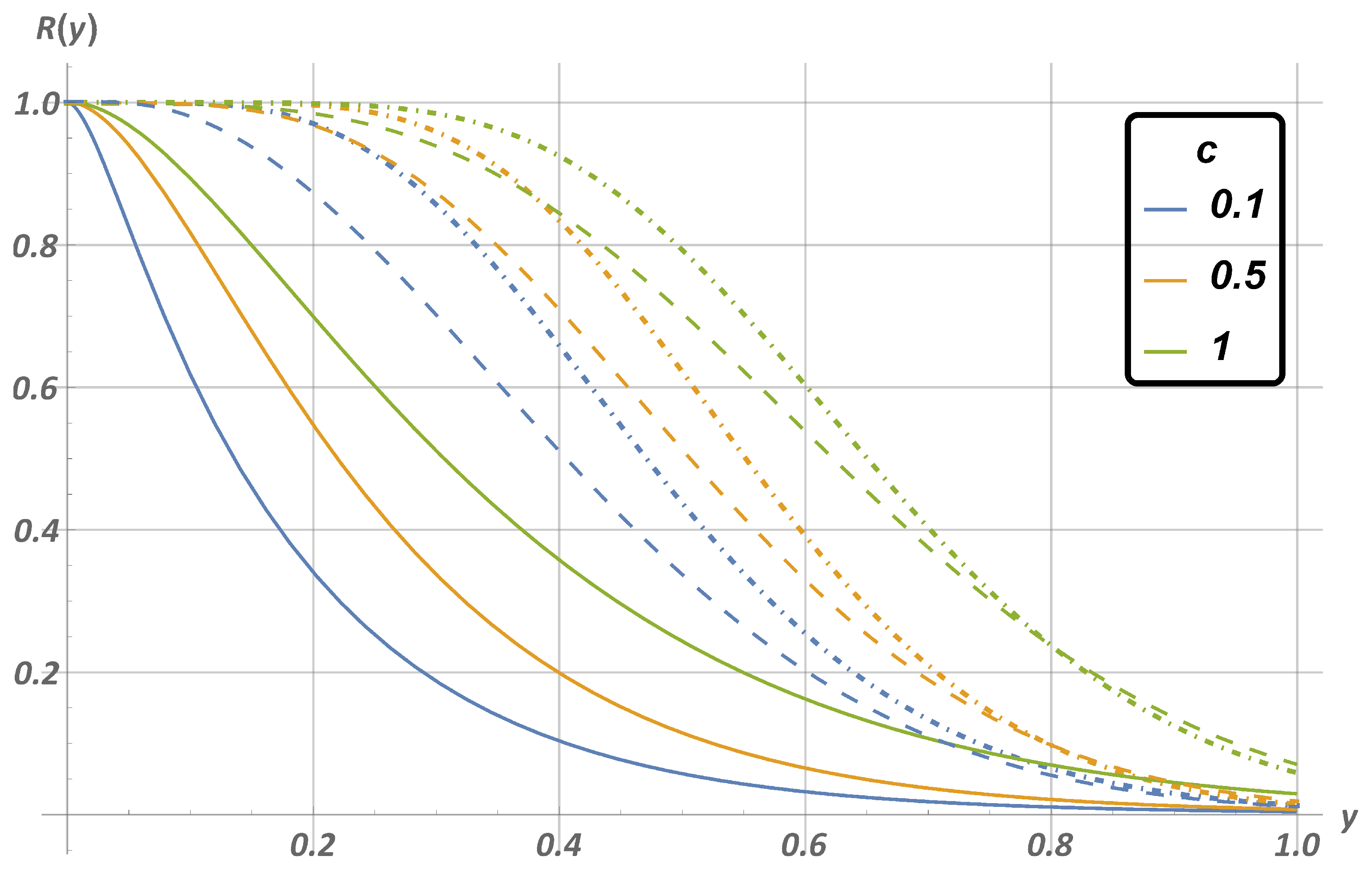
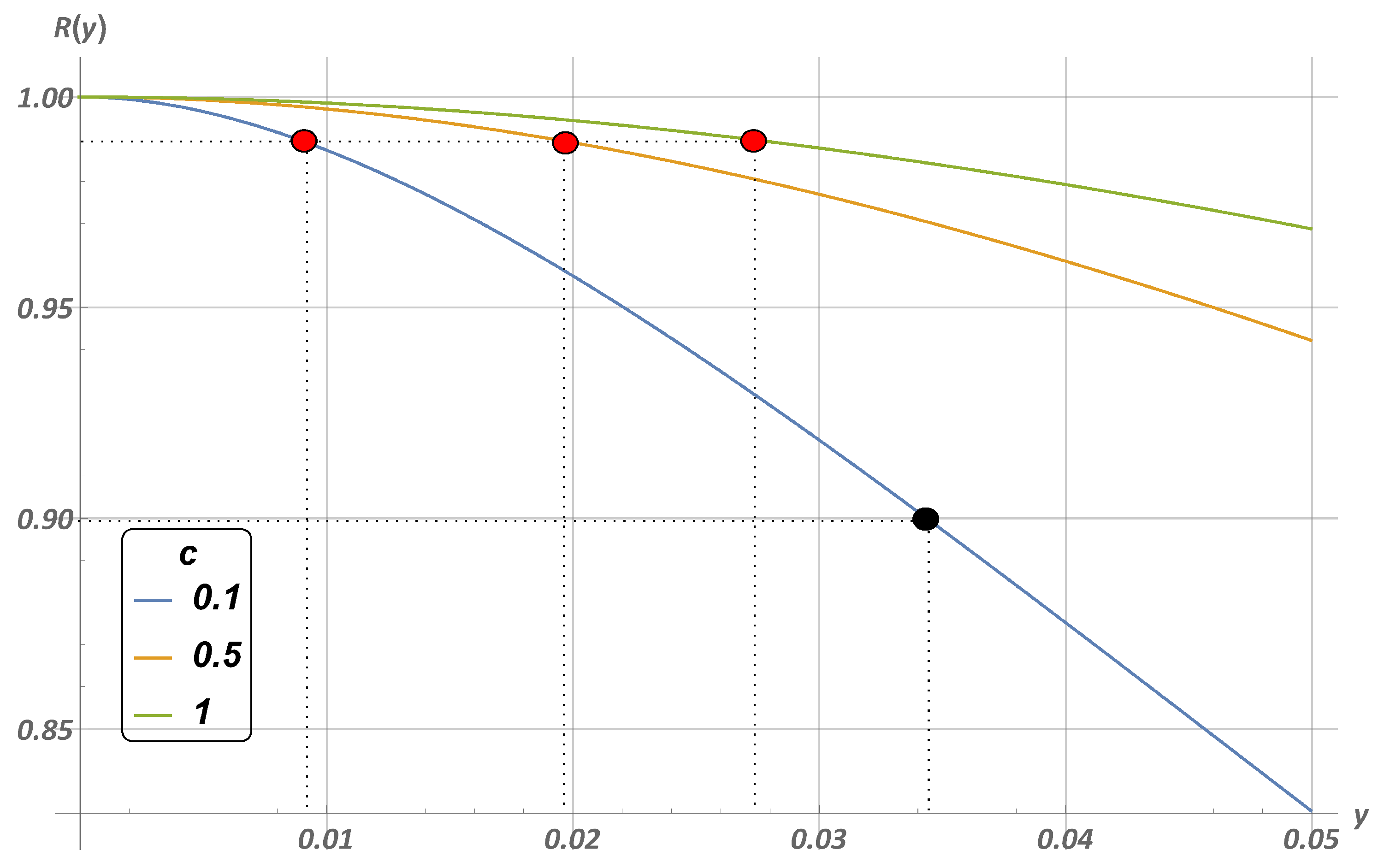
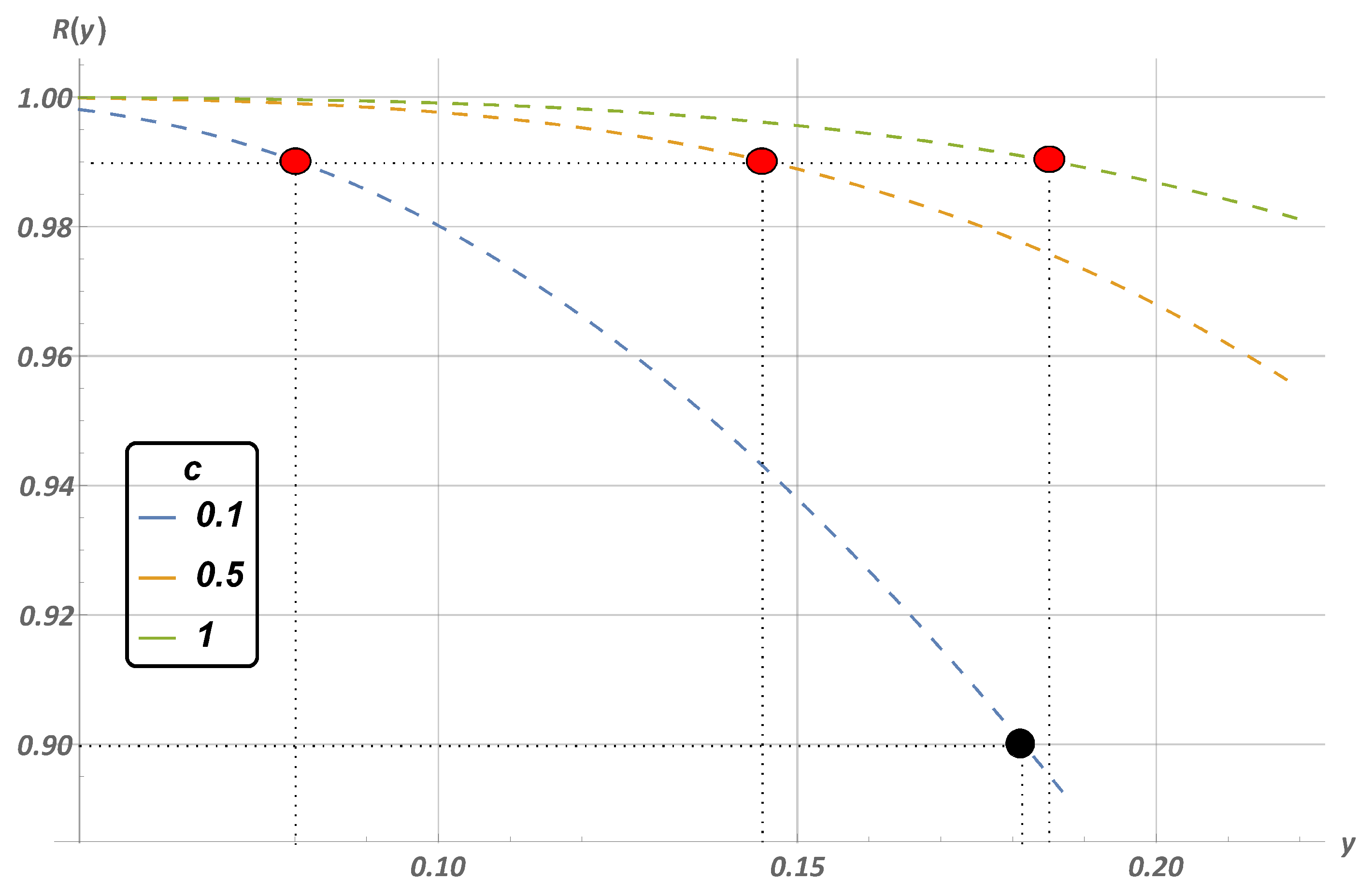
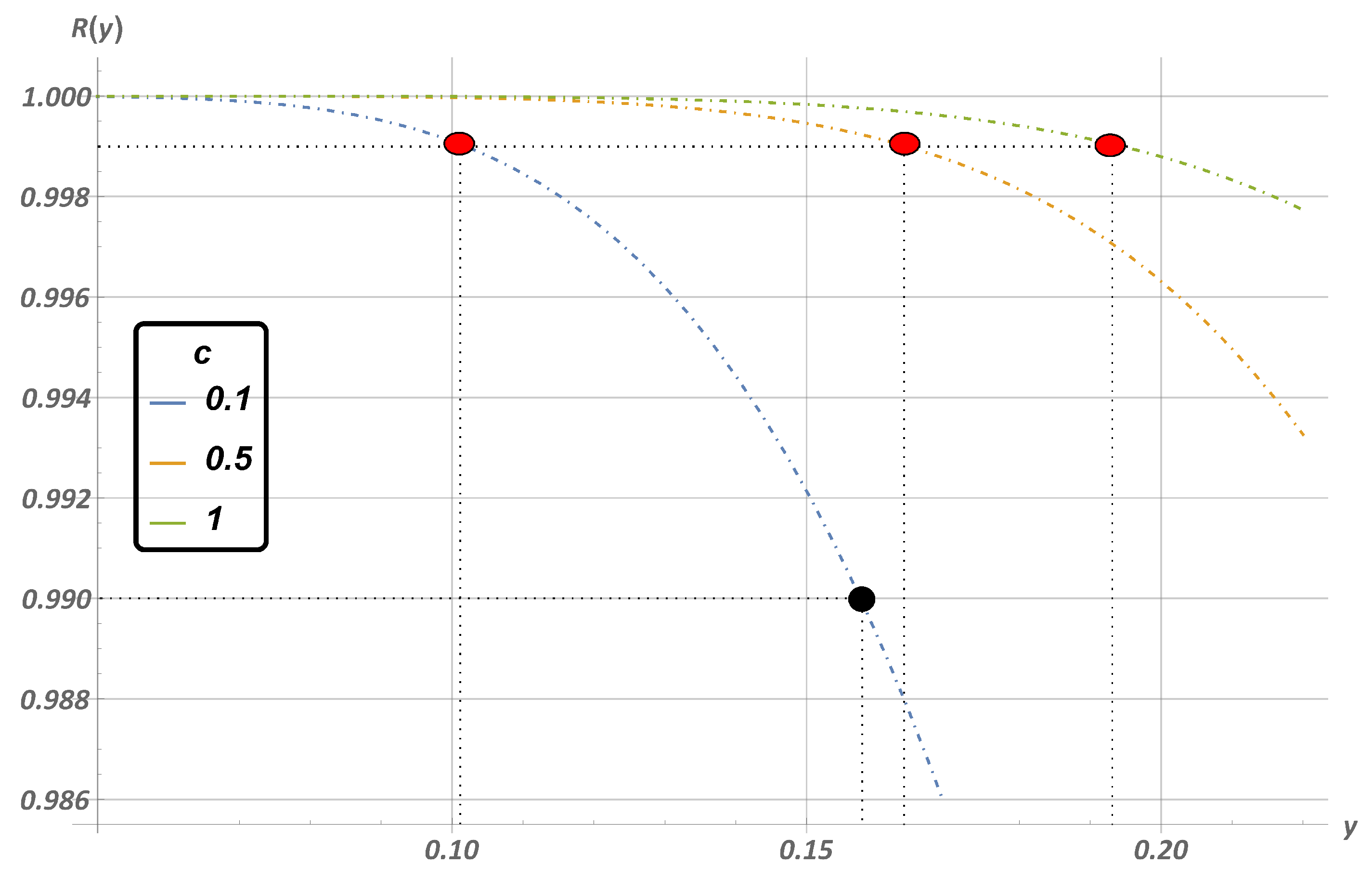
5. Numerical Experiments: 2-out-of-6 System

According to Algorithm 1, we calculate the reliability function of a 2-out-of-6 system. Since such a system fails due to the failure of two components, we have only one constant that defines the decreasing residual lifetime of surviving components. Therefore, hereafter, we suppose $c_1=c$. Consider the Gnedenko–Weibull ($GW$) distribution as the lifetime distribution of the system’s components, $A\left(t\right)\sim GW\left(\theta ,{\displaystyle \frac{a}{\mathsf{\Gamma }(1+{\theta }^{-1})}}\right)$, with the corresponding cdf

$$A\left(t\right)=1-exp\left\{-{\left({\displaystyle \frac{t\mathsf{\Gamma }(1+{\theta }^{-1})}{a}}\right)}^{\theta }\right\},t>0,$$

where

• a is a fixed mean components’ lifetime,
• $\theta$ is the shape parameter of $GW$ distribution calculated based on the preset value of the coefficient of variation,
• $v={\displaystyle \frac{\sigma }{a}}=a^{-1}·\sqrt{{\displaystyle \frac{\mathsf{\Gamma }(1+2·{\theta }^{-1})}{\mathsf{\Gamma }{(1+{\theta }^{-1})}^2}}-1}$ is the coefficient of variation,
• $\sigma$ is the standard deviation.

Additionally, consider the Erlang ($Erl$) distribution, $A\left(t\right)\sim Erl\left(l,\theta \right)$ with pdf

$$a\left(y\right)={\displaystyle \frac{{\theta }^l}{\mathsf{\Gamma }\left(l\right)}}{y}^{l-1}{e}^{-\theta y},y>0.$$

In this case, the distribution’s parameters can be represented via the corresponding mean a and coefficient of variation v as follows,

$$l=v^{-2},\theta ={\left(a{v}^2\right)}^{-1}.$$

For numerical experiments, we consider the reliability function and its characteristics of a 2-out-of-6 system for given distributions with a fixed mean a and different values of v. Thus, we can analyze the influence of the coefficient of variation of the repair time on the reliability characteristics of the system. In other words, investigate its sensitivity.

Suppose that the mean lifetime of the component $a=1$. If $\theta =1$, $GW$ and $Erl$ distributions transform into the exponential one with the mean time a and the coefficient of variation $v=1$. In this case, its reliability function is

$$R\left(t\right)={\displaystyle \frac{5e^{-6t}-6c·e^{-\frac{5t}{c}}}{5-6c}}.$$

(8)

From Formula (8) it is clear that $c=\frac{5}{6}$ leads to changing of the shape of distribution.

Since calculating the coefficient $\theta$ for $GW$ through the value of v is quite difficult, we define the parameter $\theta$ so that $v\approx 0.5$. Moreover, if $\theta$ of $GW$ takes non-integer values, it is not always possible to obtain a closed-form reliability function $R\left(t\right)$ according to Algorithm 1 (the integrand takes a complex form). Therefore, define $\theta =2$, then, the coefficient of variation $v=0.5227$. For $Erl$ distribution, suppose that $v=0.5$, which leads to $\theta =4$.

Suppose $c=0.1;0.5;1$. Figure 3 illustrates the reliability function of the 2-out-of-6 system for different distributions, as well as c and v. Here, solid line means $v=1$ and reliability function (8), dashed one is for $GW$ with $v=0.5227$ and dash-dotted is for $Erl$ with $v=0.5$. The legend of the figure denotes the color of line for different c.

The figure shows that the higher reliability coincides with the lower value of v. The case $c=1$ means the absence of load from the failed components to the surviving ones, thus this case corresponds to the highest reliability for different v compared to the values $c<1$. Moreover, dependence of the reliability function curve on the shape of lifetime distribution is observed. On a small interval y, the system reliability as $A\sim Erl$ is higher than as $A\sim GW$ for each c, despite close values v. This may indicate the sensitivity of the reliability function not only to the shape of the lifetime distribution, but also to the corresponding value of the coefficient of variation.

According to the algorithm, we calculate other reliability characteristics of the 2-out-of-6 system (

Table 1. $\mathbf{E}\left[Y_2\right]$ of a 2-out-of-6 system.

	$\mathit{c}=0.1$	$\mathit{c}=0.5$	$\mathit{c}=1$
$v=0.5$ ($A\sim Erl$)	$0.4925$	$0.5670$	$0.6668$
$v=0.5227$ ($A\sim GW$)	$0.4316$	$0.5251$	$0.6420$
$v=1$ ($A\sim Exp$)	$0.1867$	$0.2667$	$0.3667$

and

Table 2. $v_{sys}$ of a 2-out-of-6 system.

	$\mathit{c}=0.1$	$\mathit{c}=0.5$	$\mathit{c}=1$
$v_{comp}=0.5$ ($A\sim Erl$)	$0.3802$	$0.3049$	$0.2986$
$v_{comp}=0.5227$ ($A\sim GW$)	$0.4813$	$0.3854$	$0.3641$
$v_{comp}=1$ ($A\sim Exp$)	$0.8993$	$0.7289$	$0.7100$

). These characteristics correspond to the system’s reliability behavior, shown in Figure 3. The lower value of v leads to the higher value of the system lifetime expectation $\mathbf{E}\left[Y_2\right]$, and the lower value of c leads to the lower value of $\mathbf{E}\left[Y_2\right]$. Moreover, as $v\approx 0.5$ the relative error between the considered distributions is $14.11\%$ for $c=0.1$, $7.98\%$ for $c=0.5$ and $3.86\%$ for $c=1$.

To distinguish coefficients of variation of the components and the whole system, denote them as $v_{comp}$ and $v_{sys}$, respectively. Thus, Table 2 shows the following. With a decrease in c, the coefficient of variation of the system $v_{sys}$ grows and tends to the value of the coefficient of variation of each system component $v_{comp}$. The increasing $v_{comp}$ leads to the increasing $v_{sys}$ for all distributions and c. Thus, the coefficient of variation of the system $v_{sys}$ confirms that as c tends to 0 and $v_{comp}$ tends to 1, variability with respect to the average lifetime of the system $\mathbf{E}\left[Y_2\right]$ grows.

Table 1 showed that with increasing c and $v\approx 0.5$, the mean system lifetime $\mathbf{E}\left[Y_2\right]$ is very close. However, Figure 3 shows that over a small interval y with these c and v, the reliability of the system has significant differences. This leads to the study the quantiles of the system reliability. This measure shows how long the system will be reliable with a fixed probability. The quantiles $q_{\gamma }=R^{-1}\left(\gamma \right)$ of the reliability function are presented in Figure 4, Figure 5 and Figure 6. In all cases, red bullets correspond to $\gamma =0.99$, whereas black bullets correspond to $\gamma =0.9$.

All the values for quantiles $\gamma =0.999;0.99;0.9$ are presented in

Table 3. Quantiles of reliability function $q_{\gamma }$.

		$\mathit{c}=0.1$	$\mathit{c}=0.5$	$\mathit{c}=1$
$q_{0.999}$	$A\sim Exp$	$0.0026$	$0.0059$	$0.0083$
	$A\sim GW$	$0.0419$	$0.0804$	$0.1027$
	$A\sim Erl$	$0.1019$	$0.1641$	$0.1945$
$q_{0.99}$	$A\sim Exp$	$0.0088$	$0.0192$	$0.0271$
	$A\sim GW$	$0.0804$	$0.1458$	$0.1859$
	$A\sim Erl$	$0.1576$	$0.2345$	$0.2784$
$q_{0.9}$	$A\sim Exp$	$0.0344$	$0.0691$	$0.0972$
	$A\sim GW$	$0.1813$	$0.2784$	$0.3517$
	$A\sim Erl$	$0.271$	$0.3574$	$0.424$

for different distributions. The values in the table show that for the presented quantiles $q_{\gamma }$, the shape of the lifetime distribution of the system’s components as well as its coefficient of variation play a critical role on the system’s reliability. Therefore, for example, as $c=0.1$ and $A\sim Erl$ a given reliability level $0.9$ will last about 8 times longer than for $c=0.1$ and $A\sim Exp$. At that for $q_{0.999}$, the difference for similar case is almost 40 times. As the coefficient c increases, this difference decreases for all values of the quantiles and lifetime distributions of the components. As $c=1$ this difference is reduced by about two times. Thus, even as $c=1$, which defines no changing in components’ residual lifetimes, the influence not only of the lifetime distribution of the components but also its coefficient of variation on the reliability of the system is huge. This once again confirms the sensitivity of the reliability characteristics of the k-out-of-n system to the shape of the lifetime distribution and the coefficient of variation of system’s components.

6. Conclusions and the Further Investigations

The reliability function of a new k-out-of-$n:F$ model is investigated, under the new assumptions that the failures of its components lead to the increase in the load on the remaining ones and, consequently, to the change in their residual lifetimes. To model the situation, we proposed a novel approach based on the transformation of the order statistics of the system components’ lifetimes, which is the new field of application of order statistics. An algorithm for calculation of the system’s reliability function and its moments has been developed. Numerical experiments for the special case of the considered model based on the real-world systems have been carried out. The experiments show an essential sensitivity of the model reliability function and its moments to the shapes of the lifetime distributions of the system’s components and their coefficient of variation.

Furthermore, it is proposed we extend this approach to the investigation of stationary characteristics of the model and consider its preventive maintenance, aiming to improve its reliability characteristics.

References

1. Trivedi, K.S. Probability and Statistics with Reliability, Queuing and Computer Science Applications, 2nd ed.; John Wiley & Sons: New York, NY, USA, 2016. [Google Scholar] [CrossRef]
2. Chakravarthy, S.R.; Krishnamoorthy, A.; Ushakumari, P.V. A k-out-of-n reliability system with an unreliable server and Phase type repairs and services: The (N, T) policy. J. Appl. Math. Stoch. Anal. 2001, 14, 361–380. [Google Scholar] [CrossRef] [Green Version]
3. Rykov, V.; Kozyrev, D.; Filimonov, A.; Ivanova, N. On Reliability Function of a k-out-of-n System with General Repair Time Distribution. Probab. Eng. Inf. Sci. 2020, 35, 885–902. [Google Scholar] [CrossRef]
4. Pascual-Ortigosa, P.; Sáenz-de-Cabezón, E. Algebraic Analysis of Variants of Multi-State k-out-of-n Systems. Mathematics 2021, 9, 2042. [Google Scholar] [CrossRef]
5. Zhang, T.; Xie, M.; Horigome, M. Availability and reliability of (k-out-of-(M+N)): Warm standby systems. Reliab. Eng. Syst. Saf. 2006, 91, 381–387. [Google Scholar] [CrossRef]
6. Gertsbakh, I.; Shpungin, Y. Reliability Of Heterogeneous ((k, r)-out-of-(n, m)) System. RTA 2016, 3, 8–10. [Google Scholar]
7. Ushakov, I. A universal generating function. Sov. J. Comput. Syst. Sci. 1986, 24, 37–49. [Google Scholar]
8. Ushakov, I. Optimal standby problem and a universal generating function. Sov. J. Comput. Syst. Sci. 1987, 25, 61–73. [Google Scholar]
9. Levitin, G. The Universal Generating Function in Reliability Analysis and Optimization; Springer Series in Reliability Engineering; Springer: London, UK, 2005. [Google Scholar] [CrossRef]
10. Kala, Z. New Importance Measures Based on Failure Probability in Global Sensitivity Analysis of Reliability. Mathematics 2021, 9, 2425. [Google Scholar] [CrossRef]
11. Rykov, V.; Sukharev, M.; Itkin, V. Investigations of the Potential Application of k-out-of-n Systems in Oil and Gas Industry Objects. J. Mar. Sci. Eng. 2020, 8, 928. [Google Scholar] [CrossRef]
12. Rykov, V.; Kochueva, O.; Farkhadov, M. Preventive Maintenance of a k-out-of-n System with Applications in Subsea Pipeline Monitoring. J. Mar. Sci. Eng. 2021, 9, 85. [Google Scholar] [CrossRef]
13. Vishnevsky, V.M.; Kozyrev, D.V.; Rykov, V.V.; Nguyen, D.P. Reliability modeling of an unmanned high-altitude module of a tethered telecommunication platform. Inf. Technol. Comput. Syst. 2020, 4, 26–36. [Google Scholar] [CrossRef]
14. Zhang, J.; Jiang, Y.; Li, X.; Huo, M.; Luo, H.; Yin, S. An adaptive remaining useful life prediction approach for single battery with unlabeled small sample data and parameter uncertainty. Reliab. Eng. Syst. Saf. 2022, 222, 108357. [Google Scholar] [CrossRef]
15. Zhang, J.; Jiang, Y.; Li, X.; Luo, H.; Yin, S.; Kaynak, O. Remaining Useful Life Prediction of Lithium-Ion Battery with Adaptive Noise Estimation and Capacity Regeneration Detection. IEEE/ASME Trans. Mechatron. 2022, 1–12. [Google Scholar] [CrossRef]
16. Zhang, J.; Jiang, Y.; Wu, S.; Li, X.; Luo, H.; Yin, S. Prediction of remaining useful life based on bidirectional gated recurrent unit with temporal self-attention mechanism. Reliab. Eng. Syst. Saf. 2022, 221, 108297. [Google Scholar] [CrossRef]
17. Eryilmaz, S. Phase type stress-strength models with reliability applications. Commun. Stat.—Simul. Comput. 2018, 47, 954–963. [Google Scholar] [CrossRef]
18. Bai, X.; Shi, Y.; Liu, Y.; Liu, B. Reliability estimation of stress-strength model using finite mixture distributions under progressively interval censoring. J. Comput. Appl. Math. 2019, 348, 509–524. [Google Scholar] [CrossRef]
19. Zhang, L.; Xu, A.; An, L.; Li, M. Bayesian inference of system reliability for multicomponent stress-strength model under Marshall-Olkin Weibull distribution. Systems 2022, 10, 196. [Google Scholar] [CrossRef]
20. Tang, Y.; Zhang, J. New model for load-sharing k-out-of-n : G system with different components. J. Syst. Eng. Electron. 2008, 19, 748–751, 842. [Google Scholar] [CrossRef]
21. Hellmich, M. Semi-Markov embeddable reliability structures and applications to load-sharing k-out-of-n system. Int. J. Reliab. Qual. Saf. Eng. 2013, 20, 1350007. [Google Scholar] [CrossRef]
22. Bairamov, I.; Arnold, B.C. On the residual lifelengths of the remaining components in an nk + 1 out of n system. Stat. Probab. Lett. 2008, 78, 945–952. [Google Scholar] [CrossRef]
23. Nguyen, D.P.; Kozyrev, D.V. Reliability Analysis of a Multirotor Flight Module of a High-altitude Telecommunications Platform Operating in a Random Environment. In Proceedings of the 2020 International Conference Engineering and Telecommunication (En&T), Dolgoprudny, Russia, 25–26 November 2020; pp. 1–5. [Google Scholar] [CrossRef]
24. Rykov, V.; Ivanova, N.; Kochetkova, I. Reliability Analysis of a Load-Sharing k-out-of-n System Due to Its Components’ Failure. Mathematics 2022, 10, 2457. [Google Scholar] [CrossRef]
25. Katzur, A.; Kamps, U. Order statistics with memory: A model with reliability applications. J. Appl. Probab. 2016, 53, 974–988. [Google Scholar] [CrossRef]
26. Cramer, E.; Kamps, U. Sequential order statistics and k-out-of-n systems with sequentially adjusted failure rates. Ann. Inst. Stat. Math. 1996, 48, 535–549. [Google Scholar] [CrossRef]
27. Navarro, J.; Marco, B. Coherent Systems Based on Sequential Order Statistics. Nav. Res. Logist. 2011, 58, 123–135. [Google Scholar] [CrossRef]
28. Sutar, S.; Naik-Nimbalkar, U.V. A load share model for non-identical components of a k-out-of-m system. Appl. Math. Model. 2019, 72, 486–498. [Google Scholar] [CrossRef]
29. Kozyrev, D.V.; Phuong, N.D.; Houankpo, N.G.K.; Sokolov, A. Reliability evaluation of a hexacopter-based flight module of a tethered unmanned high-altitude platform. Commun. Comput. Inf. Sci. 2019, 1141, 646–656. [Google Scholar] [CrossRef]
30. David, H.A.; Nagaraja, H.N. Order Statistics, 3rd ed.; John Wiley & Sons: New York, NY, USA, 2003. [Google Scholar] [CrossRef]
Figure 1. An unmanned hexacopter flight module of a tethered high-altitude telecommunications platform.
Mathematics 10 04243 g001
Figure 2. An unmanned multi-functional underwater vehicle.
Mathematics 10 04243 g002
Figure 3. Reliability function of a 2-out-of-6 system.
Mathematics 10 04243 g003
Figure 4. Reliability function with v = 1 and quantiles ( A E x p ). Red and black bullets are the points of intersection of the reliability function curves with fixed reliability levels of 0.99 and 0.9, respectively.
Mathematics 10 04243 g004
Figure 5. Reliability function with v = 0.5227 and quantiles ( A G W ). Red and black bullets are the points of intersection of the reliability function curves with fixed reliability levels of 0.99 and 0.9, respectively.
Mathematics 10 04243 g005
Figure 6. Reliability function with v = 0.5 and quantiles ( A E r l ). Red and black bullets are the points of intersection of the reliability function curves with fixed reliability levels of 0.99 and 0.9, respectively.
Mathematics 10 04243 g006