Convergence of Neural Networks with a Class of Real Memristors with Rectifying Characteristics

Abstract

The paper considers a neural network with a class of real extended memristors obtained via the parallel connection of an ideal memristor and a nonlinear resistor. The resistor has the same rectifying characteristic for the current as that used in relevant models in the literature to account for diode-like effects at the interface between the memristor metal and insulating material. The paper proves some fundamental results on the trajectory convergence of this class of real memristor neural networks under the assumption that the interconnection matrix satisfies some symmetry conditions. First of all, the paper shows that, while in the case of neural networks with ideal memristors, it is possible to explicitly find functions of the state variables that are invariants of motions, the same functions can be used as Lyapunov functions that decrease along the trajectories in the case of real memristors with rectifying characteristics. This fundamental property is then used to study convergence by means of a reduction-of-order technique in combination with a Lyapunov approach. The theoretical predictions are verified via numerical simulations, and the convergence results are illustrated via the applications of real memristor neural networks to the solution of some image processing tasks in real time.

1. Introduction

Nowadays, Von Neumann computing architectures are facing severe limitations in the handling of big data in the Internet of Things (IoT) and cloud computing systems in real time [1,2,3,4]. One of the main problems is the memory bottleneck that occurs because the central processing unit (CPU) and the memory (e.g., the RAM) have different physical locations. This implies that the time needed to handle the continuous transfer of data between the CPU and RAM may be excessively long, and the electronic power requirements may be demanding. The use of memristors and, more generally, emerging nanoscale memristive devices is a long-term vision with the aim of overcoming some of the limitations of Von Neumann computing architectures via the implementation of analog and parallel neuromorphic computing paradigms akin to some basic principles on which biological brains operate [5,6,7,8]. In particular, memristors enable the implementation of in-memory computing schemes in which the same device is used to compute as well as store the computational result, thus overcoming the Von Neumann memory bottleneck [9,10,11].

Memristors have been classified as ideal, generic, and extended memristors [12,13,14]. Ideal memristors, which were introduced in the seminal 1971 paper by Prof. Leon Chua [15], are defined by a nonlinear relation between the flux (the integral of voltage) and charge (the integral of current). In the voltage–current domain, an ideal voltage-controlled memristor satisfies a state-dependent Ohm’s law where the conductance (which is also called the memductance) is a function of the state, i.e., the flux. Ideal memristors continue to be of great interest in circuit theory. However, they are often inadequate for accurately modeling the switching behavior of real electronic memristive devices that are implemented in nanotechnology [16,17,18,19]. Currently, real devices need to be modeled using generic or extended memristors, which involve one or more state variables—not necessarily including the flux—and more general forms of the state-dependent Ohm’s law and state equations [13].

Convergence of trajectories toward equilibrium points (EPs) is one of the most relevant dynamical properties of a neural network (NN) from both a theoretical and an applied point of view. Convergent NNs may be used for the implementation of content-addressable memories (CAMs), where the information is stored in the stable EPs of the NN in order to solve combinatorial optimization problems in which the local minima of an associated energy function correspond to the optimal solutions of the problem and to solve several other signal processing tasks in real time [20,21,22,23,24,25]. Convergence of NNs has been widely investigated for traditional NNs without memristors by using various techniques, such as the Lyapunov method, the dichotomy of omega-limit sets for cooperative systems, the global consistency of the decision schemes implemented by competitive NNs, and the ojasiewicz inequality combined with the concept of trajectories with a finite length for NNs with analytic nonlinearities. The reader is referred to [20,22,26,27,28,29,30,31] and the references therein for an account of some of the main contributions on the convergence of NNs. On the other hand, only a few papers are available in the literature on the convergence of memristor neural networks (MNNs). The authors of [32,33,34] provided results on the convergence of MNNs with ideal memristors in the case of symmetric interconnections and in that of cooperative (non-negative) interconnections between neurons. There, convergence was studied by using the flux–charge analysis method (FCAM) and a reduction-of-order technique [14]. The authors of [35,36] established results on multistability for MNNs with ideal memristors while considering delays in the interconnections, and they also used FCAM. To the authors’ knowledge, so far, only very specific results have been obtained on the convergence of MNNs with real memristor devices. In this regard, we mention the paper [37], which established convergence for MNNs with a class of generic memristors obeying the VTEAM model, as well as [38], in which the convergence of a class of cellular MNNs with real memristors and second-order cells was analyzed.

In this paper, we consider MNNs with a class of extended memristors that were introduced in [39] and obtained via the parallel connection of an ideal voltage-controlled memristor and a voltage-controlled nonlinear resistor. These networks are named real memristor neural networks (RMNNs). The paper establishes some fundamental results on the trajectory convergence when the neuron interconnections are symmetric and the resistor nonlinearity satisfies some sector conditions. It is stressed that such a condition is met by relevant memristive device models that display rectifying properties for the current due to the diode-like behavior at the interface of the metal and the insulating material. The convergence of RMNNs was analyzed by using the Lyapunov approach in relation to equivalent systems written in the integral flux–charge domain. The main starting point was the property that, while MNNs with ideal memristors admit functions of the state variables that are invariants of motion, the same functions can be used as Lyapunov functions that decrease along the trajectories in the case of RMNNs with rectifying nonlinear resistors. Numerical simulations concerning RMNNs for image processing are presented in the paper to verify the theoretical results on convergence.

Notation: Given a column vector $x\in {\mathbb{R}}^n$, $x^{\top }$ refers to the transpose of x. We denote by $B(x,R)=\{y\in {\mathbb{R}}^n:\parallel y-x\parallel <R\}$ an open ball with radius $R>0$ centered at $x\in {\mathbb{R}}^n$. If $U\subset {\mathbb{R}}^n$, $\overline{U}$ is the closure of U, while $\partial U$ denotes the boundary of U.

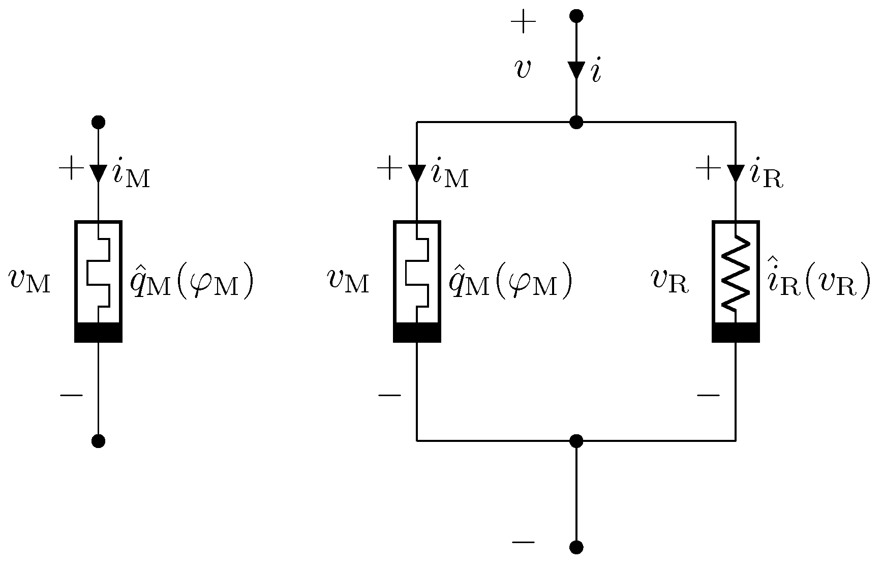
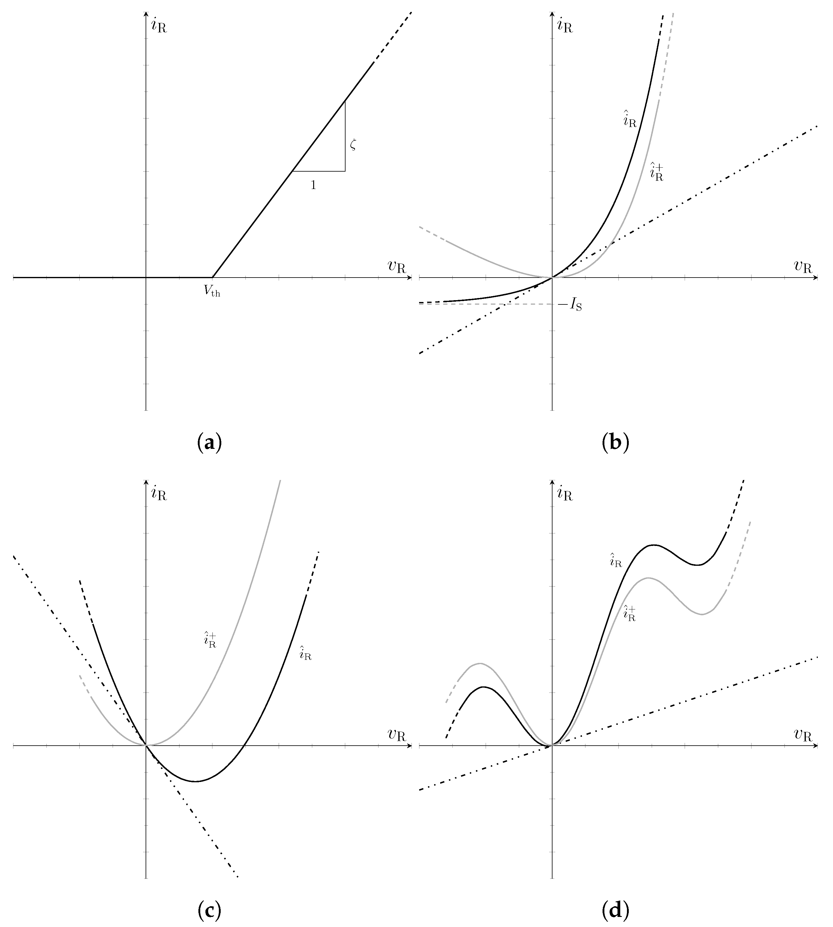
2. Memristor Models

Let $v_{\mathrm{M}}(t)$ (or $i_{\mathrm{M}}(t)$) be the voltage (or current) of the memristor (Figure 1). In addition, consider the flux ${\phi }_{\mathrm{M}}(t)={\int }_{-\infty }^t{v}_{\mathrm{M}}(\sigma )d\sigma$ and the charge $q_{\mathrm{M}}(t)={\int }_{-\infty }^t{i}_{\mathrm{M}}(\sigma )d\sigma$. An ideal flux-controlled memristor is defined by the constitutive relation $q_{\mathrm{M}}={\widehat{q}}_{\mathrm{M}}({\phi }_{\mathrm{M}})$, where ${\widehat{q}}_{\mathrm{M}}\in C^1(\mathbb{R})$ is the nonlinear flux–charge characteristic. Differentiating in time, we find that an ideal memristor satisfies the state-dependent Ohm’s law:

$$i_{\mathrm{M}}={\widehat{q}}_{\mathrm{M}}^{\prime }({\phi }_{\mathrm{M}})v_{\mathrm{M}}.$$

Note that the dot refers to the time derivative, while the prime is used to denote the derivative of a function with respect to its argument. The state variable is the flux ${\phi }_{\mathrm{M}}$ and ${\widehat{q}}_{\mathrm{M}}^{\prime }({\phi }_{\mathrm{M}})$ is the state-dependent memristor conductance, which is also called the memductance.

The authors of [39] introduced a class of real extended memristors obtained through the parallel connection of an ideal flux-controlled memristor $q_{\mathrm{M}}={\widehat{q}}_{\mathrm{M}}({\phi }_{\mathrm{M}})$ and a nonlinear voltage-controlled resistor $i_{\mathrm{R}}={\widehat{i}}_{\mathrm{R}}(v_{\mathrm{R}})$, where $v_{\mathrm{R}}$ (or $i_{\mathrm{R}}$) is the voltage (or the current) in the resistor, ${\widehat{i}}_{\mathrm{R}}$ is locally Lipschitz in $\mathbb{R}$, and ${\widehat{i}}_{\mathrm{R}}(0)=0$ (Figure 1). Since $i=i_{\mathrm{M}}+i_{\mathrm{R}}$ and $v=v_{\mathrm{M}}=v_{\mathrm{R}}$, the extended memristor satisfies

$$i={\widehat{q}}_{\mathrm{M}}^{\prime }(\phi )v+{\widehat{i}}_{\mathrm{R}}(v)$$

(1)

where

$$\dot{\phi }={\dot{\phi }}_{\mathrm{M}}=v.$$

In this paper, we consider one of the next hypotheses.

Assumption 1.

We have ${\widehat{i}}_{\mathrm{R}}(v_{\mathrm{R}})\ge 0$ for any $v_{\mathrm{R}}\in \mathbb{R}$.

Assumption 2.

There exists $\gamma \ge 0$ such that the function ${\widehat{i}}_{\mathrm{R}}^{+}(v_{\mathrm{R}})\doteq {\widehat{i}}_{\mathrm{R}}(v_{\mathrm{R}})-\gamma v_{\mathrm{R}}$ satisfies Assumption 1.

Clearly, Assumption 1 is more restrictive than Assumption 2. In addition, note that if ${\widehat{i}}_{\mathrm{R}}\in C^1(\mathbb{R})$, Assumption 2 is equivalent to ${\widehat{i}}_{\mathrm{R}}(v)-{\widehat{i}}_{\mathrm{R}}^{\prime }(0)v\ge 0$ for any $v\in \mathbb{R}$.

Consider, for example, the diode-like piecewise-linear (PWL) function

$${\widehat{i}}_{\mathrm{R}}(v_{\mathrm{R}})=\left\{\begin{array}{cc}0,\hfill & v_{\mathrm{R}}<V_{\mathrm{th}}\hfill \\ \zeta v_{\mathrm{R}},\hfill & v_{\mathrm{R}}\ge V_{\mathrm{th}}\hfill \end{array}\right.$$

(2)

where $V_{\mathrm{th}}>0$ is the diode threshold voltage and $\zeta >0$ is the differential conductance when the diode is turned on (Figure 2a). The PWL characteristic (2), which satisfies Assumption 1, is used as an approximation of the Shockley model of a diode given by

$${\widehat{i}}_{\mathrm{R}}(v_{\mathrm{R}})=I_{\mathrm{S}}\left(exp\left(\frac{v_R}{\eta V_{\mathrm{T}}}\right)-1\right)$$

(3)

where $I_{\mathrm{S}}$ is the reverse bias saturation current, $V_{\mathrm{T}}$ is the thermal voltage, and $\eta$ is the ideality factor (Figure 2b). Note that the characteristic (3) satisfies Assumption 2 and ${\widehat{i}}_{\mathrm{R}}^{+}(v_{\mathrm{R}})=i_{\mathrm{R}}(v_{\mathrm{R}})-(I_{\mathrm{S}}/\eta V_{\mathrm{T}})v_{\mathrm{R}}$. Two more nonlinearities that satisfy Assumption 2 are depicted in Figure 2c,d.

Rectifying the resistor characteristics of the type introduced here is of importance in the modeling of real memristor devices. As a relevant example, the authors of [40] introduced a model with a parallel connection of a memristor and a diode, with the latter accounting for the rectification effect in the off-state due to the Schottky-like transport at one of the metal/oxide memristor interfaces. Several analogous models of barrier-type memristors in which a diode-like nonlinear resistor was introduced for better modeling of the experimentally observed pinched hysteresis loops in response to a zero-mean sinusoidal excitation were reviewed, for instance, in [41,42].

When subjected to a zero-mean sinusoidal input, an ideal memristor displays a hysteresis loop in the voltage–current plane that is symmetric about the origin. It was demonstrated in [39] that, through suitable massaging, the nonlinear resistor characteristic model (1) is capable of reproducing nonsymmetric hysteresis loops that can be observed for some classes of real memristor devices. On the other hand, it should be noted that model (1) has the memristor flux as the internal state variable, as it happens for a flux-controlled ideal memristor. Other types of memristors do not necessarily admit the flux as a state variable, or they may have additional state variables, such as the temperature or geometric quantities that characterize the insulating or conductive part. Finally, it is remarked that model (1) describes a nonvolatile memristor, while some classes of real memristors are volatile, such as thermistors [12].

3. Memristor Neural Network Models

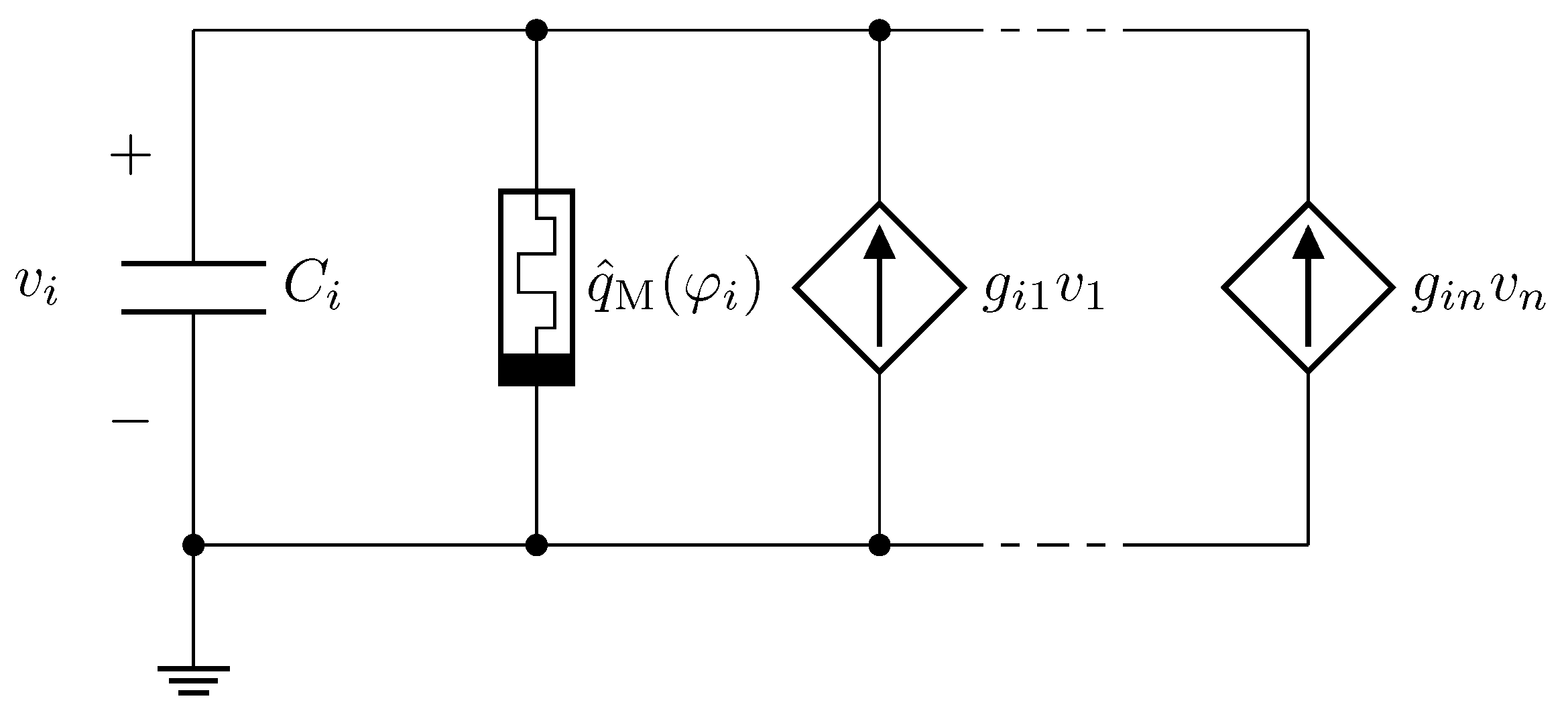
3.1. Ideal Memristor Neural Network Model

The authors of [32,33,35,36,43] considered an array of n interconnected dynamical cells with a structure of an NN. The circuit schematic of a cell is depicted in Figure 3. The i-th cell is obtained via the parallel connection of an ideal capacitor $C>0$ and an ideal flux-controlled memristor $q_i={\widehat{q}}_{\mathrm{M}}({\phi }_i)$, that is, the cell is obtained by replacing the linear resistor in a typical cellular neural network (CNN) cell with a memristor (compare Figure 3 with ([23], Figure 3)). This array is called an ideal memristor neural network (IMNN). It is observed that in the cell of Figure 3, the only nonlinearity is the memristor, while in a CNN, the nonlinearity corresponds to the piecewise-linear input-voltage/output-voltage characteristic implemented by an operational amplifier. The interconnection of the j-th cell, $j=1,\dots ,n$, with the i-th cell is obtained by means of a linear conductance $g_{ij}$. Actually, $v_j$ is sensed via an operational amplifier operating as a buffer, and a voltage-controlled current source (VCCS) is used to inject the current $g_{ij}{v}_j$ into the i-th cell. A possible circuit implementation of the buffer and VCCS is discussed in the appendix of [23].

An IMNN satisfies the following system of differential equations:

$$\begin{array}{cc}\hfill C{\dot{v}}_i& =-{\widehat{q}}_{\mathrm{M}}^{\prime }({\phi }_i)v_i+\sum _{j=1}^n{g}_{ij}{v}_j\hfill \\ \hfill {\dot{\phi }}_i& =v_i\hfill \end{array}$$

(4)

for $i=1,\dots ,n$. In vector form, we have

$$\begin{array}{cc}\hfill C\dot{v}& =-{\widehat{Q}}_{\mathrm{M}}^{\prime }(\phi )v+Gv\hfill \\ \hfill \dot{\phi }& =v\hfill \end{array}$$

(5)

where we let $v={(v_1,\dots ,v_n)}^{\top }\in {\mathbb{R}}^n$ and $Q_{\mathrm{M}}^{\prime }(\phi )=\mathrm{diag}({\widehat{q}}_{\mathrm{M}}^{\prime }({\phi }_1),\dots ,{\widehat{q}}_{\mathrm{M}}^{\prime }({\phi }_n))\in {\mathbb{R}}^{n\times n}$, and $G=[g_{ij}]\in {\mathbb{R}}^{n\times n}$ is the neuron interconnection matrix (the superscript ⊤ refers to the transpose). This is an autonomous system of $2n$ differential equations in the state variables $(v,\phi )\in {\mathbb{R}}^{2n}$.

Results on the convergence of solutions of (5) are given in [32] under the assumption that G is symmetric and in [33] when G has non-negative off-diagonal entries, while conditions ensuring multistability are obtained in [35,36]. The global stability of the EP of (5) was established in [43]. The results in these papers were obtained via a reduction-of-order technique and the use of the flux–charge analysis method developed in [14,44].

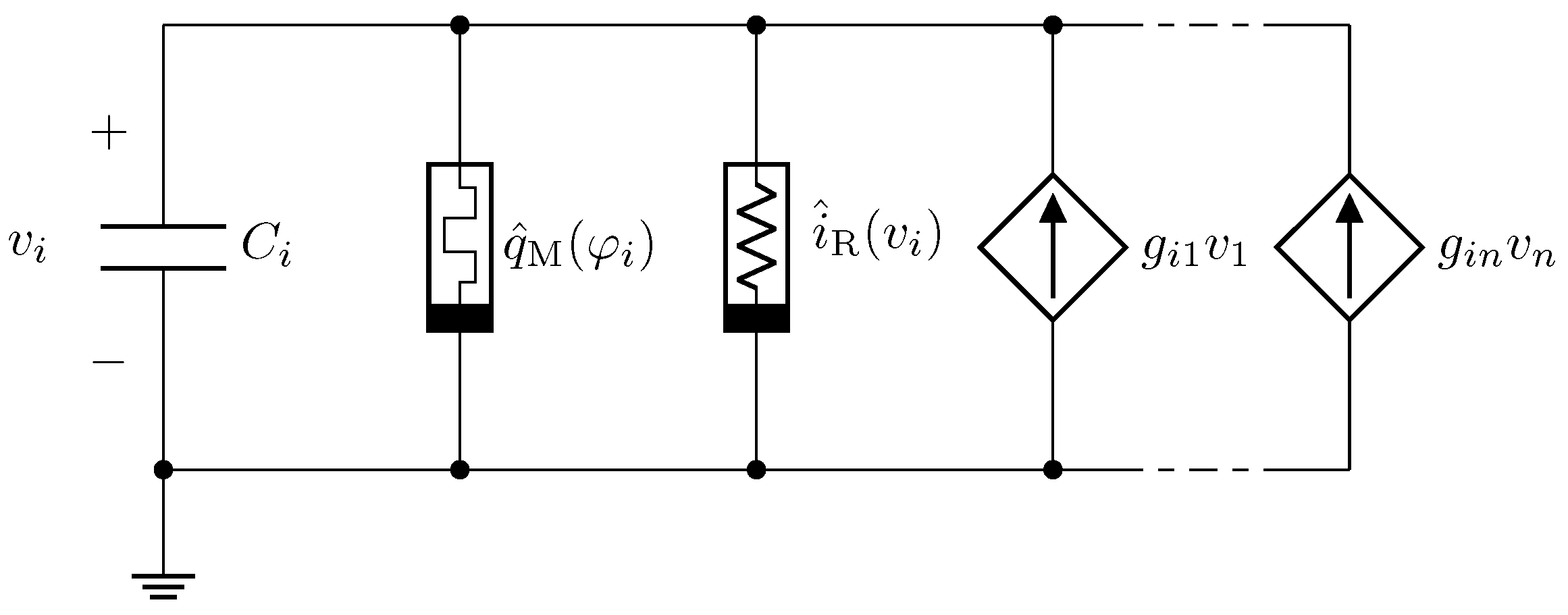
3.2. Real Memristor Neural Network Model

Ideal memristors are generally not well suited for modeling real memristive devices in nanotechnology. In this paper, this leads us to consider a real memristor neural network (RMNN) in which the ideal memristor in Figure 3 is replaced by a real extended memristor model that is similar to that discussed in Section 2. A schematic of an RMNN cell is depicted in Figure 4.

An RMNN satisfies the following system of differential equations:

$$\begin{array}{cc}\hfill C{\dot{v}}_i& =-{\widehat{q}}_{\mathrm{M}}^{\prime }({\phi }_i)v_i+\sum _{j=1}^n{g}_{ij}{v}_j-{\widehat{i}}_{\mathrm{R}}(v_i)\hfill \\ \hfill {\dot{\phi }}_i& =v_i\hfill \end{array}$$

(6)

for $i=1,\dots ,n$. In vector form, we have

$$\begin{array}{cc}\hfill C\dot{v}& =-{\widehat{Q}}_{\mathrm{M}}^{\prime }(\phi )v+Gv-{\widehat{I}}_{\mathrm{R}}(v)\hfill \\ \hfill \dot{\phi }& =v\hfill \end{array}$$

(7)

where ${\widehat{I}}_{\mathrm{R}}(v)={({\widehat{i}}_{\mathrm{R}}(v_1),\dots ,{\widehat{i}}_{\mathrm{R}}(v_n))}^{\top }\in {\mathbb{R}}^n$, which is an autonomous system of $2n$ differential equations in the state variables $(v,\phi )\in {\mathbb{R}}^{2n}$.

In this manuscript, we assume, unless stated otherwise, that the nonlinear resistor characteristic ${\widehat{i}}_{\mathrm{R}}$ satisfies Assumption 1. If, instead, ${\widehat{i}}_{\mathrm{R}}$ satisfies Assumption 2, we are brought back to the previous case by considering the system

$$\begin{array}{cc}\hfill C{\dot{v}}_i& =-{\widehat{q}}_{\mathrm{M}}^{\prime }({\phi }_i)v_i+(g_{ii}-\gamma )v_i+\sum _{j=1,\dots ,n;j\ne i}{g}_{ij}{v}_j-{\widehat{i}}_{\mathrm{R}}^{+}(v_i)\hfill \\ \hfill {\dot{\phi }}_i& =v_i\hfill \end{array}$$

(8)

for $i=1,\dots ,n$, where ${\widehat{i}}_{\mathrm{R}}^{+}$ now satisfies Assumption 1.

The equilibrium points (EPs) of (7) are obtained by letting $\dot{v}=0$ and $\dot{\phi }=0$. It is seen that for any $\overline{\phi }\in {\mathbb{R}}^n$, $(0,\overline{\phi })\in {\mathbb{R}}^{2n}$ is an EP. This means that (7) has an n-dimensional plane of EPs such that the voltages vanish at any EP.

4. Invariants of Motion and Lyapunov Functions

In this section, we establish some basic facts that will be used in the dynamic analysis of the paper.

Let us first consider the IMNN (5) and define the following n functions $Q_i:{\mathbb{R}}^{2n}\to \mathbb{R}$ of the state variables $(v,\phi )\in {\mathbb{R}}^{2n}$:

$$Q_i(v,\phi )\doteq C{v}_i+{\widehat{q}}_{\mathrm{M}}({\phi }_i)-\sum _{j=1}^n{g}_{ij}{\phi }_j$$

(9)

for $i=1,\dots ,n$.

Property 1.

Along the solutions of the IMNN (5), we have

$${\dot{Q}}_i(v,\phi )=0$$

for any t and any $i=1,\dots ,n$.

Proof. 

Since $v_i={\dot{\phi }}_i$, we have ${\widehat{q}}_{\mathrm{M}}^{\prime }({\phi }_i)v_i=\frac{d}{dt}{\widehat{q}}_{\mathrm{M}}({\phi }_i)$. Therefore, we can rewrite the IMNN equations as

$$\frac{d}{dt}\left(C{v}_i+{\widehat{q}}_{\mathrm{M}}({\phi }_i)-\sum _{j=1}^n{g}_{ij}{\phi }_j\right)=0$$

(10)

for any t and any $i=1,\dots ,n$. □

Property 1 means that the functions $Q_i$ are n invariants of motion for the IMNN (5). The existence of invariants of motion for the IMNN can be predicted on the basis of the flux–charge analysis method in [44]. However, their explicit expressions were not given in previous papers [32,35].

Let us now consider the RMNN (7). Now, due to the presence of nonlinear resistors ${\widehat{i}}_{\mathrm{R}}$ in the neuron cells, $Q_i$ are no longer invariants of motion. However, the following holds.

Property 2.

Suppose that ${\widehat{i}}_{\mathrm{R}}$ satisfies Assumption 1. Then, along the solutions of the RMNN (7), we have

$${\dot{Q}}_i(v,\phi )=-{\widehat{i}}_{\mathrm{R}}(v_i)\le 0$$

for any t and any $i=1,\dots ,n$.

Proof. 

We can rewrite the RMNN equations as

$$\frac{d}{dt}\left(C{v}_i+{\widehat{q}}_{\mathrm{M}}({\phi }_i)-\sum _{j=1}^n{g}_{ij}{\phi }_j\right)=-{\widehat{i}}_{\mathrm{R}}(v_i)$$

(11)

for any t and any $i=1,\dots ,n$. The result follows, since, according to Assumption 1, we have ${\widehat{i}}_{\mathrm{R}}(v_i)\ge 0$. □

Of course, an analogous result holds if ${\widehat{i}}_{\mathrm{R}}$ satisfies Assumption 2. Property 2 shows that if ${\widehat{i}}_{\mathrm{R}}$ satisfies either Assumption 1 or Assumption 2, then $Q_i$ are n Lyapunov functions that decrease along the solutions of the RMNN.

5. RMNNs in the Flux–Charge Domain

In this section, we provide two equivalent representations of the RMNN (7) in the integral variables of flux and charge (cf. Section 2), which will be useful in analyzing the convergence of the solutions and for the numerical verification.

We denote by $(v(t;v_0,{\phi }_0),\phi (t;v_0,{\phi }_0))$ the solution of the RMNN (7) with initial conditions (ICs) $(v_0,{\phi }_0)\in {\mathbb{R}}^{2n}$ at $t=0$ and assume that it is defined for $t\ge 0$. Under Assumption 1, due to Property 2, we have

$$\frac{d}{dt}{Q}_i(v(t;v_0,{\phi }_0),\phi (t;v_0,{\phi }_0))=-{\widehat{i}}_{\mathrm{R}}(v_i(t;v_0,{\phi }_0))\le 0$$

for any t and any $i=1,\dots ,n$; so,

$$Q_i(v(t;v_0,{\phi }_0),\phi (t;v_0,{\phi }_0))-Q_i(v_0,{\phi }_0)=-q_{\mathrm{R},i}(t;v_0,{\phi }_0)\le 0$$

(12)

where

$$q_{\mathrm{R},i}(t;v_0,{\phi }_0)\doteq {\int }_0^t{\widehat{i}}_{\mathrm{R}}(v_i(\sigma ;v_0,{\phi }_0))d\sigma .$$

(13)

Note that since $i_{\mathrm{R},i}\ge 0$, $-q_{\mathrm{R},i}$ is a monotonically decreasing function of time.

Let us now consider the system of differential equations

$$\begin{array}{cc}\hfill C{\dot{\varphi }}_i& =-{\widehat{q}}_{\mathrm{M}}({\varphi }_i)+\sum _{j=1}^n{g}_{ij}{\varphi }_j+Q_i(v_0,{\phi }_0)-q_{\mathrm{R},i}(t;v_0,{\phi }_0)\hfill \\ \hfill & =-{\widehat{q}}_{\mathrm{M}}({\varphi }_i)+\sum _{j=1}^n{g}_{ij}{\varphi }_j+Q_i(v(t;v_0,{\phi }_0),{\phi }_i(t;v_0,{\phi }_0))\hfill \end{array}$$

(14)

for $i=1,\dots ,n$. In vector form, we have

$$\begin{array}{cc}\hfill C\dot{\varphi }& =-{\widehat{Q}}_{\mathrm{M}}(\varphi )+G\varphi +Q(v_0,{\phi }_0)-Q_{\mathrm{R}}(t;v_0,{\phi }_0)\hfill \\ \hfill & =-{\widehat{Q}}_{\mathrm{M}}(\varphi )+G\varphi +Q(v(t;v_0,{\phi }_0),\phi (t;v_0,{\phi }_0))\hfill \end{array}$$

(15)

where $\varphi ={({\varphi }_1,\dots ,{\varphi }_n)}^{\top }\in {\mathbb{R}}^n$ and $Q_{\mathrm{R}}(t;v_0,{\phi }_0)={(q_{\mathrm{R},1}(t;v_0,{\phi }_0),\dots ,q_{\mathrm{R},n}(t;v_0,{\phi }_0))}^{\top }\in {\mathbb{R}}^n$. Note that (15) is a non-autonomous system of n differential equations in the state variables $\varphi \in {\mathbb{R}}^n$ and that the time-dependent forcing term $-Q_{\mathrm{R}}$ depends on $v_0$ and ${\phi }_0$.

We denote by $\varphi (t;{\phi }_0)$ the solution of (15) with IC ${\phi }_0\in {\mathbb{R}}^n$ at $t=0$ and assume that it is defined for $t\ge 0$. The next result gives a link between the solutions of (15) and (7).

Property 3.

We have

$$\varphi (t;{\phi }_0)=\phi (t;v_0,{\phi }_0)$$

and, conversely,

$$(v(t;v_0,{\phi }_0),\phi (t;v_0,{\phi }_0))=(\dot{\varphi }(t;{\phi }_0),\varphi (t;{\phi }_0))$$

for any $t\ge 0$.

Proof. 

Integrating both sides of the first equation of (7), we get

$$\begin{array}{cc}\hfill C\dot{\phi }-C{v}_0=& -{\widehat{Q}}_{\mathrm{M}}(\phi )+{\widehat{Q}}_{\mathrm{M}}({\phi }_0)+G\phi -G{\phi }_0-{\int }_0^t{\widehat{I}}_{\mathrm{R}}(v(\sigma ;v_0,{\phi }_0))d\sigma \hfill \end{array}$$

where we consider that

$${\int }_0^t{\widehat{Q}}_{\mathrm{M}}^{\prime }(\phi (\sigma ))v(\sigma )d\sigma ={\int }_{{\phi }_0}^{\phi (t)}{\widehat{Q}}_{\mathrm{M}}(\theta )d\theta ={\widehat{Q}}_{\mathrm{M}}(\phi (t))-{\widehat{Q}}_{\mathrm{M}}({\phi }_0)$$

and $v=\dot{\phi }$. Taking (9) into account, we have $Q(v_0,{\phi }_0)=C{v}_0+{\widehat{Q}}_{\mathrm{M}}({\phi }_0)-G{\phi }_0$; hence,

$$C\dot{\phi }=-{\widehat{Q}}_{\mathrm{M}}(\phi )+G\phi +Q(v_0,{\phi }_0)-Q_{\mathrm{R}}(t;v_0,{\phi }_0).$$

Let $(v(t;v_0,{\phi }_0),\phi (t;v_0,{\phi }_0))$ be the solution of (7) with ICs $(v_0,{\phi }_0)\in {\mathbb{R}}^{2n}$. Due to the uniqueness of the solution to a Cauchy problem, it can be easily checked that $\phi (t;v_0,{\phi }_0)$ is also the solution of (15) with the IC ${\phi }_0$, i.e., $\varphi (t;{\phi }_0)=\phi (t;v_0,{\phi }_0)$.

Differentiating both sides of (15), denoting $w=\dot{\varphi }$, and taking (13) into account, we obtain

$$\begin{array}{cc}\hfill C\dot{w}=& -{\widehat{Q}}_{\mathrm{M}}^{\prime }(\varphi )w+Gw-{\widehat{I}}_{\mathrm{R}}(w)\hfill \\ \hfill \dot{\varphi }=& w.\hfill \end{array}$$

Now, let $\varphi (t;{\phi }_0)$ be the solution of (15) with the IC ${\phi }_0\in {\mathbb{R}}^n$. Then, $(\dot{\varphi }(t;{\phi }_0),\varphi (t;{\phi }_0))$ is the solution of (7) with the ICs $(\dot{\varphi }(0,{\phi }_0),{\phi }_0)$. From (14), we have $C\dot{\varphi }(0;{\phi }_0)=-{\widehat{Q}}_{\mathrm{M}}(\varphi (0;{\phi }_0))$ + $G\varphi (0;{\phi }_0)+Q(v_0,{\phi }_0)$ and, since $\varphi (0,{\phi }_0)={\phi }_0$ and $Q(v_0,{\phi }_0)=C{v}_0+{\widehat{Q}}_{\mathrm{M}}({\phi }_0)-G{\phi }_0$, we obtain $\dot{\phi }(0;{\phi }_0)=v_0$. Therefore, we have verified that $(v(t;v_0,{\phi }_0),\phi (t;v_0,{\phi }_0))=(\dot{\varphi }(t;{\phi }_0),\varphi (t;{\phi }_0)).$ □

Consider now

$$\begin{array}{cc}\hfill C\dot{\psi }& =-{\widehat{Q}}_{\mathrm{M}}(\psi )+G\psi +Q(v_0,{\phi }_0)-{\mathcal{Q}}_{\mathrm{R}}\hfill \\ \hfill {\dot{\mathcal{Q}}}_{\mathrm{R}}& ={\widehat{I}}_{\mathrm{R}}\left(\frac{1}{C}(-{\widehat{Q}}_{\mathrm{M}}(\psi )+G\psi +Q(v_0,{\phi }_0)-{\mathcal{Q}}_{\mathrm{R}})\right)\hfill \end{array}$$

(16)

where $\psi ,{\mathcal{Q}}_{\mathrm{R}}\in {\mathbb{R}}^n$. This is an autonomous system of $2n$ differential equations in the state variables $(\psi ,{\mathcal{Q}}_{\mathrm{R}})\in {\mathbb{R}}^{2n}$.

Let $(\psi (t;{\phi }_0,0),{\mathcal{Q}}_{\mathrm{R}}(t;{\phi }_0,0))$ denote the solution of (16) with ICs $({\phi }_0,0)\in {\mathbb{R}}^{2n}$. The next results establish links between the solutions of (16) and (15) and those of (16) and (7).

Property 4.

We have

$$(\psi (t;{\phi }_0,0),{\mathcal{Q}}_{\mathrm{R}}(t;{\phi }_0,0))=(\varphi (t;{\phi }_0),{\int }_0^t{\widehat{I}}_{\mathrm{R}}(\dot{\varphi }(\sigma ;{\phi }_0))d\sigma )$$

and, conversely,

$$\varphi (t;{\phi }_0)=\psi (t;{\phi }_0,0)$$

for any $t\ge 0$.

Proof. 

Let $\varphi (t;{\phi }_0)$ be the solution of (15) with the IC ${\phi }_0$ at $t=0$. We have

$$\begin{array}{c}\hfill \dot{\varphi }=\frac{1}{C}({\widehat{Q}}_{\mathrm{M}}(\varphi )+G\varphi +Q(v_0,{\phi }_0)-Q_{\mathrm{R}}(t;v_0,{\phi }_0)).\end{array}$$

(17)

Due to Property 3, $v(t;v_0,{\phi }_0)=\dot{\varphi }(t;{\phi }_0)$. Differentiating both sides of (13), we obtain ${\dot{Q}}_{\mathrm{R}}(·;v_0,{\phi }_0))={\widehat{I}}_{\mathrm{R}}(\dot{\varphi }(·;{\phi }_0)).$ Taking into account (17) and Property 3, we obtain the Cauchy problem:

$$\begin{array}{cc}\hfill C\dot{\varphi }=& -{\widehat{Q}}_{\mathrm{M}}(\varphi )+G\varphi +Q(v_0,{\phi }_0)-Q_{\mathrm{R}}\hfill \\ \hfill {\dot{Q}}_{\mathrm{R}}=& {\widehat{I}}_{\mathrm{R}}\left(\frac{1}{C}({\widehat{Q}}_{\mathrm{M}}(\varphi )+G\varphi +Q(v_0,{\phi }_0)-Q_{\mathrm{R}})\right)\hfill \end{array}$$

with the IC $({\phi }_0,0)$. As a consequence, $(\varphi (t;v_0),{\int }_0^t{\widehat{I}}_{\mathrm{R}}(\dot{\varphi }(\sigma ;{\phi }_0))d\sigma )$ is the solution of (16) with the IC $({\phi }_0,0)$.

Now, let $(\psi (t;{\phi }_0,0),{\mathcal{Q}}_{\mathrm{R}}(t;{\phi }_0,0))$ be the solution of (16) with the ICs $({\phi }_0,0)$. By noting that ${\mathcal{Q}}_{\mathrm{R}}(t;{\phi }_0,0)=0$, taking (13) into account, we can rewrite the first equation of (16) as

$$\dot{\psi }=-{\widehat{Q}}_{\mathrm{M}}(\psi )+G\psi +Q(v_0,{\phi }_0)-{\int }_0^t{\widehat{I}}_{\mathrm{R}}(\dot{\psi }(\sigma ;{\phi }_0,0))d\sigma .$$

As a consequence, $\psi (t;{\phi }_0,0)$ is also a solution of (15) with the IC ${\phi }_0$. □

Property 5.

We have

$$(\psi (t;{\phi }_0,0),{\mathcal{Q}}_{\mathrm{R}}(t;{\phi }_0,0))=(\phi (t;v_0,{\phi }_0),{\int }_0^t{\widehat{I}}_{\mathrm{R}}(v(\sigma ;v_0,{\phi }_0))d\sigma )$$

and, conversely,

$$(v(t;v_0,{\phi }_0),\phi (t;v_0,{\phi }_0))=(\dot{\psi }(t;{\phi }_0,0),\psi (t;{\phi }_0,0))$$

for any $t\ge 0$.

Proof. 

The result is a straightforward consequence of Properties 3 and 4. □

6. Main Results on the Convergence of RMNNs

Suppose that Assumption 1 is satisfied and consider a solution $(v(t;v_0,{\phi }_0),\phi (t;v_0,{\phi }_0))$ of the RMNN (7) that is defined for $t\ge 0$. Since $-q_{\mathrm{R},i}$ in (13) is monotonically non-increasing, for any $i=1,\dots ,n$, we have that either $-q_{\mathrm{R},i}(t;v_0,\phi )\to -\infty$ as $t\to \infty$ or $-q_{\mathrm{R},i}(t;v_0,\phi )\to -q_{\mathrm{R},i}^{\infty }(v_0,{\phi }_0)>-\infty$ as $t\to \infty$.

Property 6.

If the solution $(v(t;v_0,{\phi }_0),\phi (t;v_0,{\phi }_0))$ of the RMNN (7) is defined and bounded for $t\ge 0$, then we have

$$\underset{t\to \infty }{lim}(-q_{\mathrm{R},i}(t;v_0,\phi ))=-q_{\mathrm{R},i}^{\infty }(v_0,{\phi }_0)>-\infty$$

for $i=1,\dots ,n$.

Proof. 

From Properties 3–5, $\phi (t;v_0,{\phi }_0)=\varphi (t;{\phi }_0)=\psi (t;{\phi }_0,0)$ and $v(t;v_0,{\phi }_0)$ = $\dot{\phi }(t;v_0,{\phi }_0)=\dot{\varphi }(t;{\phi }_0)=\dot{\psi }(t;{\phi }_0,0)$. Additionally, $Q_{\mathrm{R}}(t;v_0,{\phi }_0)={\mathcal{Q}}_{\mathrm{R}}(t;{\phi }_0,0)$. Now, consider (16). Since $(v(t;v_0,{\phi }_0),\phi (t;v_0,{\phi }_0))$ is bounded for $t\ge 0$, and $\psi (t;{\phi }_0,0),$$\dot{\psi }(t;{\phi }_0,0),$${\widehat{Q}}_{\mathrm{R}}(\psi (t;{\phi }_0,0))$, and $G\psi (t;{\phi }_0,0)$ are bounded for $t\ge 0$; this implies that ${\mathcal{Q}}_{\mathrm{R}}(t;{\phi }_0,0)$ and $Q(t;v_0,{\phi }_0)$ are bounded for $t\ge 0$. Since $Q(t;v_0,{\phi }_0)$ is monotonically non-increasing for $t\ge 0$, there exists $Q_{\mathrm{R}}^{\infty }(v_0,{\phi }_0)>-\infty$ such that ${lim}_{t\to \infty }{Q}_{\mathrm{R}}(t;v_0,{\phi }_0)=Q_{\mathrm{R}}^{\infty }(v_0,{\phi }_0)$. □

Under the assumptions of Property 6, we can consider the following asymptotic system in the flux–charge domain:

$$\begin{array}{cc}\hfill C\dot{\Phi }& =-{\widehat{Q}}_{\mathrm{M}}(\Phi )+G\Phi +Q_0(v_0,{\phi }_0)-Q_{\mathrm{R}}^{\infty }(v_0,{\phi }_0)\hfill \\ \hfill & =-{\widehat{Q}}_{\mathrm{M}}(\Phi )+G\Phi +Q^{\infty }(v_0,{\phi }_0)\hfill \end{array}$$

(18)

where

$$Q_{\mathrm{R}}^{\infty }(v_0,{\phi }_0)={(q_{\mathrm{R},1}^{\infty }(v_0,{\phi }_0),\dots ,q_{\mathrm{R},n}^{\infty }(v_0,{\phi }_0))}^{\top }={\int }_0^{\infty }{\widehat{I}}_{\mathrm{R}}(v(\sigma ;v_0,{\phi }_0))d\sigma \in {\mathbb{R}}^n$$

and $Q^{\infty }(v_0,{\phi }_0)={lim}_{t\to \infty }Q(t;v_0,{\phi }_0)\in {\mathbb{R}}^n$.

The next theorem gives the main convergence result in the paper.

Theorem 1.

Assume for the RMNN that the interconnection matrix G is symmetric. In addition, suppose that the solution $(v(t;v_0,{\phi }_0),\phi (t;v_0,{\phi }_0))$ of the RMNN (7) is defined and bounded for $t\ge 0$ and that the EPs of the asymptotic system (18) are isolated. Then:

(1) 

$\varphi (t;{\phi }_0)$ converges to $\eta \in {\mathbb{R}}^n$ as $t\to \infty$, where η is an EP of (18);

(2) 

$(v(t;v_0,{\phi }_0),\phi (t;v_0,{\phi }_0))$ converges to the EP $(0,\eta )\in {\mathbb{R}}^{2n}$ of (7) as $t\to \infty$;

(3) 

$(\psi (t;{\phi }_0,0),{\mathcal{Q}}_{\mathrm{R}}(t;{\phi }_0,0))$ converges to the EP $(\eta ,Q_{\mathrm{R}}^{\infty }(v_0,{\phi }_0))$ of (16) as $t\to \infty$.

We provide some remarks before giving the proof of the theorem.

• Theorem 1 can be considered an extension of the convergence results obtained in [32] for IMNNs to NNs with real memristors. Basically, Theorem 1 states that the presence of rectifying nonlinear resistors in the neuron model does not destroy the property of convergence that holds for symmetric IMNNs.
• It is worth remarking that the assumption of isolated EPs for the asymptotic system (18) is not restrictive. Indeed, in the case in which the system has non-isolated EPs, the vector field defining (18) can be changed by an arbitrarily small amount to obtain isolated EPs. This can be shown via an argument based on the Sard theorem analogous to that used to prove ([32], Property 2) (details are omitted).
• The convergence result in Theorem 1 has been proven via a Lyapunov approach applied to the system describing the RMNN in the flux–charge (integral) domain. A crucial property is that the functions $Q_i$, $i=1,\dots ,n$, in (9) can be used as Lyapunov functions that decrease along the RMNN equations in the voltage–current domain. This enables an association of an asymptotic system in the flux–charge domain—to which the Lyapunov approach can be effectively used to prove convergence—with an RMNN.
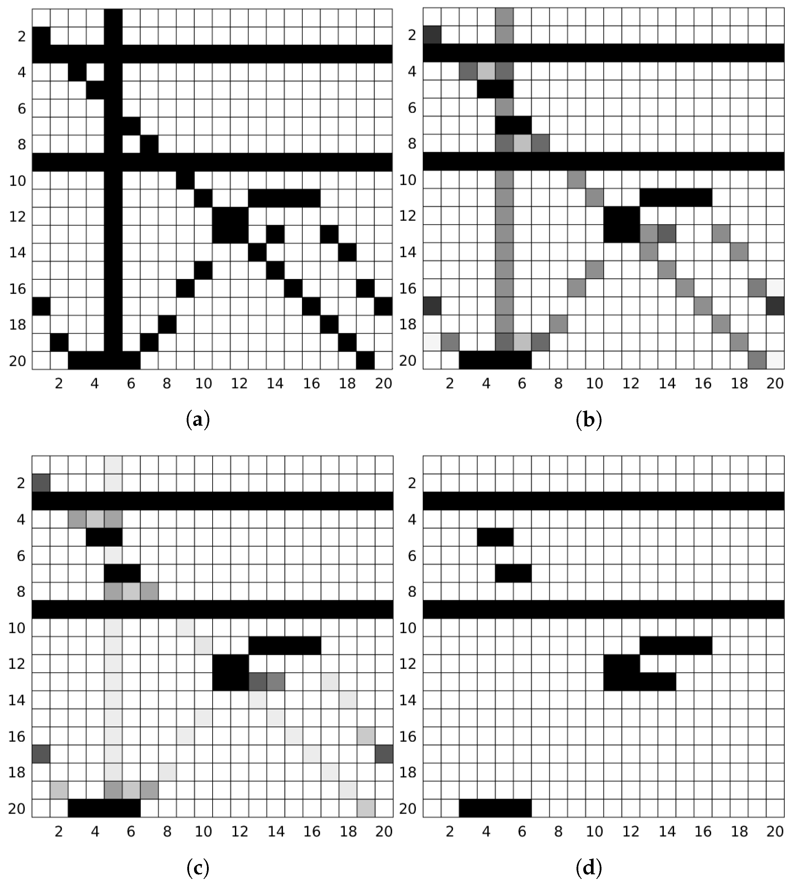
• From an the point of view of applications, an RMNN can be used to process signals and images in the flux–charge domain, i.e., the dynamics of the memristor fluxes can be used instead of using the dynamics of capacitor voltages, as happens for traditional memristor-less NNs operating in the voltage–current domain. A simple application to an image processing task will be illustrated in Section 7. We stress that in an RMNN, memristors are used in the analog computation, but they are also able to store the computational result, i.e., the asymptotic values of fluxes, in accordance with the principle of in-memory computing.

Proof of Theorem 1.

(1) Suppose, for simplicity, that $C=1$. Let us consider for (15) the candidate Lyapunov function

$$E(\varphi )=\sum _{i=1}^n{\int }_0^{{\varphi }_i}{\widehat{q}}_{\mathrm{M}}(\sigma )d\sigma -\frac{1}{2}{\varphi }^{\top }G\varphi -{\varphi }^{\top }(Q_0(v_0,{\phi }_0)-Q_{\mathrm{R}}^{\infty }(v_0,{\phi }_0))$$

where $Q_{\mathrm{R}}^{\infty }(v_0,{\phi }_0)$ is defined in Property 6. Since, by assumption, $\phi (t;v_0,{\phi }_0)$ is bounded for $t\ge 0$, due to Property 3, we have that $\varphi (t;{\phi }_0)$ is bounded for $t\ge 0$ and, since E is continuous, $E(\varphi (t;v_0))$ is bounded from below for $t\ge 0$.

Accounting for the symmetry of G, we have

$$\begin{array}{cc}\hfill \nabla E(\varphi )=& {\widehat{Q}}_{\mathrm{M}}(\varphi )-G\varphi -Q(v_0,{\phi }_0)+Q_{\mathrm{R}}^{\infty }(v_0,{\phi }_0).\hfill \end{array}$$

(19)

Hence, (15) can be written as

$$\dot{\varphi }=-\nabla E(\varphi )-Q_{\mathrm{R}}(t;v_0,{\phi }_0)+Q_{\mathrm{R}}^{\infty }(v_0,{\phi }_0)$$

(20)

while the asymptotic system (18) is

$$\dot{\Phi }=-\nabla E(\Phi ).$$

(21)

Then, the time derivative of E along the solutions of (20) is given by

$$\begin{array}{cc}\hfill \dot{E}(\varphi )& =\nabla E{(\varphi )}^{\top }(-\nabla E(\varphi )-Q_{\mathrm{R}}(t;v_0,{\phi }_0)+Q_{\mathrm{R}}^{\infty }(v_0,{\phi }_0))\hfill \\ \hfill & =-{\parallel \nabla E(\varphi )\parallel }^2-\nabla E{(\varphi )}^{\top }(Q_{\mathrm{R}}(t;v_0,{\phi }_0)-Q_{\mathrm{R}}^{\infty }(v_0,{\phi }_0)).\hfill \end{array}$$

(22)

We choose $r>0$ such that $\varphi (t;{\varphi }_0)\in B(0,r)$ for any $t\ge 0$. Let us first show that (21) has at least an EP in $\overline{B(0,R)}$, where $R>r$. The EPs of (21) are the points where $\nabla E=0$. Suppose, for contradiction, that (21) has no EPs in $\overline{B(0,r)}$. Since $\nabla E$ is continuous and $\nabla E\ne 0$, then $-{\parallel \nabla E(\Phi )\parallel }^2\le -m^2<0$ for any $\Phi \in \overline{B(0,r)}$. Moreover, $\parallel \nabla E(\Phi )\parallel \le M$ if $\Phi \in \overline{B(0,r)}$. Since $Q_{\mathrm{R}}(t;v_0,{\phi }_0)$ is monotonically non-increasing for $t\ge 0$ and it tends towards $Q_{\mathrm{R}}^{\infty }(v_0,{\phi }_0)$ as $t\to \infty$, there exists $\overline{t}$ such that $\parallel Q_{\mathrm{R}}(t;v_0,{\phi }_0)-Q_R^{\infty }(v_0,{\phi }_0))\parallel <m^2/(2M)$ for any $t\ge \overline{t}$. Then, for $t\ge \overline{t}$, $\dot{E}(\varphi (t;{\phi }_0))\le -\parallel \nabla E(\varphi (t;{\phi }_0)){\parallel }^2+\parallel \nabla E(\varphi (t;{\phi }_0))\parallel \parallel Q_R(t;v_0,{\phi }_0)-Q_R^{\infty }(v_0,{\phi }_0)\parallel <-m^2/2<0$. Therefore, $E(\varphi (t;{\phi }_0))\to -\infty$ as $t\to \infty$, which is a contradiction.

Since the EPs of (18) are isolated, it follows that there exist finite EPs ${\eta }_1,\dots ,{\eta }_p$ of (18) in $B(0,R)$. We choose $\overline{ϵ}>0$ such that $B({\eta }_i,\overline{ϵ})\subset B(0,R)$ and $B({\eta }_i,\overline{ϵ})\cap B({\eta }_j,\overline{ϵ})=\varnothing$ for any $i,j=1,\dots ,p$. We want to prove that there exists $\overline{i}\in \{1,\dots ,p\}$ such that for any $0<ϵ\le \overline{ϵ}$, there exists $t_{ϵ}\ge 0$ such that $\varphi (t;{\phi }_0)\in B({\eta }_{\overline{i}},ϵ)$ for any $t\ge t_{ϵ}$. This, in turn, implies the convergence of $\varphi (·;{\phi }_0)$ to the EP ${\eta }_{\overline{i}}$.

For any $\lambda >0$, we let

$${\mathcal{I}}_{\lambda }={\cup }_{i=1}^{p}B({\eta }_i,\lambda )\subset B(0,R)$$

and

$${\mathcal{O}}_{\lambda }=B(0,R)\setminus {\mathcal{I}}_{\lambda }.$$

Let us show the next preliminary property.

Property 7.

Suppose that the assumptions of Theorem 1 are satisfied. Then, for any $0<\lambda <\overline{ϵ}$, the following hold:

(a) There exist ${\alpha }^2(\lambda )>0$ and $t_{\lambda }\ge 0$ such that for $t\ge t_{\lambda }$, we have

$$\dot{E}(\varphi )\le -{\alpha }^2(\lambda )<0$$

if $\varphi \in \overline{{\mathcal{O}}_{\lambda }}$;

(b) we have

$$\underset{\varphi \in \overline{{\mathcal{I}}_{\lambda }}}{max}E(\varphi )-\underset{\varphi \in \overline{{\mathcal{I}}_{\lambda }}}{min}E(\varphi )\le {\beta }^2(\lambda )$$

where ${\beta }^2(\lambda )\to 0$ as $\lambda \to 0$.

Proof. 

(a) Since $\nabla E$ is continuous and there is no EP of (18) in $\overline{{\mathcal{O}}_{\lambda }}$, there exists ${\alpha }^2(\lambda )>0$ such that $-{\parallel \nabla E(\varphi )\parallel }^2\le -2{\alpha }^2(\lambda )<0$ if $\varphi \in \overline{{\mathcal{O}}_{\lambda }}$. Taking into account (19), we have, for any $\varphi \in \overline{{\mathcal{O}}_{\lambda }}$,

$$\parallel \nabla E(\varphi )\parallel \le {\widehat{M}}_{\lambda }+R\parallel G\parallel +\parallel Q(v_0,{\phi }_0)\parallel +\parallel Q_{\mathrm{R}}^{\infty }(v_0,{\phi }_0)\parallel$$

where ${\widehat{M}}_{\lambda }={max}_{\varphi \in \overline{{\mathcal{O}}_{\lambda }}}{\widehat{Q}}_{\mathrm{M}}(\varphi )<\infty$. Since $Q_R(t;v_0,{\phi }_0)$ is monotonically non-increasing for $t\ge 0$ and it tends towards $Q_R^{\infty }(v_0,{\phi }_0)$ as $t\to \infty$, there exists $t_{\lambda }$ such that

$$\parallel Q_R(t;v_0,{\phi }_0)-Q_R^{\infty }(v_0,{\phi }_0))\parallel <{\alpha }^2(\lambda )/({\widehat{M}}_{\lambda }+R\parallel G\parallel +\parallel Q(v_0,{\phi }_0)\parallel +\parallel Q_{\mathrm{R}}^{\infty }(v_0,{\phi }_0)\parallel )$$

for any $t\ge t_{\lambda }$. Then, taking (22) into account, we obtain

$$\dot{E}(\varphi )\le -{\parallel \nabla E(\varphi )\parallel }^2+\parallel \nabla E(\varphi )\parallel \parallel Q_R(t;v_0,{\phi }_0)-Q_R^{\infty }(v_0,{\phi }_0)\parallel <-{\alpha }^2(\lambda )<0$$

for all $t\ge t_{\lambda }$.

(b) Since $\varphi \in \overline{{\mathcal{I}}_{\lambda }}$, there exists $\overline{j}\in \{1,\dots ,p\}$ such that $\varphi ={\eta }_{\overline{j}}+{\Delta }_{\overline{j}}$, with ${\Delta }_{\overline{j}}\in B(0,\lambda )$. We can write $E(\varphi )$ as

$$\begin{array}{cc}\hfill E({\eta }_{\overline{j}}+{\Delta }_{\overline{j}})& =\sum _{i=1}^n{\int }_0^{{\eta }_{\overline{j},i}+{\Delta }_{\overline{j},i}}{\widehat{q}}_{\mathrm{M}}(\sigma )d\sigma -\frac{1}{2}{({\eta }_{\overline{j}}+{\Delta }_{\overline{j}})}^{\top }G({\eta }_{\overline{j}}+{\Delta }_{\overline{j}})\hfill \\ \hfill & -{({\eta }_{\overline{j}}+{\Delta }_{\overline{j}})}^{\top }(Q_0(v_0,{\phi }_0)-Q_{\mathrm{R}}^{\infty }(v_0,{\phi }_0)).\hfill \end{array}$$

The following inequalities hold true:

$$\begin{array}{cc}\hfill \underset{{\Delta }_{\overline{j}}\in \overline{B(0,\lambda )}}{max}E({\eta }_{\overline{j}}+{\Delta }_{\overline{j}})\le & \sum _{i=1}^n{\int }_0^{{\eta }_{\overline{j},i}}{\widehat{q}}_{\mathrm{M}}(\sigma )d\sigma +\lambda \sum _{i=1}^n\underset{\sigma \in [{\eta }_{\overline{j},i}-\lambda ,{\eta }_{\overline{j},i}+\lambda ]}{max}|{\widehat{q}}_{\mathrm{M}}(\sigma )|\hfill \\ \hfill & -\frac{1}{2}{\eta }_{\overline{j}}^{\top }G{\eta }_{\overline{j}}+\rho (G)\lambda \parallel {\eta }_{\overline{j}}\parallel +\frac{1}{2}\rho (G){\lambda }^2\hfill \\ \hfill & -{\eta }_{\overline{j}}^{\top }(Q_0(v_0,{\phi }_0)-Q_{\mathrm{R}}^{\infty }(v_0,{\phi }_0))+\lambda \parallel Q_0(v_0,{\phi }_0)-Q_{\mathrm{R}}^{\infty }(v_0,{\phi }_0)\parallel \hfill \end{array}$$

and

$$\begin{array}{cc}\hfill \underset{{\Delta }_{\overline{j}}\in \overline{B(0,\lambda )}}{min}E({\eta }_{\overline{j}}+{\Delta }_{\overline{j}})\ge & \sum _{i=1}^n{\int }_0^{{\eta }_{\overline{j},i}}{\widehat{q}}_{\mathrm{M}}(\sigma )d\sigma -\lambda \sum _{i=1}^n\underset{\sigma \in [{\eta }_{\overline{j},i}-\lambda ,{\eta }_{\overline{j},i}+\lambda ]}{max}|{\widehat{q}}_{\mathrm{M}}(\sigma )|\hfill \\ \hfill & -\frac{1}{2}{\eta }_{\overline{j}}^{\top }G{\eta }_{\overline{j}}-\rho (G)\lambda \parallel {\eta }_{\overline{j}}\parallel -\frac{1}{2}\rho (G){\lambda }^2\hfill \\ \hfill & -{\eta }_{\overline{j}}^{\top }(Q_0(v_0,{\phi }_0)-Q_{\mathrm{R}}^{\infty }(v_0,{\phi }_0))-\lambda \parallel Q_0(v_0,{\phi }_0)-Q_{\mathrm{R}}^{\infty }(v_0,{\phi }_0)\parallel \hfill \end{array}$$

where $\rho (G)$ is the spectral radius of G. These imply that

$$\begin{array}{cc}\hfill & \underset{{\Delta }_{\overline{j}}\in \overline{B(0,\lambda )}}{max}E({\eta }_{\overline{j}}+{\Delta }_{\overline{j}})-\underset{{\Delta }_{\overline{j}}\in \overline{B(0,\lambda )}}{min}E({\eta }_{\overline{j}}+{\Delta }_{\overline{j}})\hfill \\ \hfill & \le \lambda \left(2\parallel {\eta }_{\overline{j}}\parallel \rho (G)+2\sum _{i=1}^n\underset{\sigma \in [{\eta }_{\overline{j},i}-\lambda ,{\eta }_{\overline{j},i}+\lambda ]}{max}|{\widehat{q}}_{\mathrm{M}}(\sigma )|\right)\hfill \\ \hfill & +\lambda \left(\rho (G)\lambda +2\parallel Q_0(v_0,{\phi }_0)-Q_{\mathrm{R}}^{\infty }(v_0,{\phi }_0)\parallel \right)\hfill \\ \hfill & \doteq {\beta }_{\overline{j}}^2(\lambda ).\hfill \end{array}$$

It can be easily checked that ${\beta }_{\overline{j}}^2(\lambda )\to 0$ as $\lambda \to 0$. To complete the proof, it suffices to pick

$$\begin{array}{cc}\hfill {\beta }^2(\lambda )& =2\lambda \underset{\overline{j}=1,\dots ,p}{max}\left(\rho (G)\parallel {\eta }_{\overline{j}}\parallel +\sum _{i=1}^n\underset{\sigma \in [{\eta }_{\overline{j},i}-\lambda ,{\eta }_{\overline{j},i}+\lambda ]}{max}|{\widehat{q}}_{\mathrm{M}}(\sigma )|\right)\hfill \\ \hfill & +\lambda \left(\rho (G)\lambda +2\parallel Q_0(v_0,{\phi }_0)-Q_{\mathrm{R}}^{\infty }(v_0,{\phi }_0)\parallel \right).\hfill \end{array}$$

 □

For any $i\in \{1,\dots ,p\}$, we consider $B({\eta }_i,ϵ)$, $B({\eta }_i,ϵ/2)$, and $B({\eta }_i,\rho )$, where $\rho \le ϵ/2$. Moreover, we consider the sets ${\mathcal{O}}_{ϵ/2}$ and ${\mathcal{O}}_{\rho }$. By applying Property 7 with $\lambda =ϵ/2$, we find that there exists $t_{ϵ/2}$ such that $t\ge t_{ϵ/2}$ implies $\dot{E}(\varphi )\le -{\alpha }^2(ϵ/2)<0$ if $\varphi \in \overline{{\mathcal{O}}_{ϵ/2}}$. In particular, this is true if $\varphi \in \overline{B({\eta }_i,ϵ)-B({\eta }_i,ϵ/2)}$ and $i=1,\dots ,p$. Since ${\beta }^2(\lambda )\to 0$ as $\lambda \to 0$, we can choose $\rho$ and $\delta >0$ such that

$$\frac{ϵ}{{\rm Y}}{\alpha }^2\left(\frac{ϵ}{2}\right)>{\beta }^2(\rho )+\delta$$

where we let

$$\begin{array}{cc}\hfill {\rm Y}& \doteq {\sup }_{\varphi \in \overline{B(0,R)},t\ge 0}\parallel \dot{\varphi }(t)\parallel \hfill \\ \hfill & \le \parallel \nabla E(\varphi )\parallel +2\parallel Q_{\mathrm{R}}^{\infty }(v_0,{\phi }_0)\parallel \hfill \\ \hfill & \le {\widehat{M}}_{ϵ/2}+\parallel G\parallel R+\parallel Q(v_0,{\phi }_0)\parallel +3\parallel Q_{\mathrm{R}}^{\infty }(v_0,{\phi }_0)\parallel \hfill \end{array}$$

where ${\widehat{M}}_{ϵ/2}={max}_{\varphi \in \overline{{\mathcal{O}}_{ϵ/2}}}\parallel {\widehat{Q}}_{\mathrm{M}}(\varphi )\parallel$. Due to Property 7, with $\lambda =\rho$, we have that there exists $t_{\rho }\ge 0$ such that for $t\ge t_{\rho }$, we have $\dot{E}(\varphi )\le -{\alpha }^2(\rho )<0$ if $\varphi \in \overline{{\mathcal{O}}_{\rho }}$. In particular, this is true if $\varphi \in \overline{B({\eta }_i,ϵ/2)-B({\eta }_i,\rho )}$ and $i=1,\dots ,n$.

We say that $\varphi (·,{\phi }_0)$ undergoes an input–output event if for some $i\in \{1,\dots ,p\}$, there exist $t_{\mathrm{in}}<t^{+}<t_{\mathrm{out}}$ such that $\varphi (t_{\mathrm{in}},{\phi }_0)\in \partial B({\eta }_i,ϵ)$, $\varphi (t^{+},{\phi }_0)\in B({\eta }_i,\rho )$, and $\varphi (t_{\mathrm{out}},{\phi }_0)\in \partial B({\eta }_i,ϵ)$. We assume that $t\ge max\{t_{ϵ/2},t_{\rho }\}$. Then, it can be easily verified that any input–output event leads to a net decrease in $E(\varphi (t,{\phi }_0))$. Indeed, $E(\varphi (t,{\phi }_0))$ decreases as long as $\varphi (t,{\phi }_0)\in \overline{B({\eta }_i,ϵ)-B({\eta }_i,\rho )}$, while it might increase if $\varphi (t,{\phi }_0)\in B({\eta }_i,\rho )$. Property 7b provides ${\beta }^2(\rho )$ as an upper bound to this increase. On the other hand, the decrease in $E(\varphi (·,{\phi }_0))$ when $\varphi (t,{\phi }_0)\in \overline{B({\eta }_i,ϵ)-B({\eta }_i,\rho )}$ will be larger than the one it undergoes when $\varphi (t,{\phi }_0)\in \overline{B({\eta }_i,ϵ)-B({\eta }_i,ϵ/2)}$, with the latter variation satisfying the condition

$$|\Delta E(\varphi (t,{\phi }_0))|\ge \frac{ϵ}{{\rm Y}}{\alpha }^2\left(\frac{ϵ}{2}\right).$$

Then, we obtain

$$E(\varphi (t_{\mathrm{out}},{\phi }_0))-E(\varphi (t_{\mathrm{in}},{\phi }_0))\le -\frac{ϵ}{{\rm Y}}{\alpha }^2\left(\frac{ϵ}{2}\right)+\beta \le -\delta <0.$$

To conclude the proof, note that there are two possibilities.

(a) The solution $\varphi (·,{\phi }_0)$ undergoes infinite input–output events. For any event, we have a net decrease in $E(·,{\phi }_0)$ that is equal at least to $-\delta$. Moreover, since $\dot{E}(\varphi )<-{\alpha }^2(\rho )<0$ in $\overline{{\mathcal{O}}_{\rho }}$, we arrive at the conclusion that $E(\varphi (t;\varphi ))\to -\infty$ as $t\to \infty$. However, this is a contradiction.

(b) The solution $\varphi (·,{\phi }_0)$ undergoes finite input–output events. Now, we have two possibilities. (b1) $\varphi (t;{\phi }_0)$ belongs to ${\mathcal{O}}_{\rho }$ for all large times $t\ge \widehat{t}$. However, since $\dot{E}(\varphi )\le -{\alpha }^2(\rho )$ in $\overline{{\mathcal{O}}_{\rho }}$, we have that $E(\varphi (t;{\phi }_0))\to -\infty$ as $t\to \infty$, which is a contradiction. (b2) For some $\overline{i}$, we have $\varphi (t;{\phi }_0)\in B({\eta }_{\overline{i}},ϵ)$ for all large t.

This concludes the proof that $\varphi (t;{\phi }_0)\to {\eta }_{\overline{i}}$ for some $\overline{i}\in \{1,\dots ,n\}$ as $t\to \infty$.

(2) First, note that, since $\varphi (·;{\phi }_0)$ converges to an EP of (18), then from (15), we obtain that $\dot{\varphi }(t;{\phi }_0)\to 0$ as $t\to \infty$. Then, the result is a direct consequence of Property 3.

(3) This follows directly from (1) and Propertiess 4 and 6. □

7. Numerical Simulations and Application

Let us consider a two-dimensional cellular neural network (CNN) array with $N\times N$ cells and real memristors, as in (1). After ordering the cells row-wise or column-wise, the CNN can be described by the RMNN (7) with $n=N\times N$. Suppose that the ideal memristor characteristic ${\widehat{q}}_{\mathrm{M}}$ is a $C^1$ approximation of the PWL function

$$q_{\mathrm{M}}={\widehat{q}}_{\mathrm{M}}({\phi }_{\mathrm{M}})=b{\phi }_{\mathrm{M}}+\frac{1}{2}(a-b)(|{\phi }_{\mathrm{M}}+1|-|{\phi }_{\mathrm{M}}-1|)$$

with $a=1$ and $b=4$. Moreover, we assume that the rectifying nonlinear resistor is the PWL diode (2) with $V_{\mathrm{th}}=0.7$ and $\lambda =0.2$, and we let $C=0.1$.

We consider the application of the CNN to a simple image processing task, i.e., the extraction of the horizontal lines of a 2D image. In particular, we use the symmetric cloning template

$$A=[0.61.20.6]$$

which is a slight variant of that proposed in [45] for horizontal line detection. This leads to a symmetric matrix G for the RMNN (7), which can be explicitly found via the technique in ([32], App. C).

We simulated the dynamics of the CNN using MATLAB. The initial image, which is given in Figure 5a, was provided as the input to the CNN via the initial conditions ${\phi }_0$ for the ideal memristor fluxes. A white pixel corresponds to ${\phi }_{0,i}\ge 1$, while a black pixel denotes ${\phi }_{0,j}\le -1$. Gray pixels represent levels of flux between $-1$ and 1. The initial voltages $v_{0,i}$ of the capacitors were chosen so that $Q(v_0,{\phi }_0)=0$ (cf. [39]), i.e., from (9),

$$v_0=\frac{1}{C}[G{\phi }_0-{\widehat{Q}}_{\mathrm{M}}({\phi }_0)].$$

Figure 5 shows snapshots of the time evolutions of the CNN fluxes obtained through numerical simulation of (16). It was seen that the CNN was able to correctly extract the horizontal lines of the initial image. There was only one error in the pixel $(13,13)$. Figure 6a (or Figure 6b) depicts the time evolution of the fluxes ${\psi }_i(·;{\phi }_0,0)$ (or nonlinear resistor charges ${\mathcal{Q}}_{\mathrm{R},i}(·;{\phi }_0,0)$) for the 13th row of the CNN. It was seen that the fluxes were convergent, as predicted by Theorem 1, while $-{\mathcal{Q}}_{\mathrm{R},i}(·;{\phi }_0,0)=Q_i(v_0,{\phi }_0)$ were monotonically nondecreasing, as predicted by Property 2. Finally, Figure 6c shows the memristor fluxes ${\phi }_i(·;v_0,{\phi }_0)$, while Figure 6d shows the capacitor voltages $v_i(·;v_0,{\phi }_0)$ obtained via the numerical simulation of (7). Note that, in agreement with Theorem 1, all voltages vanished asymptotically. Furthermore, we showed in Property 5 that ${\phi }_i(·;v_0,{\phi }_0)$ coincides with ${\psi }_i(·;{\phi }_0,0)$. The validity of this result can be checked by noting that the time-domain behaviors in Figure 6a,c are the same.

In order for interested readers to verify the presented results in detail, the MATLAB code used in the numerical simulations in this paper has been made available on Code Ocean platform (DOI: 10.24433/CO.4341689.v1).

8. Conclusions

The paper studied trajectory convergence for a class of NNs with real extended memristors with rectifying characteristics (RMMNs). The memristors, which were originally proposed in [39], are given by the parallel connection of an ideal flux-controlled memristor and a voltage-controlled nonlinear resistor. The paper established some fundamental results on trajectory convergence under the assumption that the interconnection matrix satisfies a symmetry condition. This result generalizes previous results on convergence for memristor NNs with ideal memristors to the considered class of real memristors [32]. To the authors’ knowledge, the obtained results are the only available ones on the convergence of feedback NNs with real memristors. The main idea in proving convergence is to use the functions of the state variables that are invariants of motion in the ideal memristor case as Lyapunov functions for RMNNs. This, in combination with a reduction-of-order technique in which the RMNN dynamics are expressed in the integral (flux–charge) domain, has enabled us to show that when the interconnection matrix is symmetric, any bounded solution necessarily converges toward an equilibrium point. The convergence results have been illustrated by applying RMNNs to the solution of some simple image processing tasks. Future work will be devoted to investigating whether we can also obtain convergence results for the considered RMNNs for some classes of nonsymmetric interconnection matrices. Moreover, we will investigate whether it is possible to address convergence for NNs with other classes of real memristors for which the flux is not the internal state variable.

References

- Li, S.; Xu, L.D.; Zhao, S. The internet of things: A survey. Inf. Syst. Front. 2015, 17, 243–259. [Google Scholar] [CrossRef]
- Waldrop, M.M. The chips are down for Moore’s law. Nat. News 2016, 530, 144. [Google Scholar] [CrossRef] [Green Version]
- Williams, R.S. What’s next? [The end of Moore’s law]. Comp. Sci. Eng. 2017, 19, 7–13. [Google Scholar] [CrossRef]
- Krestinskaya, O.; James, A.P.; Chua, L.O. Neuromemristive circuits for edge computing: A review. IEEE Trans. Neural Netw. Learn. Syst. 2019, 31, 4–23. [Google Scholar] [CrossRef] [PubMed] [Green Version]
- Yang, J.J.; Williams, R.S. Memristive devices in computing system: Promises and challenges. ACM J. Emerg. Technol. Comput. Syst. (JETC) 2013, 9, 11. [Google Scholar] [CrossRef]
- Zidan, M.A.; Strachan, J.P.; Lu, W.D. The future of electronics based on memristive systems. Nat. Electron. 2018, 1, 22. [Google Scholar] [CrossRef]
- Sebastian, A.; Gallo, M.L.; Burr, G.W.; Kim, S.; BrightSky, M.; Eleftheriou, E. Tutorial: Brain-inspired computing using phase-change memory devices. J. Appl. Phys. 2018, 124, 111101. [Google Scholar] [CrossRef] [Green Version]
- Li, C.; Wang, Z.; Rao, M.; Belkin, D.; Song, W.; Jiang, H.; Yan, P.; Li, Y.; Lin, P.; Hu, M.; et al. Long short-term memory networks in memristor crossbar arrays. Nat. Mach. Intell. 2019, 1, 49. [Google Scholar] [CrossRef] [Green Version]
- Xia, Q.; Yang, J.J. Memristive crossbar arrays for brain-inspired computing. Nat. Mater. 2019, 18, 309–323. [Google Scholar] [CrossRef]
- Ielmini, D.; Pedretti, G. Device and circuit architectures for in-memory computing. Adv. Intell. Syst. 2020, 2, 2000040. [Google Scholar] [CrossRef]
- Sebastian, A.; Gallo, M.L.; Khaddam-Aljameh, R.; Eleftheriou, E. Memory devices and applications for in-memory computing. Nat. Nanotechnol. 2020, 15, 529–544. [Google Scholar] [CrossRef] [PubMed]
- Chua, L.O.; Kang, S.M. Memristive devices and systems. Proc. IEEE 1976, 64, 209–223. [Google Scholar] [CrossRef]
- Chua, L. Everything you wish to know about memristors but are afraid to ask. Radioengineering 2015, 24, 319–368. [Google Scholar] [CrossRef]
- Corinto, F.; Forti, M.; Chua, L.O. Nonlinear Circuits and Systems with Memristors; Springer Nature Switzerland AG: Cham, Switzerland, 2021. [Google Scholar]
- Chua, L.O. Memristor-The missing circuit element. IEEE Trans. Circuit Theory 1971, 18, 507–519. [Google Scholar] [CrossRef]
- Mazumder, P.; Kang, S.M.; Waser, R. Special issue on memristors: Devices, models, and applications. Proc. IEEE 2012, 100, 1911–1919. [Google Scholar] [CrossRef]
- Ascoli, A.; Corinto, F.; Senger, V.; Tetzlaff, R. Memristor model comparison. IEEE Circuits Syst. Mag. 2013, 13, 89–105. [Google Scholar] [CrossRef]
- Kvatinsky, S.; Friedman, E.G.; Kolodny, A.; Weiser, U.C. TEAM: Threshold adaptive memristor model. IEEE Trans. Circuits Syst. I Reg. Pap. 2013, 60, 211–221. [Google Scholar] [CrossRef]
- Hajri, B.; Aziza, H.; Mansour, M.M.; Chehab, A. RRAM device models: A comparative analysis with experimental validation. IEEE Access 2019, 7, 168963–168980. [Google Scholar] [CrossRef]
- Cohen, M.A.; Grossberg, S. Absolute stability of global pattern formation and parallel memory storage by competitive neural networks. IEEE Trans. Syst. Man Cybern. 1983, 13, 815–825. [Google Scholar] [CrossRef]
- Hopfield, J.J. Neurons with graded response have collective computational properties like those of two-state neurons. Proc. Nat. Acad. Sci. USA 1984, 81, 3088–3092. [Google Scholar] [CrossRef]
- Hirsch, M. Convergent activation dynamics in continuous time networks. Neural Netw. 1989, 2, 331–349. [Google Scholar] [CrossRef] [Green Version]
- Chua, L.O.; Yang, L. Cellular neural networks: Theory. IEEE Trans. Circuits Syst. 1988, 35, 1257–1272. [Google Scholar] [CrossRef]
- Zurada, J. Introduction to Artificial Neural Systems; West Publishing Co.: Eagan, MN, USA, 1992. [Google Scholar]
- Haykin, S. Neural Networks: A Comprehensive Foundation; Prentice-Hall: Hoboken, NJ, USA, 1999. [Google Scholar]
- Liu, P.; Wang, J.; Zeng, Z. An overview of the stability analysis of recurrent neural networks with multiple equilibria. IEEE Trans. Neural Netw. Learn. Syst. 2021. [Google Scholar] [CrossRef] [PubMed]
- Michel, A.N.; Farrell, J.A.; Porod, W. Qualitative analysis of neural networks. IEEE Trans. Circuits Syst. 1989, 36, 229–243. [Google Scholar] [CrossRef]
- Yang, S.; Liu, Q.; Wang, J. A collaborative neurodynamic approach to multiple-objective distributed optimization. IEEE Trans. Neural Netw. Learn. Syst. 2018, 29, 981–992. [Google Scholar] [CrossRef] [PubMed]
- Arik, S. New criteria for stability of neutral-type neural networks with multiple time delays. IEEE Trans. Neural Netw. Learn. Syst. 2020, 31, 1504–1513. [Google Scholar] [CrossRef]
- Di Marco, M.; Forti, M.; Grazzini, M.; Pancioni, L. Limit set dichotomy and multistability for a class of cooperative neural networks with delays. IEEE Trans. Neural Netw. Learn. Syst. 2012, 23, 1473–1485. [Google Scholar] [CrossRef]
- Forti, M.; Tesi, A. Absolute stability of analytic neural networks: An approach based on finite trajectory length. IEEE Trans. Circuits Syst. I 2004, 51, 2460–2469. [Google Scholar] [CrossRef]
- Di Marco, M.; Forti, M.; Pancioni, L. Complete stability of feedback CNNs with dynamic memristors and second-order cells. Int. J. Circuit Theory Appl. 2016, 44, 1959–1981. [Google Scholar] [CrossRef]
- Di Marco, M.; Forti, M.; Pancioni, L. Convergence and multistability of nonsymmetric cellular neural networks with memristors. IEEE Trans. Cybern. 2017, 47, 2970–2983. [Google Scholar] [CrossRef]
- Di Marco, M.; Forti, M.; Pancioni, L. Memristor standard cellular neural networks computing in the flux–charge domain. Neural Netw. 2017, 93, 152–164. [Google Scholar] [CrossRef]
- Deng, K.; Zhu, S.; Bao, G.; Fu, J.; Zeng, Z. Multistability of dynamic memristor delayed cellular neural networks with application to associative memories. IEEE Trans. Neural Netw. Learn. Syst. 2021. [Google Scholar] [CrossRef] [PubMed]
- Deng, K.; Zhu, S.; Dai, W.; Yang, C.; Wen, S. New criteria on stability of dynamic memristor delayed cellular neural networks. IEEE Trans. Cybern. 2022, 52, 5367–5379. [Google Scholar] [CrossRef] [PubMed]
- Di Marco, M.; Forti, M.; Moretti, R.; Pancioni, L.; Innocenti, G.; Tesi, A. Convergence of a class of delayed neural networks with real memristor devices. Mathematics 2022, 10, 2439. [Google Scholar] [CrossRef]
- Tetzlaff, R.; Ascoli, A.; Messaris, I.; Chua, L.O. Theoretical foundations of memristor cellular nonlinear networks: Memcomputing with bistable-like memristors. IEEE Trans. Circuits Syst. I Reg. Pap. 2020, 67, 502–515. [Google Scholar] [CrossRef]
- Corinto, F.; Gilli, M.; Forti, M. Flux-charge description of circuits with non-volatile switching memristor devices. IEEE Trans. Circuits Syst. II Expr. Briefs 2018, 65, 642–646. [Google Scholar] [CrossRef]
- Yang, J.J.; Pickett, M.D.; Li, X.; Ohlberg, D.A.A.; Stewart, D.R.; Williams, R.S. Memristive switching mechanism for metal/oxide/metal nanodevices. Nat. Nanotech. 2008, 3, 429. [Google Scholar] [CrossRef]
- Hu, S.G.; Wu, S.Y.; Jia, W.W.; Yu, Q.; Deng, L.J.; Fu, Y.Q.; Liu, Y.; Chen, T.P. Review of nanostructured resistive switching memristor and its applications. Nanosci. Nanotechnol. Lett. 2014, 6, 729–757. [Google Scholar] [CrossRef]
- Khalid, M. Review on various memristor models, characteristics, potential applications, and future works. Trans. Electr. Electron. Mater. 2019, 20, 289–298. [Google Scholar] [CrossRef]
- Di Marco, M.; Forti, M.; Pancioni, L. New conditions for global asymptotic stability of memristor neural networks. IEEE Trans. Neural Netw. Learn. Syst. 2018, 29, 1822–1834. [Google Scholar] [CrossRef]
- Corinto, F.; Forti, M. Memristor circuits: Flux–charge analysis method. IEEE Trans. Circuits Syst. I Reg. Pap. 2016, 63, 1997–2009. [Google Scholar] [CrossRef] [Green Version]
- Chua, L.O.; Yang, L. Cellular neural networks: Applications. IEEE Trans. Circuits Syst. 1988, 35, 1273–1290. [Google Scholar] [CrossRef]
Publisher’s Note: MDPI stays neutral with regard to jurisdictional claims in published maps and institutional affiliations. |
© 2022 by the authors. Licensee MDPI, Basel, Switzerland. This article is an open access article distributed under the terms and conditions of the Creative Commons Attribution (CC BY) license (https://creativecommons.org/licenses/by/4.0/).
Share and Cite
Di Marco, M.; Forti, M.; Moretti, R.; Pancioni, L.; Tesi, A. Convergence of Neural Networks with a Class of Real Memristors with Rectifying Characteristics. Mathematics 2022, 10, 4024. https://doi.org/10.3390/math10214024
Di Marco M, Forti M, Moretti R, Pancioni L, Tesi A. Convergence of Neural Networks with a Class of Real Memristors with Rectifying Characteristics. Mathematics. 2022; 10(21):4024. https://doi.org/10.3390/math10214024
Chicago/Turabian StyleDi Marco, Mauro, Mauro Forti, Riccardo Moretti, Luca Pancioni, and Alberto Tesi. 2022. "Convergence of Neural Networks with a Class of Real Memristors with Rectifying Characteristics" Mathematics 10, no. 21: 4024. https://doi.org/10.3390/math10214024