Neural Network Approaches for Computation of Soil Thermal Conductivity

Abstract

The effective thermal conductivity (ETC) of soil is an essential parameter for the design and unhindered operation of underground energy transportation and storage systems. Various experimental, empirical, semi-empirical, mathematical, and numerical methods have been tried in the past, but lack either accuracy or are computationally cumbersome. The recent developments in computer science provided a new computational approach, the neural networks, which are easy to implement, faster, versatile, and reasonably accurate. In this study, we present three classes of neural networks based on different network constructions, learning and computational strategies to predict the ETC of the soil. A total of 384 data points are collected from literature, and the three networks, Artificial neural network (ANN), group method of data handling (GMDH) and gene expression programming (GEP), are constructed and trained. The best accuracy of each network is measured with the coefficient of determination ($R^2$) and found to be 91.6, 83.2 and 80.5 for ANN, GMDH and GEP, respectively. Furthermore, two sands with 80% and 99% quartz content are measured, and the best performing network from each class of ANN, GMDH and GEP is independently validated. The GEP model provided the best estimate for 99% quartz sand and GMDH with 80%.

1. Introduction

Loose granular matter such as soil consists of three phases, i.e., one solid phase (grain) and two fluid phases (air, water) [1,2]. Combination of these phases quantifies the ability of the granular media to allow heat transport. The ability is coined as the “apparent” or “effective” thermal conductivity (ETC) of the granular media and plays an important role in geo-environmental engineering, earth and planetary science, and composite engineering applications [3,4,5,6]. The effective thermal conductivity (ETC) of soils is influenced by many different factors such as saturation, dry density, particle size, gradation, mineralogical composition, packing geometry, temperature and particle bonding. The pore shape, size orientation and spatial arrangement of pores, too, have nonlinear dependency on ETC [7,8]. In the past decade, primarily three different approaches have been put forward to estimate ETC, namely, experimental measurement, empirical or theoretical calculation and numerical modelling. The experimental measurements are classified into two categories: the steady state and transient method. The steady approach establishes linear temperature gradient in the vertical direction with a known heat flux to measure the ETC [9]. The transient menthod works on the principle of a linear heat source where heat flux and needle temperature are measured simultaneously to estimate the ETC [10]. The experimental methods are lengthy, costly, limited, and only available in certain conditions [11]. Especially for unsaturated soil, it is difficult to control porosity and moisture content simultaneously. For the steady-state method, the effect of moisture distribution and moisture migration along with evaporation add to this misery due to longer experimental times [12]. Therefore, in recent years, a significant number of prediction models have been proposed based on mathematical and numerical modelling [13]. The mathematical models for the effective thermal conductivity of unsaturated soil are classified into the following three methods: (1) the theoretical models, (2) the mixing models, and (3) the empirical models. The theoretical models are developed by the oversimplification of the heat transfer process in unsaturated soil with assumptions such as single and uniform particle shape, series, and a parallel and mix-mode model for heat transfer [14]. These formulas are very complex and it is difficult to determine the controlling and constitutive parameters [15]. Mixing models are developed using the prognostic models of the other basic fields such as the electrical and flow fields. A similar analogy is applied to compute ETC without considering the size, shape, geometry, mineralogy, temperature, stress, and particle bonding [16]. Various matematical fuctions are used with empirical and semi-emperical models to fit the experimental data among saturation, porosity and thermal conductivity. These equations are limited in scope and are valid only for the materials they are developed for and the boundary conditions at which the measurements for the model are performed [1,17]. The estimates of the ETC with hard computation come in two flavours: the continuum approaches and the discrete approaches. The continuum approaches are the finite element method (FEM) [18], the boundary element method (BEM) [19] and the finite difference method (FDM) [20], etc. The continuum-based methods solved the partial differential equations which are posed for the whole domain with the discretization technique. The continuum-based approach fails to capture the complex granular physics due the inherited continuum assumption used for deriving the partial differential equation based on homogenisation techniques [21]. The discrete approaches are the discrete or distinct element method [22], lattice element method [23], and random pipe network model [24]. These modelling techniques build the model from many discrete entities and then multibody interactions are solved in the form of linear system of equations [25]. The discrete methods represent the granular media which is lost in the continuum-based methods [23]. The lattice element method has certain advantages in terms of computation time, ease of granular assembly generation, and inclusion of basic granular heat transport physics, over the other discrete methods; however, some progress has recently been made to overcome the computational time with GPU acceleration [26].

Artificial intelligence and machine learning have been aaplied in the past in different forms considering supervised learning and various regression analyses, such as, linear and nonlinear, gaussian process, decision tree, support vector machine learning, ensemble learning, extree gradient boost, improved firefly algorithm, BPNN-gnetic algortihm, random forest, multivariance linear regression, adapting boostig and ANN [27,28].

The ANN models are applied in various forms considering the deep neural network using forward multi-layer perception conception [29,30]. Some noteworthy work shows the application of the method but only two input parameters, namely, the saturation and porosity, are included and the mineralogical factor is missing in all the previous studies [31,32,33,34]. However, the ANN-based networks require a significant amount of well-conditioned data for good accuracy of results [35,36]. In addition, the network is unable to provide a working equation which is easy to implement for practical engineering work [37]. Therefore, another class of neural network, gene expression programming (GEP), is also implemented in this study, which uses an evolutionary genetic algorithm for the computational purpose [38]. The GEP applies a simple encoding method and chromosomes to solve complex problems. A chromosome is made up of many genes and are connected with one another by a linking mathematical function. The genes are given a binary signature of 0 and 1, called head or tail. The head constitutes both functions and terminals and the tail has terminals only. For initiation of the problem, the positive signal head is selected, and the tail length is computed directly [39]. The distinct advantage of GEP is the ability to formulate a simple mathematical function from the input variable that can be used as a predictive model for estimation of ETC [40]. In a recent study, GEP is employed for the prediction of ETC of soil from a training database constructed from the literature. The work shows the significance of each considered input parameter and ranked them with sensitivity analysis [41].

The limitation of both ANN and GEP is the amount of data required to train the model and the parameters required as input for the accuracy of the predicted results [42]. The group method of data handling (GMDH) has the advantage to phase out the less influential parameters, thus reducing the demand for training data and parameters, thus reducing the complexity of the network [43,44,45]. The GMDH is implemented to estimate the thermal conductivity of sand considering porosity, saturation and particle shape [46].

The various regression methods and machine-learning techniques provide good estimates of thermal conductivity but are black-box models unable to provide a mathematical equation and requiring a significant amount of data for training, testing and validation. Therefore, in the present work, we selected three independent approaches based on merits such as the ANN which provides accurate estimates, the GEP which is able to provide a mathematical equation and GMDH which has superior learning ability with a relatively small database. A sizeable dataset is prepared from the reported literature and is used for training, testing and validation. Two environmental factors, namely, soil moisture content and porosity and one mineralogical component, the quartz content, is considered from the pool of variables affecting the thermal conductivity. The developed networks are then used to predict the thermal conductivity of two sands varying in quartz mineral content compacted at different densities and plotted against the measured results.

2. Material and Method

For training, validation and verification of the models, a total of 384 measurements were collected from literature [1,17,23,47,48]. The database consists of a variety of soil types from sedimentary to volcanic in nature. Figure 1 shows the values of thermal conductivity plotted against the degree of saturation and porosity. The quartz content of each sample is plotted with the colour bar ranging between 0.1 to 1. The plot clearly shows the positive correlations between thermal conductivity and degree of saturation. However, as the porosity increases, the pores hinder the heat flow and, thus, the thermal conductivity of the soil decreases. Again, a positive correlation is visible between the quartz content of the soil and the thermal conductivity. It is also shown in the graph that degree of saturation is the most significant factor controlling the variability, and the quartz content has the least effect among the variables considered here. The observation confirms the parameter sensitivity analysis performed by Zhang and Xue [41] with GEP, where they showed the significance of each parameter considered here.

The collected database shown in Figure 1 was used for training, validation and testing, and different error calculations (see Equations (6)–(8)) were performed to check the accuracy of the methods. However, to further test the model independent data set, two sand samples were measured with the KD2Pro transient needle device with 80% and 99% quartz content. The physical and thermal properties of the sand are reported elsewhere [49].

Networks with two and three input parameters were created for each network type. Furthermore, the three input network were trained with all the data set and only those with quartz contents of more than 50%, as it has a significant control over the thermal conductivity [50]. The two networks with three variations were marked with the following nomenclature.

$Network$-I: Two input parameters (n and $Sr$) and all the data set for training, testing and validation.

$Network$-$II$: Three input parameters (n, $Sr$ and $m_q$) and only data set with more than 50% quartz content for training, testing and validation.

$Network$-$III$: Three input parameters (n, $Sr$ and $m_q$) and all data set for training, testing and validation.

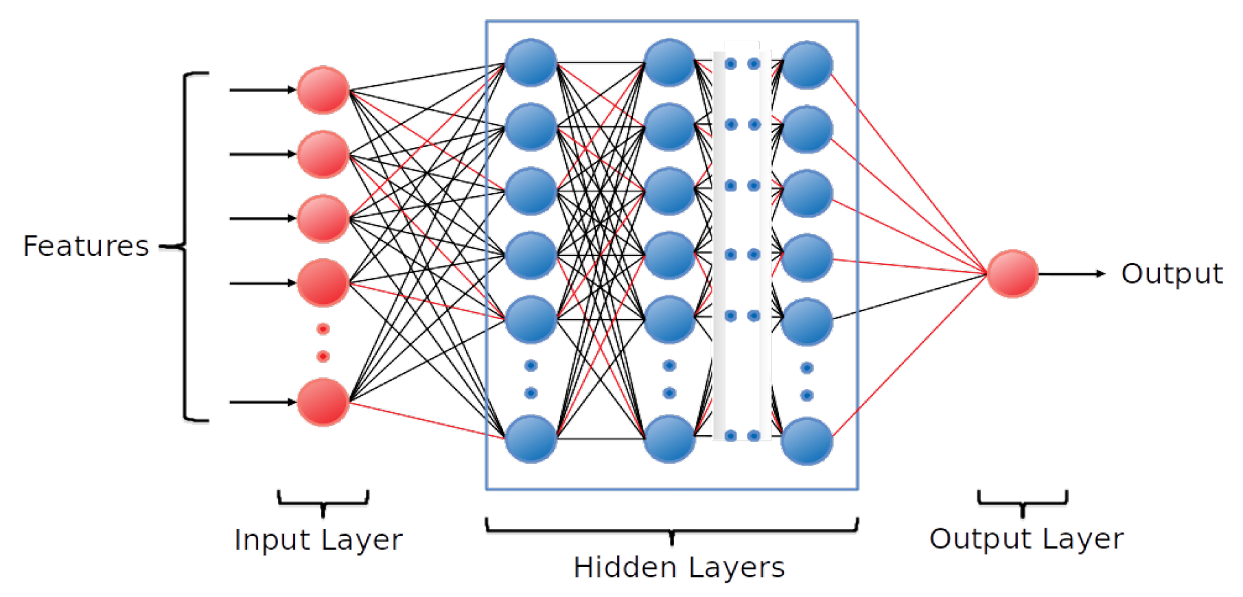
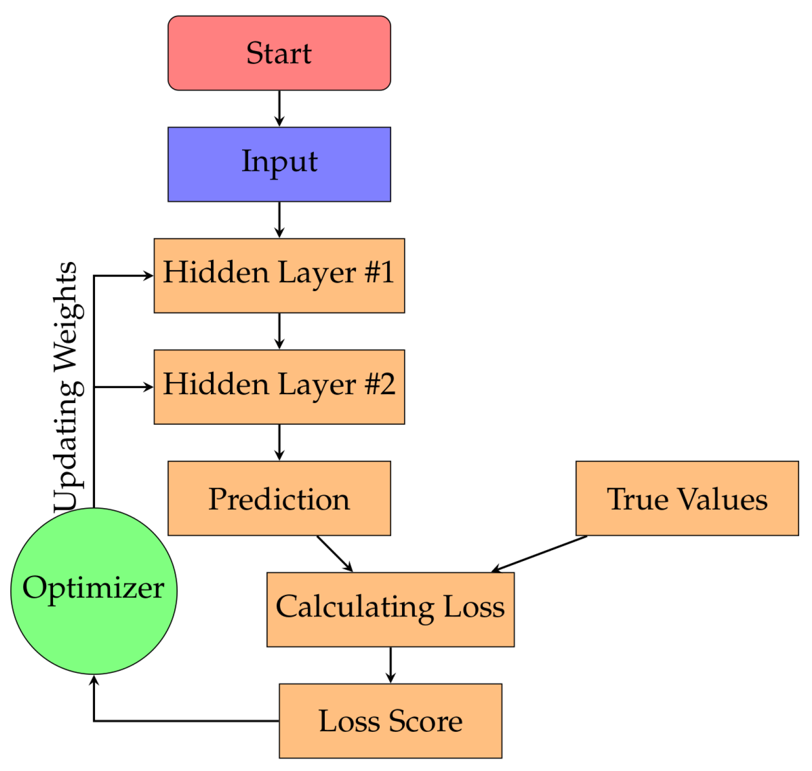
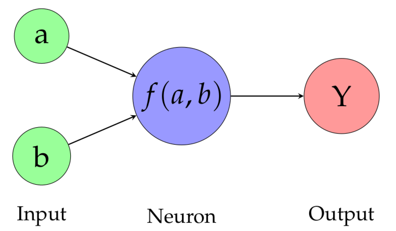
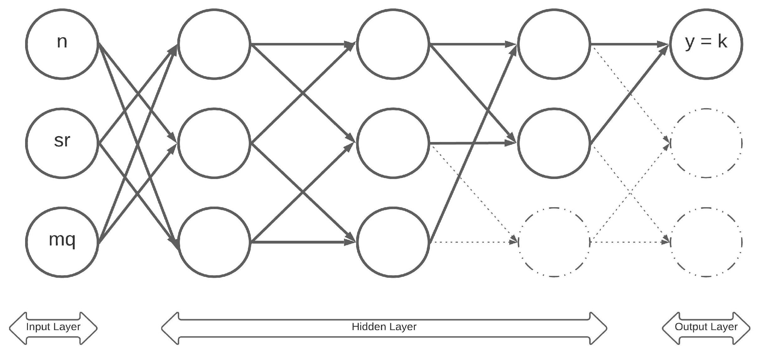
2.1. Artificial Neural Networks (ANN)

The working of an ANN is like that of a human brain. The human brain is composed of billions of nerve cells called neurons. They are connected to another thousand cells by axons. The ANNs are composed of multiple nodes connected by links. It can be said to be a set of algorithms created to prepare the network with numerous layers proficiently. Feed-forward multi-layer perceptron (MLP) is constructed to make the neural network work. Usually, an MLP is a numerical mapping that yields an output from a set of inputs [35,51]. The study utilizes the regression analysis model to predict the output. It includes multiple input variables and a continuous target variable fed into the network. It forms a relationship among these variables to make the model predict an outcome analytically [52]. The schematics of various components of ANN are shown in Figure 2.

Network Construction and Implementation of ANN

The neural network training starts with all the neurons being connected by a random weight and an initializer. This random weight assignment makes the early predictions distant from the actual values. The network weights are updated using an optimizer, and it is passed through the neural network again. This repetitive process of updating weights is called the training of the neural network. A loss function is considered to analyze the training process. A neural network is said to be finally trained when this loss function helps identify the best configuration of the network with the minimum loss. In Figure 2, red connections between neurons show the activated links, and the black connection offers the connection which was not activated. The mean square error (MSE) estimator between the actual and predicted values were chosen for the loss function. To further minimize the loss function, stochastic gradient decent (SGD) algorithm was used. The other loss function optimizer is batch gradient descent (BGD), which can reduce computation time [53]. Based on our previous experiences, we used SGD over BGD, which updates the weights incrementally for each training sample. To optimize the network, we used the back-propagation method. The most commonly used activation functions are the sigmoid, relu and softmax functions. However, the tanh function was our preferred function based on our previous results, as it gives better training performances [54]. Equation (1) shows the zero-centred tanh function ranging from −1 to 1.

$$f\left(x\right)=\frac{e^x-e^{-x}}{e^x+e^{-x}}$$

(1)

The final layer, which has only one neuron, is called the output layer. It is employed with an identity function to show the values received from the previous layer without changing its weights [23]. We used the optimal number of epochs to train the model and avoid over-or under-fitting. A single epoch is a full complete iteration of the neural network. Under-fitting could be overcome by training the network on more epochs and increasing the number of neurons with the hidden layers in the neural network. Conversely, over-fitting appears when a neural network is trained excessively, making the model learn the data instead of generalising it. It usually happens while trying to minimise the error between training and testing data, resulting in a severe validation error of the model. To overcome over-fitting, cross-validation techniques such as K-Fold and regularization techniques can be used [55,56]. However, we used the early stopping method [57] to find an optimal network due to very limited data set of values. It can be seen from our results that when we trained more than the optimal network, it started to show. This is shown in the results from when we tried training, with more differences in training and testing errors.

The inputs of ANN are porosity (n), saturation (Sr) and quartz content (mq), and the output is the thermal conductivity (k) of the sand. Three different ANNs Network I, Network II and Network III are built as explained in the Section 2.

The data set is divided into calibration and validation data for each sample. The working steps of the ANN model are explained with a flow chart shown in Figure 3.

2.2. Group Method of Data Handling (GMDH)

2.2.1. Introduction

The group method of data handling (GMDH) was first introduced by Ivakhnenko as a proper approach for detecting nonlinear systems [43]. GMDH is a self-organising neural network proposed by link. It can be used to model problems with multiple inputs and a single output. The group method data handling (GMDH)-based neural network is similar to ANN but has its differences; ANN has predetermined connections, layers, and neurons in those layers, whereas in GMDH-based neural network, the structure of the network is chosen by the algorithm itself. The GMDH-based neural network, due to its inherent advantages, finds its application in a broad spectrum of domains. It unburdens the researchers from optimising hyper-parameters for identifying the number of layers in a neural network or the number of neurons in it. Many regression problems have been addressed using GMDH based in various engineering and science application as well [44,45].

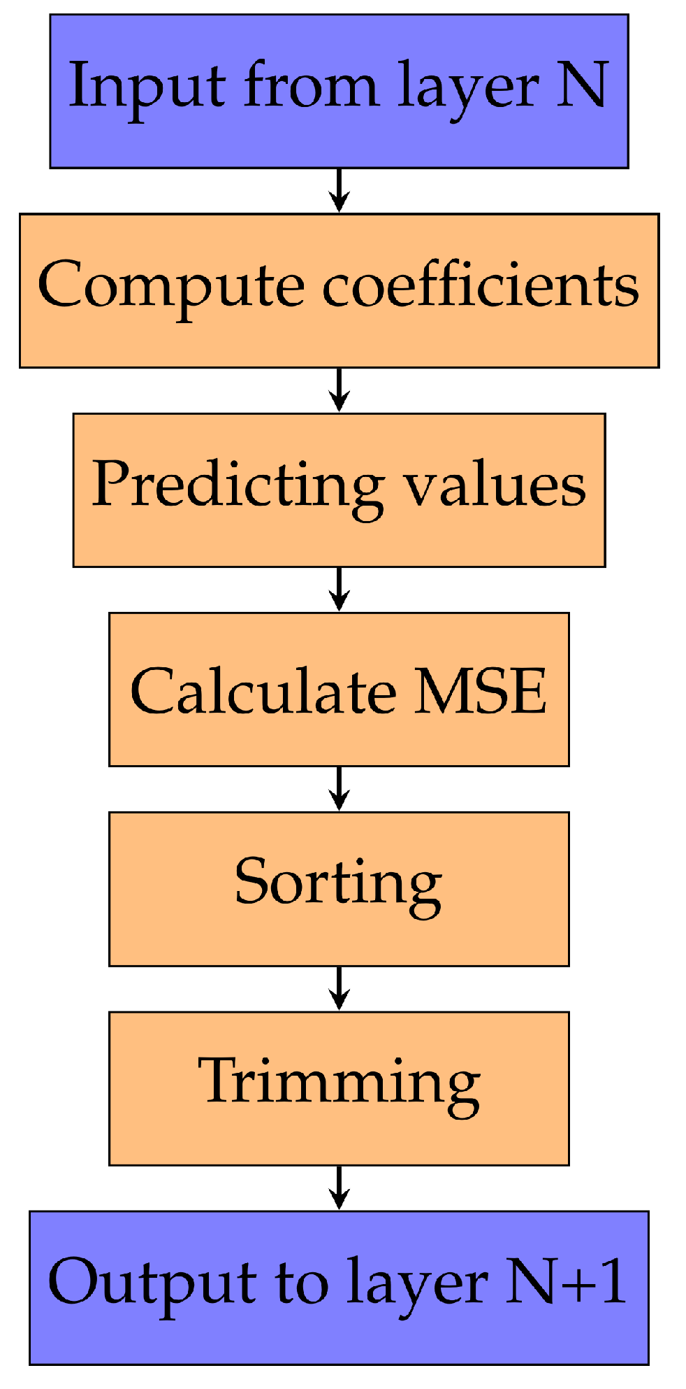
2.2.2. Network Construction and Implementation of GMDH

The GMDH method uses the polynomial transfer functions to relate the input to output with sucessive layers of neurons. In the GMDH network, the neurons depend upon the number of input parameters and the layers are stacked one after the other until the model reaches its maximum accuracy. The connections between the neurons of one layer to neurons of the other layer are chosen to optimise the reliability and accuracy of the network. Each layer is constructed by a neuron which accepts two inputs, applies a polynomial function and spits out an output as shown in the Figure 4 and Equation (2).

$$Y=f(a,b)$$

(2)

The network then uses the minimisation of the difference between the true value $\left(Y\right)$ and the expected value $f(a,b)$ as following

$$\sum _N^{i=1}{\left[f(a,b)-Y)\right]}^2\Rightarrow min$$

(3)

The polynomial relationship between input $(a,b)$ and output Y is taken linearly here considering the size and complexity of the data set (see Equation (4)).

$$f(a,b)=C_0+C_1\ast a+C_2\ast b2+C_3\ast a\ast b.$$

(4)

To calculate the coefficients or weights $(C_0, C_1, C_2$ and $C_3)$ we use Lagrange interpolation as given in the equation below

$$\begin{array}{c}\hfill \left[\begin{array}{cccc}\sum _{i=1}^{m}1& \sum _{i=1}^{m}a& \sum _{i=1}^{m}b& \sum _{i=1}^{m}a·b\\ \sum _{i=1}^{m}a& \sum _{i=1}^m{a}^2& \sum _{i=1}^{m}a·b& \sum _{i=1}^m{a}^2·b\\ \sum _{i=1}^{m}b& \sum _{i=1}^{m}a·b& \sum _{i=1}^m{b}^2& \sum _{i=1}^{m}a·b^2\\ \sum _{i=1}^{m}a·b& \sum _{i=1}^m{a}^2·b& \sum _{i=1}^{m}a·b^2& \sum _{i=1}^m{a}^2·b^2\end{array}\right]\left[\begin{array}{c}{C}_0\\ C_1\\ C_2\\ C_3\end{array}\right]=\left[\begin{array}{c}\sum _{i=1}^{m}Y\\ \sum _{i=1}^{m}a·Y\\ \sum _{i=1}^{m}b·Y\\ \sum _{i=1}^{m}a·b·Y\end{array}\right]\end{array}$$

(5)

The first layer (input layer) has neurons equal to the number of input parameters. In the first hidden layer after the input layer, each neuron in the network accepts the output of two neurons from the previous layer as its inputs. Therefore, the number of neurons in this layer is a function of the number of neurons in the previous layer. This function definition is

$$n\ast (n-1)/2$$

(6)

where n is the number of neurons in the previous layer. This construction of subsequent layers in the network continues in the same fashion.

Each and every neuron in the hidden layer uses a hypothesis defined as a hyper-parameter of the algorithm. After forming a layer, the hypothesis of each neuron is tested. Based on their performance, they are sorted and the output of top-performing neurons is propagated to the next layer. These outputs are used to form the next layer and the same process of forming layers is continued until the addition of layers no longer improves the performance, or until just a single neuron is left.

The three networks, $Network$-I, $Network$-$II$ and $Network$-$III$, are implemented here as well and network was trained and tested.

The available data set was divided into training and test subsets with a ratio of 80/20. During training, the network stopped at the 4th layer as the 5th layer started to over-fit. The graphical representation of the network is shown in Figure 5. The working steps of the GMDH network are shown in Figure 6.

2.3. Gene Expression Programming (GEP)

Gene expression programming (GEP) is an evolutionary algorithm for automatic generation of computer programs and mathematical models. The concept was given by Ferreira [38]. GEP is a special field of evolutionary computation that aims at building programs automatically to solve problems. It uses simple linear chromosomes of fixed length to encode genetic information. Expression trees can be produced from the chromosomes of fixed length through its genotype/phenotype expression system. An example of an expression tree for Equation (7) is displayed in Figure 7.

$$p+q\ast r$$

(7)

Experiments have been conducted to show the cogency of gene expression programming over other conventional methods for prediction. A similar study was conducted to determine the thermal conductivity using gene expression programming in [41]. Many experiments have shown that GEP is more efficient than GP (genetic programming), and that GEP-evolved trees are smaller than GP-evolved trees.

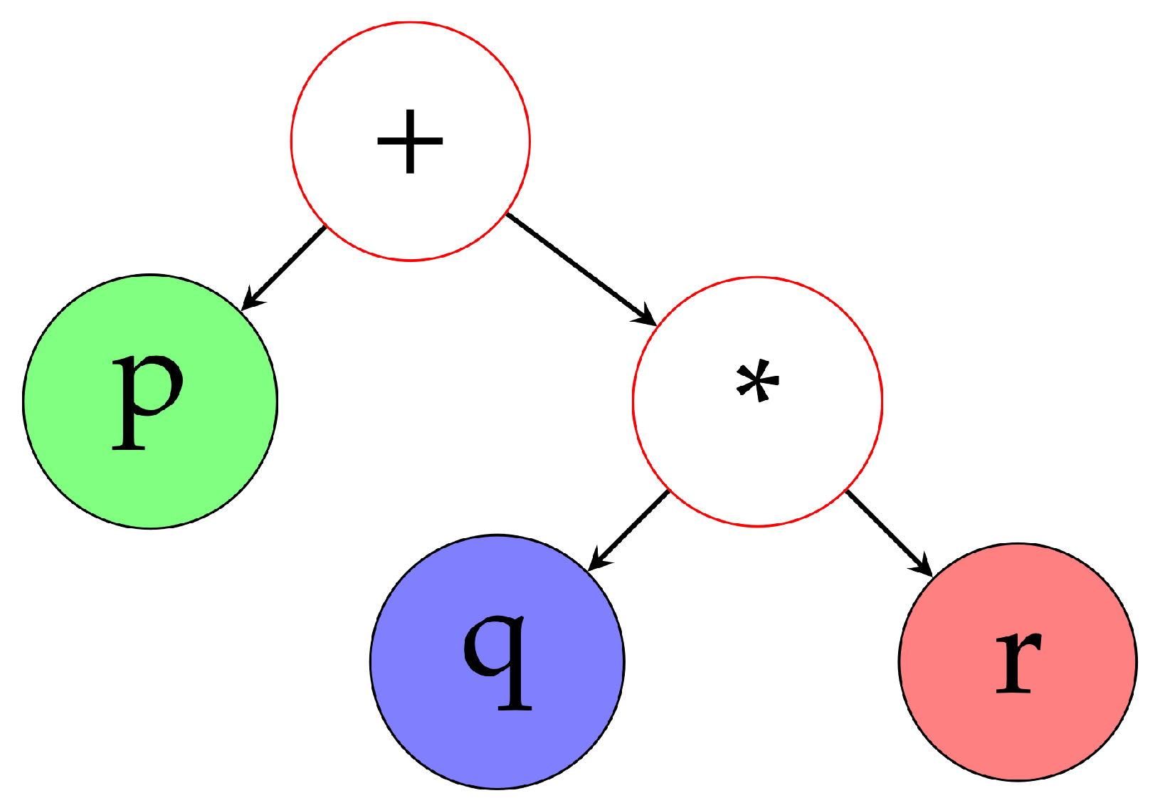
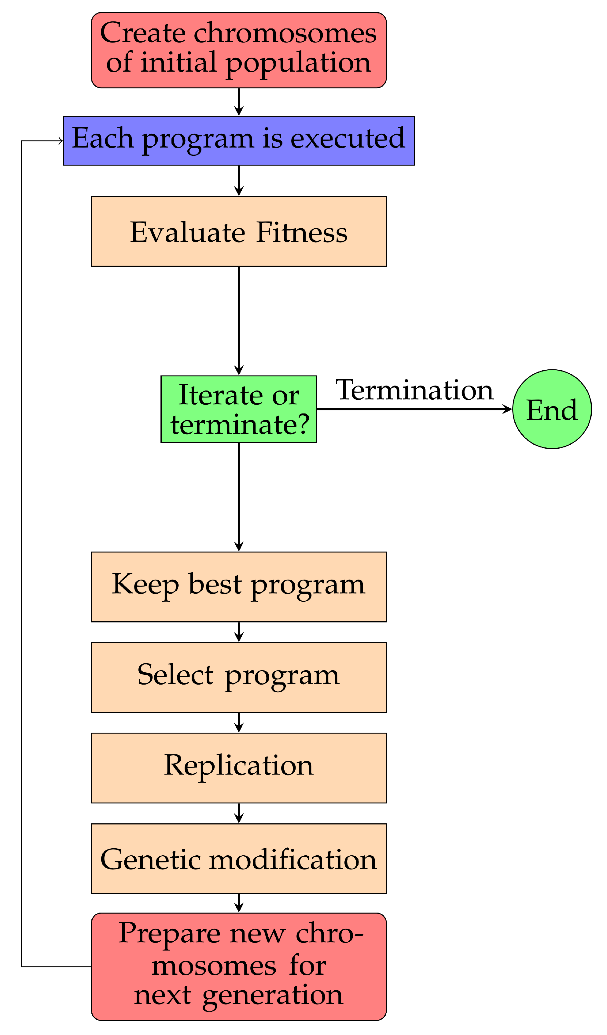
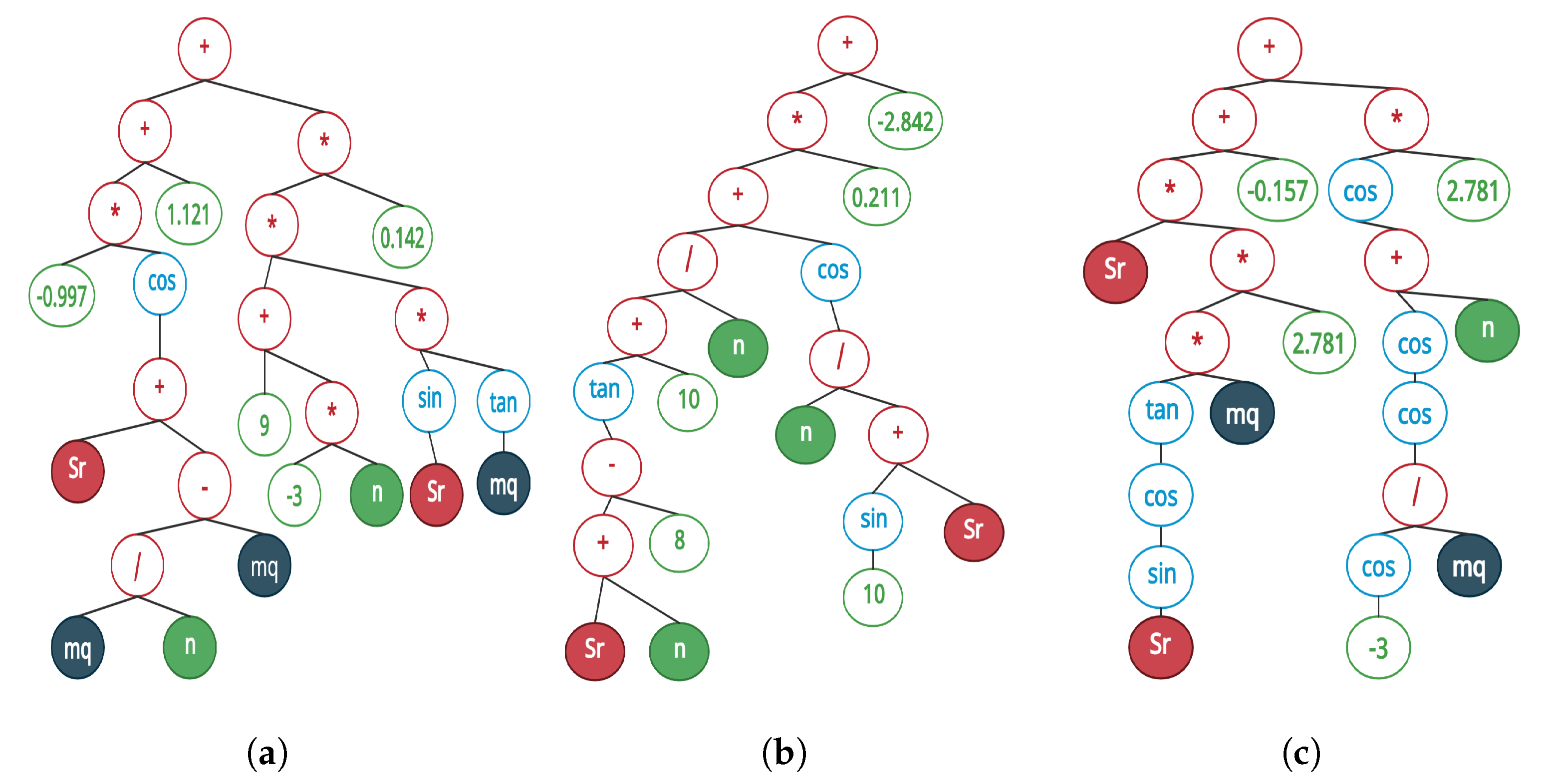
Network Construction and Implementation of GEP

Gene expression programming is a complete genotype/phenotype system that evolves computer programmes contained in fixed-length linear chromosomes. As the expression of each gene always results in valid programmes, the structure of linear chromosomes permits the unrestricted and productive (in the sense that no invalid phenotypes occur) operation of major genetic operators such as mutation, transposition, and recombination.

Symbolic regression is a machine-learning technique or regression analysis that seeks to find an underlying mathematical expression that accurately captures the relationship between variables in a dataset. Genetic programming or gene expression programming are the most common methods for solving symbolic regression (GEP). Constant coefficients are common in mathematical models, which presents a problem for GEP. To address the issue, The GEP-RNC technique uses a common way to handle numerical constants by adding another Dc domain to the genes that are dedicated to the random numerical constant (RNC) evolution.

The flowchart for GEP is shown in Figure 8 [38,40]. The first population’s chromosomes are generated at random. The chromosomes are then expressed and each individual’s fitness is determined using a fitness function. Individuals are then chosen based on their ability to reproduce with alterations, resulting in offspring with new characteristics. Individuals from this new generation go through the same developmental process as their predecessors: genome expression, interaction with the selective environment, and alteration of reproduction. Replication, mutation, transposition and recombination is performed in the reproduction phase. The process is repeated until a solution is found or for a predetermined number of generations.

We used the geppy framework to implement the GEP-RNC algorithm on our dataset. Geppy is an evolutionary algorithm framework specially designed for gene expression programming in python. Geppy is built on top of the excellent evolutionary computation framework DEAP [42] for rapid prototyping and testing of ideas with GEP.

2.4. Error Calculation and Model Selection

Three standard errors are used for computing the accuracy of each neural network for predicting thermal conductivity: the mean square error (MSE), mean absolute error (MAE) and the coefficient of determination ($R^2$). The difference of MSE was chosen as the loss function [53].

$$\mathrm{MSE}=\frac{1}{n}\sum _{i=0}^n{\left(Y_i-\widehat{Y_i}\right)}^2\times 100$$

(8)

$$\mathrm{MAE}=\frac{1}{n}\sum _{t=0}^n|Y_i-\widehat{Y_i}|\times 100$$

(9)

$$R^2=1-\frac{{\sum }_{i=0}^n{\left(Y_i-\widehat{Y_i}\right)}^2}{{\sum }_{i=0}^n{\left(Y_i-\overline{Y}\right)}^2}\times 100$$

(10)

$Y_i$ is the predicted thermal conductivity value, $\overline{Y}$ is the mean value and $\widehat{Y_i}$ is the measured value. n is the number of measurements.

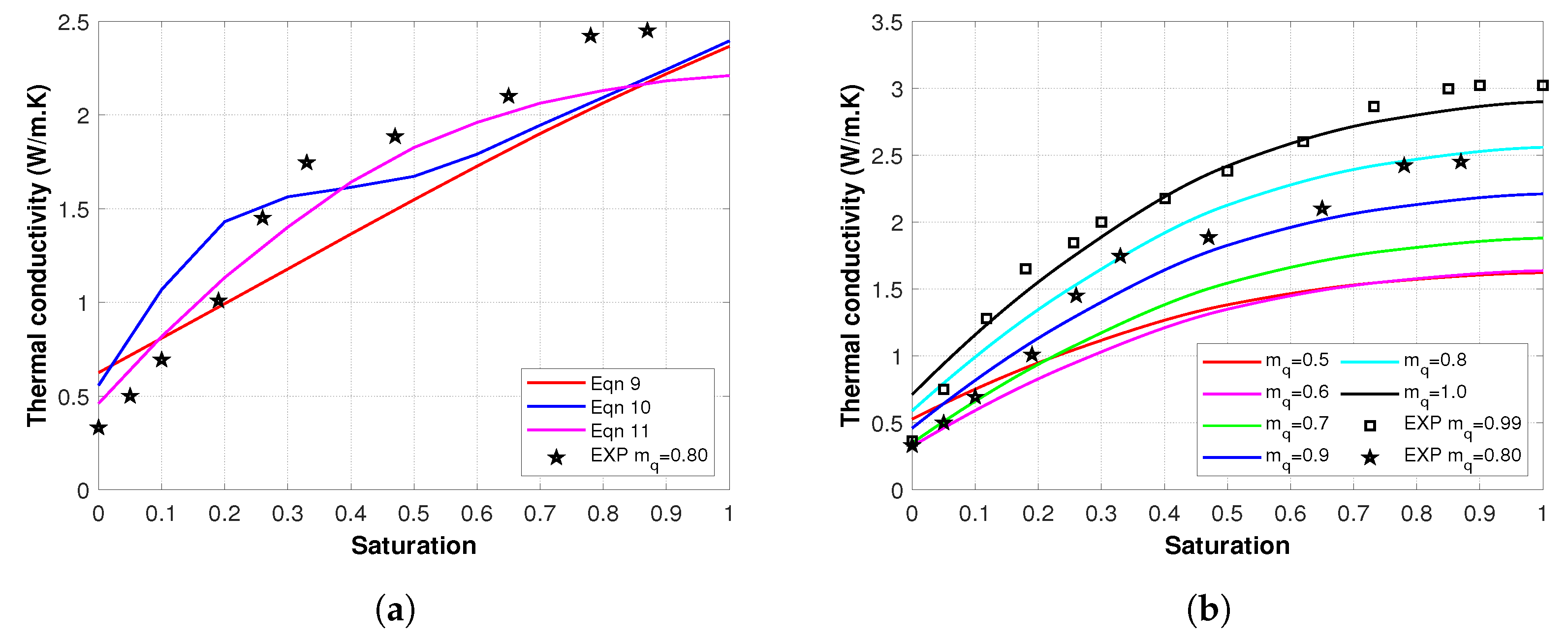
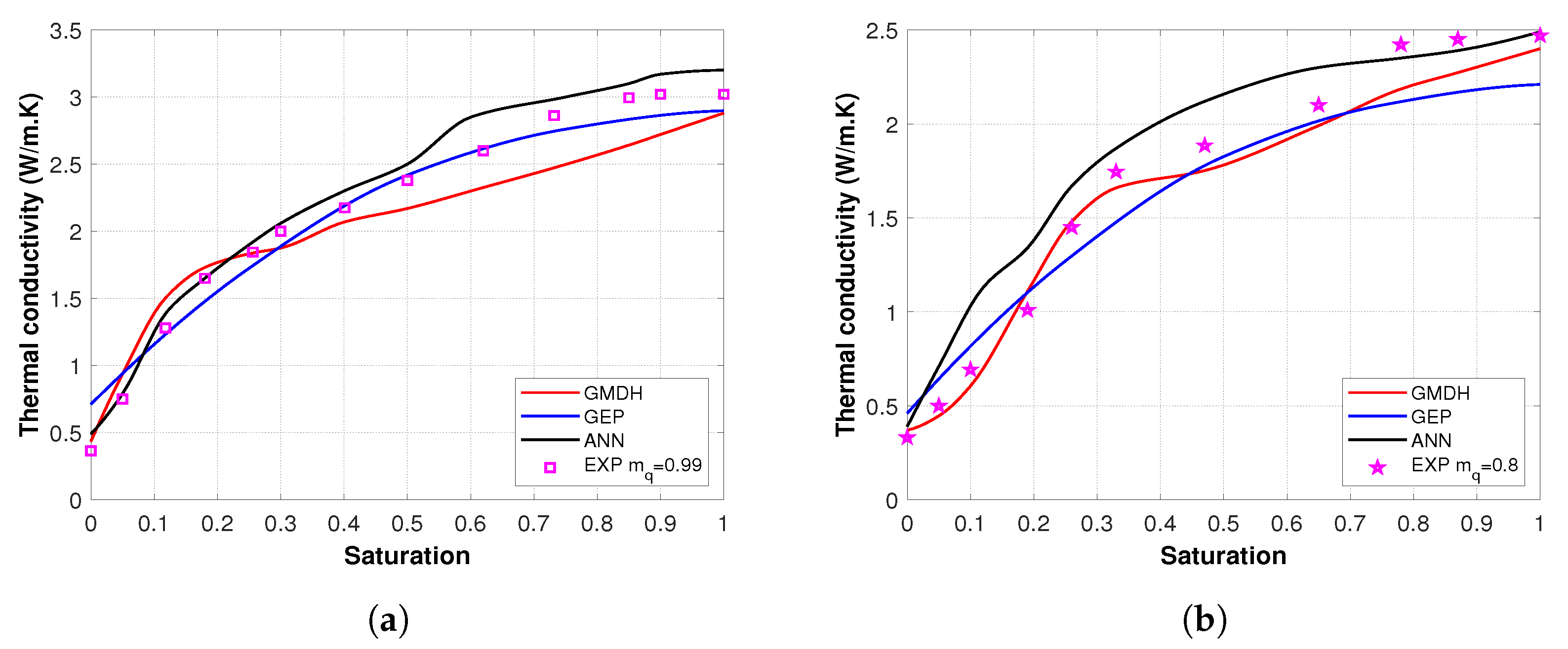
3. Results and Discussion

The three networks, namely, $NetworkI$, $NetworkII$ and $NetworkIII$, as explained in Section 2, are the setup of each type of model. The standard errors were computed, and the best performing model was used to compute the thermal conductivity of two independent samples. The following sections explain the training, testing and validation of each neural network and the intricacies and advantages of each network.

3.1. ANN Results

The three different ANN $Network$I, $Network$$II$ and $Network$$III$ were built considering the two ($n,Sr$) or three ($n,Sr,m_q$) available inputs and one output k. The earlier implementation of ANN is limited in most cases with one single hidden layer and, thus, is limited to accurately predicting for the training data [27,29,30,31,32,33,51]. In addition, no details are provided for the depth of the layers and number of neurons of all the tried combinations. Here, we implemented the ANN based on deep neural network (DNN) feed forward multilayer perceptron (MLP). The neurons in each layer are connected with the corresponding weight factor and activation function. Each neuron is assigned a random initial value. In the subsequent step, weights were updated to minimise the error margin to reach the training output value. Many different combinations of two, three, and four layers of neurons were considered, with neuron numbers ranging between 4 to 16. Similar and dissimilar numbers of neurons werealso considered, resulting in a considerable number of networks. Only the ten best-performing networks are shown here, for brevity. The model training data is classified into two subsets for training and testing with a ratio of 4:1. However, the approach usually runs into a problem known as $overfitting$ [29,32], and, to avoid this, the training data set was further divided into two parts with a ratio of 70:30. The data is subdivided into training, validation, and testing sets, making it easier to cross-validate the model. The implementation involves the use of $Keras$—a deep-learning python library. It provides an easy-to-use, excellent suite of deep-learning functions. Model weight parameters were optimised using the $Adam$ optimiser. This optimiser computes the adaptive learning rate of each parameter. The epoch size for training varied from 400 to 800, and the batch size was fixed to 10.

Table 1. Training, testing and validation results considering $Network$-I. Epochs = 800 and batch size = 10.

S. No.	Layers	Neurons	${\mathit{R}}^2$ %			MSE % (W/m·K)${}^2$			MAE % (W/m·K)			Δ MSE % (W/m·K)${}^2$
			Train	Test	Validation	Train	Test	Validation	Train	Test	Validation	Testing–Training
1	3	8 = 6 = 8	67.118	75.093	65.331	16.520	16.549	15.6	30.086	32.143	31.0	0.029
2	3	6 = 8 = 8	67.285	73.786	66.995	16.436	17.418	14.9	30.190	33.125	30.4	0.982
3	3	8 = 8 = 6	67.735	74.113	67.209	16.210	17.201	14.8	30.188	32.723	30.7	0.991
4	4	8 = 8 = 8 = 8	69.935	74.739	66.704	15.105	16.784	15.0	28.916	31.819	30.1	1.680
5	3	8 = 8 = 8	68.812	73.638	65.356	15.669	17.516	15.6	29.403	33.125	30.9	1.847
6	3	10 = 10 = 10	70.100	74.010	65.235	15.022	17.269	15.7	28.875	33.230	30.4	2.247
7	4	6 = 6 = 6 = 6	70.148	73.563	67.593	14.998	17.566	14.6	28.929	33.262	29.6	2.569
8	3	12 = 12 = 12	70.971	72.473	66.783	14.585	18.291	15.0	28.809	34.069	30.2	3.706
9	4	10 = 10 = 10 = 10	72.888	70.334	64.322	13.621	19.711	16.1	27.216	34.383	30.7	6.090
10	4	12 = 12 = 12 = 12	73.905	68.801	61.769	13.110	20.730	17.2	27.002	36.278	31.3	7.620

shows the $Network$I ANN model with two inputs ($n,Sr$) and variables: number of neurons and hidden layers. From Table 1, it is visible that the network with three hidden layers with 8-6-8 neurons produces the least error.

Table 2. Training, testing and validation results considering $Network$-$II$.

S. No.	Layers	Neurons	${\mathit{R}}^2$ %			MSE % (W/m·K)${}^2$			MAE % (W/m·K)			Δ MSE % (W/m·K)${}^2$
			Train	Test	Validation	Train	Test	Validation	Train	Test	Validation	Testing–Training
1	3	4 = 4 = 4	89.692	91.896	85.526	5.179	5.385	6.5	16.516	16.963	19.6	0.206
2	4	4 = 4 = 4 = 4	89.521	90.886	84.545	5.265	6.056	7.0	16.453	19.214	20.0	0.791
3	3	4 = 6 = 8	90.421	89.204	83.664	4.813	7.174	7.4	15.518	19.133	20.4	2.361
4	3	8 = 8 = 8	91.412	89.644	84.187	4.313	6.880	7.1	14.413	18.713	19.9	2.567
5	3	6 = 6 = 6	91.620	88.532	82.275	4.210	7.620	8.0	14.630	19.444	20.7	3.409
6	3	8 = 8 = 8	92.594	88.792	82.880	3.720	7.447	7.7	13.027	18.307	20.2	3.727
7	3	8 = 6 = 4	92.309	87.197	83.838	3.864	8.507	7.3	13.713	19.750	19.9	4.643
8	4	6 = 6 = 6 = 6	92.710	85.047	84.174	3.662	9.936	7.1	13.514	21.562	18.9	6.273
9	3	10 = 10 = 10	94.562	83.302	80.606	2.732	11.095	8.7	11.398	21.644	20.8	8.363
10	3	12=12=12	95.219	80.201	74.088	2.402	13.156	11.7	10.552	23.912	22.2	10.754

and

Table 3. Training, testing and validation results considering $Network$-$III$.

S. No.	Layers	Neurons	${\mathit{R}}^2$ %			MSE % (W/m·K)${}^2$			MAE % (W/m·K)			Δ MSE % (W/m·K)${}^2$
			Train	Test	Validation	Train	Test	Validation	Train	Test	Validation	Testing–Training
1	3	4 = 4 = 4	89.222	80.189	69.103	6.524	8.380	14.4	19.263	23.078	28.1	1.855
2	3	2 = 2 = 2	87.090	76.474	73.645	7.815	9.951	12.2	21.162	24.863	25.9	2.136
3	3	4 = 4 = 4	90.698	81.269	72.012	5.631	7.923	13.0	17.451	22.585	27.5	2.292
4	3	8 = 8 = 8	92.176	83.306	77.968	4.736	7.061	10.2	15.542	20.768	22.0	2.325
5	3	6 = 6 = 6	92.270	83.216	72.986	4.679	7.099	12.5	15.543	20.959	24.9	2.420
6	4	6 = 6 = 6 = 6	92.904	83.681	76.047	4.295	6.903	11.1	14.769	19.915	23.3	2.607
7	3	8 = 8 = 8	93.542	84.249	71.868	3.909	6.662	13.1	13.886	19.583	24.5	2.753
8	3	8 = 6 = 6	93.097	83.004	68.001	4.179	7.189	14.9	14.633	20.194	26.0	3.010
9	3	10 = 10 = 10	93.533	83.110	70.193	3.915	7.144	13.8	13.980	20.366	24.3	3.230
10	3	12 = 12 = 12	94.867	76.508	73.505	3.107	9.937	12.3	12.430	24.307	22.2	6.830

show the data from $Network$-$II$ and $Network$-$III$ with three input parameters ($n,Sr,m_q$). At first, all the data considered for training the optimal network found had a 4-4-4 configuration. In the second attempt, the data with more than 50% $m_q$ was considered to reduce the data size. Again, the same 4-4-4 network produced the best results. Although the network depth and the number of neurons remain the same in both cases, the training epochs were reduced to half to 400, and the mean difference error margin increased significantly to above $2\%$ (Table 3).

3.2. GMDH Results

The reported work of the GMDH application to compute the ETC is limited to Rizvi et al. [46], where 80 measurements of four different sandy soils were used for training and testing. Soil porosity, saturation and particle size were considered as inputs. The result shows good accuracy for quartz sand but fails to provide reasonable results for other mineralogical compositions. The present work incorporates quartz content as model input, thus improving the model prediction.

GMDH algorithms are characterised by their self-organising property, in which sorting is performed on neurons of a layer. The complexity increases layer after layer gradually until we reach a stopping condition and have the best solution to our objective function. The polynomial mapping functions (quadratic functions) are used in each neuron and fitted by the least-squares method.

The data set was divided into a ratio of 80:20. The standard errors were computed to check the accuracy of the network. The $Network$-I with two inputs showed lower confidence in results. The best performing $Network$$II$ with all training data performed the best with an $R^2$ value of $83.2$ and MSE of $0.086$. The results of all the three networks are given in the

Table 4. The errors resulting from different GMDH models.

Serial No.	${\mathit{R}}^2$ %	MSE % (W/m·K)${}^2$	MAE % (W/m·K)
$Network$-I	78.9	27.60	24.02
$Network$-$II$	83.2	22.60	20.60
$Network$-$III$	81.6	29.19	22.90

.

3.3. GEP Results

The GEP model to compute the ETC is limited to only one previous study where saturation, porosity, quartz content and temperature are considered [41]. The model was trained, and an equation was proposed, but it cannot provide good results at lower saturation (Equation (11)). The model predicts zero thermal conductivity at zero saturation, which is not correct. The model proposed here provides reasonable results for the full range of saturation.

$$k={\left(2S_r\right)}^{n(0.6-S_r)}·{\sqrt{S_r}}^{n(n-S_r+2.79)}·\left(\frac{1}{4}{(\frac{6.58+T}{2})}^{\frac{1}{3}}+\frac{m_q}{16}+0.49\right)$$

(11)

The dataset was divided into an 80:20 ratio for training and test set. The three expression trees were constructed from $Network$-I, $Network$-$II$ and $Network$-$III$.

Firstly, different GEP RNC model configuration parameters were decided, including the primitive set. The values of different parameters are displayed in

Table 5. GEP model configuration and parameters.

Parameter	Values
Function set	+, −, *, /, sin, cos, tan
Head length	7
Number of genes	2
RNC array length	10
Mutation rate	0.065
Inverse rate	0.1
One-point recombination rate	0.3
Two-point recombination rate	0.3
Population size	200
Number of generations	110

.

The GEP-RNC algorithm was implemented on the three networks using the configuration given in Table 5, and the following equations and expression trees were obtained.

The GEP expression for $Network$-I is shown in Figure 9a, and the corresponding equation is given by Equation (9).

$$k=\frac{0.211}{n}(ncos(\frac{n}{Sr+sin\left(10\right)})+tan(n+Sr-8)+10)-2.842$$

(12)

The GEP expression for $Network$-$II$ is shown in Figure 9b, and the corresponding equation is given by Equation (10).

$$k=0.142(9-3n)sin\left(Sr\right)tan{m}_q-0.997cos(-m_q+\frac{m_q}{n}+Sr)+1.121$$

(13)

The GEP expression for $Network-III$ is shown in Figure 9c and the corresponding equation is given by Equation (11).

$$k=2.781m_{q}Srtan(cos(sin\left(Sr\right)))+2.781cos(n+cos(cos(\frac{cos\left(3\right)}{m_q})))-0.157$$

(14)

The standard error were calculated and are reported in the

Table 6. GEP model error calculation of each network.

Objective	${\mathit{R}}^2$ %		MSE % (W/m·K)${}^2$		MAE % (W/m·K)
	Train	Test	Train	Test	Train	Test
I	84.6759	76.7418	8.0559	11.1374	20.4339	24.0244
II	69.5608	55.0665	16.0020	21.5169	31.3082	33.8458
III	80.5164	79.1439	10.4814	12.7152	23.8305	29.7945

.

To test the developed equations, the measurement performed with sand with 80% quartz content ($m_q$) was used. The result is plotted in Figure 10a. The Equation (9) corresponding to $Network$-I with two inputs shows a linear trend. The equation fails to predict the behaviour at lower and higher saturations and the nonlinear dependency of saturation on the thermal conductivity value.

$Network$-$II$ showed a significant improvement when adding one more input parameter and can show nonlinear behaviour at a lower saturation range but flipped to linear behaviour at higher saturations (see Figure 10a and Equation (10)).

Equation (11) corresponding to $Network$-$III$ showed typical nonlinear behaviour and a good correlation at lower and middle saturation regions (see Equation (10), Figure 10a) but failed at higher saturations. However, the performance of $Network$-$III$ is better than $Network$-$II$ despite being only trained with $m_q$ values greater than 0.5. Therefore, Equation (10) corresponding to $Network$-$II$ was considered for further computation.

To test the performance of Equation (10), one additional experimental value was added to the study with an $m_q$ value of 99%. The quartz content of Equation (10) was varied between 0.5 to 1.0 with an interval of 0.1, and the lines were plotted. The equation showed good correlation for both 80% and 99% quartz content.

3.4. Comparison among Methods

The best performing network of each method was chosen and used to predict the thermal conductivity of two different sands with $m_q$ values of 0.9 and 0.8. The ANN showed good agreement for sand with a $m_q$ value of 0.9; however, the accuracy dropped marginally for $m_q$ of 0.8 (Figure 11b). The GEP equation from $Netwrok$$III$ showed a good agreement at mid-range saturations for $m_q$ 0.9; however, the error at lower and higher saturations was significant. For $m_q$ of 0.8, the prognosis depreciates at both the mid and higher saturation ranges. The GMDH model performed well at lower saturation ranges but under-predicted the thermal conductivity value at higher saturations for $m_q$ of 0.9. A similar trend was observed for $m_q$ of 0.8, shown in Figure 11b, where the GMDH underperformed at higher saturation ranges.

The above results show that the ANN network outperformed the GEP and GMDH networks. However, due to the GEP equation’s simplicity, it has more direct application for practical engineering applications. The GMDH model has the advantage of quick model training with a small data set and parameter sensitivity ranking.

4. Conclusions

In this paper, we presented three neural network approaches to estimate the thermal conductivity of the soil. The network models were chosen based on accuracy, training speed and data requirement, input parameter sensitivity marker and ability to present a simple mathematical formula. The artificial neural network with $Network$-$II$ showed a superior prediction ability with three inputs and MSE value of $20.6\%$ and a $R^2$ value of $89.6\%$ and $91.9\%$ for training and testing, respectively. The group method of data handling showed the best result with $Network$-$II$ as well; however, the $R^2$ value depreciated to $83.2\%$ and MSE to $22.6\%$. The gene expression programming provided the best fitting equation with $Network$-$III$ with an MSE value of $12.0\%$ and $R^2$ value of $80.5\%$ and $79.1\%$ for training and testing, respectively. The networks could be improved by providing more dispersed data to avoid bias. Further studies will incorporate the effect of temperature on soil thermal conductivity and shall be reported elsewhere. The method presented here is generic and could be applied with minor changes to any other field of study.

References

1. Chen, S.X. Thermal conductivity of sands. Heat Mass Transf. 2008, 44, 1241–1246. [Google Scholar] [CrossRef]
2. Lu, J.; Wan, X.; Yan, Z.; Qiu, E.; Pirhadi, N.; Liu, J. Modeling thermal conductivity of soils during a freezing process. Heat Mass Transf. 2022, 58, 283–293. [Google Scholar] [CrossRef]
3. Liang, B.; Chen, M.; Guan, J. Experimental assessment on the thermal and moisture migration of sand-based materials combined with kaolin and graphite. Heat Mass Transf. 2021, 58, 1075–1089. [Google Scholar] [CrossRef]
4. Zhu, F.; Zhou, Y.; Zhu, S. Experimental study on heat transfer in soil during heat storage and release processes. Heat Mass Transf. 2021, 57, 1485–1497. [Google Scholar] [CrossRef]
5. Yildiz, A.; Stirling, R.A. Ground heat exchange potential of Green Infrastructure. Geothermics 2022, 101, 102351. [Google Scholar] [CrossRef]
6. Ahmad, S.; Rizvi, Z.H.; Arp, J.C.C.; Wuttke, F.; Tirth, V.; Islam, S. Evolution of Temperature Field around Underground Power Cable for Static and Cyclic Heating. Energies 2021, 14, 8191. [Google Scholar] [CrossRef]
7. Liu, L.; He, H.; Dyck, M.; Lv, J. Modeling thermal conductivity of clays: A review and evaluation of 28 predictive models. Eng. Geol. 2021, 288, 106107. [Google Scholar] [CrossRef]
8. Sun, Q.; Lyu, C.; Zhang, W. The relationship between thermal conductivity and electrical resistivity of silty clay soil in the temperature range -20 C to 10 C. Heat Mass Transf. 2020, 56, 2007–2013. [Google Scholar] [CrossRef]
9. Bai, B.; Wang, Y.; Rao, D.; Bai, F. The Effective Thermal Conductivity of Unsaturated Porous Media Deduced by Pore-Scale SPH Simulation. Front. Earth Sci. 2022, 10, 943853. [Google Scholar] [CrossRef]
10. He, H.; Dyck, M.F.; Horton, R.; Ren, T.; Bristow, K.L.; Lv, J.; Si, B. Development and application of theheat pulse method for soil physicalmeasurements. Rev. Geophys. 2018, 56, 567–620. [Google Scholar] [CrossRef]
11. Ge, R.; Zheng, Y. Measuring effective thermal conductivity of micro-particle porous materials in fixed bed by thermal probe method. Heat Mass Transf. 2020, 56, 2681–2691. [Google Scholar] [CrossRef]
12. Hailemariam, H.; Shrestha, D.; Wuttke, F.; Wagner, N. Thermal, dielectric, behaviour of fine-grained soils. Environ. Geotech. 2017, 4, 79–93. [Google Scholar] [CrossRef]
13. Zhang, W.; Bai, R.; Xu, X.; Liu, W. An evaluation of soil thermal conductivity models based on the porosity and degree of saturation and a proposal of a new improved model. Int. Commun. Heat Mass Transf. 2021, 129, 105738. [Google Scholar] [CrossRef]
14. Gori, F.; Corasaniti, S. New model to evaluate the effective thermal conductivity of three-phase soils. Int. Commun. Heat Mass Transf. 2013, 47, 1–6. [Google Scholar] [CrossRef]
15. Haigh, S.K. Thermal conductivity of sands. Géotechnique 2012, 62, 617–625. [Google Scholar] [CrossRef]
16. He, H.; Liu, L.; Dyck, M.; Si, B.; Lv, J. Modelling dry soil thermal conductivity. Soil Tillage Res. 2021, 213, 105093. [Google Scholar] [CrossRef]
17. Tarnawski, V.R.; Tsuchiya, F.; Coppa, P.; Bovesecchi, G. Volcanic soils: Inverse modeling of thermal conductivity data. Int. J. Thermophys. 2019, 40, 14–38. [Google Scholar] [CrossRef]
18. El Moumen, A.; Kanit, T.; Imad, A.; El Minor, H. Computational thermal conductivity in porous materials using homogenization techniques: Numerical and statistical approaches. Comput. Mater. Sci. 2015, 97, 148–158. [Google Scholar] [CrossRef]
19. He, J.; Liu, Q.; Wu, Z.; Xu, X. Modelling transient heat conduction of granular materials by numerical manifold method. Eng. Anal. Bound. Elem. 2018, 86, 45–55. [Google Scholar] [CrossRef]
20. Shrestha, D.; Rizvi, Z.H.; Wuttke, F. Effective thermal conductivity of unsaturated granular geocomposite using lattice element method. Heat Mass Transf. 2019, 55, 1671–1683. [Google Scholar] [CrossRef]
21. Lydzba, D.; Rozanski, A.; Rajczakowska, M.; Stefaniuk, D. Random checkerboard based homogenization for estimating effective thermal conductivity of fully saturated soils. J. Rock Mech. Geotech. Eng. 2017, 9, 18–28. [Google Scholar] [CrossRef]
22. Kiani-Oshtorjani, M.; Jalali, P. Thermal discrete element method for transient heat conduction in granular packing under compressive forces. Int. J. Heat Mass Transf. 2019, 145, 118753. [Google Scholar] [CrossRef]
23. Rizvi, Z.H.; Zaidi, H.H.; Akhtar, S.J.; Sattari, A.S.; Wuttke, F. Soft and hard computation methods for estimation of the effective thermal conductivity of sands. Heat Mass Transf. 2020, 56, 1947–1959. [Google Scholar] [CrossRef]
24. Yun, T.S.; Evans, T.M. Three-dimensional random network model for thermal conductivity in particulate materials. Comput. Geotech. 2010, 37, 991–998. [Google Scholar] [CrossRef]
25. Sattari, A.S.; Rizvi, Z.H.; Motra, H.B.; Wuttke, F. Meso-scale modeling of heat transport in a heterogeneous cemented geomaterial by lattice element method. Granul. Matter. 2017, 19, 66. [Google Scholar] [CrossRef]
26. Govender, N. A DEM study on the thermal conduction of granular material in a rotating drum using polyhedral particles on GPUs. Chem. Eng. Sci. 2022, 252, 117491. [Google Scholar] [CrossRef]
27. Li, K.-Q.; Liu, Y.; Kang, Q. Estimating the thermal conductivity of soils using six machine learning algorithms. Int. Commun. Heat Mass Transf. 2022, 136, 106139. [Google Scholar] [CrossRef]
28. Zhao, T.; Liu, S.; Xu, J.; He, H.; Wang, D.; Horton, R.; Liu, G. Comparative analysis of seven machine learning algorithms and five empirical models to estimate soil thermal conductivity. Agric. For. Meteorol. 2022, 323, 109080. [Google Scholar]
29. Kardani, N.; Bardhan, A.; Samui, P.; Nazem, M.; Zhou, A.; Armaghani, D.J. A novel technique based on the improved firefly algorithm coupled with extreme learning machine (ELM-IFF) for predicting the thermal conductivity of soil. Eng. Comput. 2021, 38, 3321–3340. [Google Scholar] [CrossRef]
30. Zhu, C.Y.; He, Z.Y.; Du, M.; Gong, L.; Wang, X. Predicting the effective thermal conductivity of unfrozen soils with various water contents based on artificial neural network. Nanotechnology 2022, 33, 065408. [Google Scholar] [CrossRef]
31. Singh, R.; Bhoopal, R.; Kumar, S. Prediction of effective thermal conductivity of moist porous materials using artificial neural network approach. Build. Environ. 2011, 46, 2603–2608. [Google Scholar] [CrossRef]
32. Zhang, N.; Zou, H.; Zhang, L.; Puppala, A.J.; Liu, S.; Cai, G. A unified soil thermal conductivity model based on artificial neural network. Int. J. Therm. Sci. 2020, 155, 106414. [Google Scholar] [CrossRef]
33. Zhang, T.; Wang, C.-J.; Liu, S.-Y.; Zhang, N.; Zhang, T.-W. Assessment of soil thermal conduction using artificial neural network models. Cold Reg. Sci. Technol. 2020, 169, 102907. [Google Scholar] [CrossRef]
34. Wei, H.; Zhao, S.; Rong, Q.; Bao, H. Predicting the effective thermal conductivities of composite materials and porous media by machine learning methods. Int. J. Heat Mass Transf. 2018, 127, 908–916. [Google Scholar] [CrossRef]
35. Goodfellow, I.; Bengio, Y.; Courville, A. Deep Learning; MIT Press: Cambridge, MA, USA, 2016; pp. 95–96. [Google Scholar]
36. Wang, C.; Cai, G.; Liu, X.; Wu, M. Prediction of soil thermal conductivity based on Intelligent computing model. Heat Mass Transf. 2022, 58, 1695–1708. [Google Scholar] [CrossRef]
37. Go, G.H.; Lee, S.R.; Kim, Y.S. A reliable model to predict the thermal conductivity of unsaturated weathered granite soils. Int. Commun. Heat Mass Transf. 2016, 74, 82–90. [Google Scholar] [CrossRef]
38. Ferreira, C. Gene expression programming: A new adaptive algorithm for solving problems. Complex Syst. 2001, 13, 87–129. [Google Scholar]
39. Ferreira, C. Gene expression programming: Mathematical modeling by an artificial intelligence. Stud. Comput. Intell. 2006, 21, 29–54. [Google Scholar]
40. Zhong, J.; Feng, L.; Ong, Y.-S. Gene expression programming: A survey. IEEE Comput. Intell. Mag. 2017, 12, 54–72. [Google Scholar] [CrossRef]
41. Zhang, R.; Xue, X. A new model for prediction of soil thermal conductivity. Int. Commun. Heat Mass Transf. 2021, 129, 105661. [Google Scholar] [CrossRef]
42. Felix-Antoine, F.; De Rainville, F.M.; Gardner, M.A.; Gagne, C.; Parizeau, M. DEAP: Evolutionary Algorithms Made Easy. J. Mach. Learn. Res. 2012, 13, 2171–2175. [Google Scholar]
43. Ivakhnenko, A.G.; Savchenko, E.A. Problems of future GMDH algorithms development. Syst. Anal. Model. Simul. 2003, 43, 1301–1309. [Google Scholar] [CrossRef]
44. Ansari, M.F.; Hussain, A.; Ansari, M.A. Experimental studies and model development of flow over Arched Labyrinth Weirs using GMDH method. J. Appl. Water Eng. Res. 2021, 9, 265–276. [Google Scholar] [CrossRef]
45. Mrugalski, M. An unscented Kalman filter in designing dynamic GMDH neural networks for robust fault detection. Int. J. Appl. Math. Comput. Sci. 2013, 23, 157–169. [Google Scholar] [CrossRef]
46. Rizvi, Z.H.; Husain, S.M.B.; Haider, H.; Wuttke, F. Effective thermal conductivity of sands estimated by Group Method of Data Handling (GMDH). Mater. Today Proc. 2020, 26, 2103–2107. [Google Scholar] [CrossRef]
47. Tarnawski, V.R.; Momose, T.; McCombie, M.L.; Leong, W.H. Canadian field soils III. Thermal-conductivity data and modeling. Int. J. Thermophys. 2015, 36, 119–156. [Google Scholar] [CrossRef]
48. Zhang, N.; Yu, X.B.; Pradhan, A.; Puppala, A.J. Thermal conductivity of quartz sands by thermo-time domain reflectometry probe and model prediction. J. Mater. Civ. Eng. 2015, 27, 04015059–04015068. [Google Scholar] [CrossRef]
49. Hailemariam, H.; Shrestha, D.; Wuttke, F. Steady state vs transient thermal conductivity of soils. In Energy Geotechnics; Taylor Francis Group: Abingdon, UK, 2016. [Google Scholar]
50. Tarnawski, V.R.; Momose, T.; Leong, W.H. Assessing the impact of quartz content on the prediction of soil thermal conductivity. Geotechnique 2009, 59, 331. [Google Scholar] [CrossRef]
51. Li, K.Q.; Kang, Q.; Nie, J.Y.; Huang, X.W. Artificial neural network for predicting the thermal conductivity of soils based on a systematic database. Geothermics 2022, 103, 102416. [Google Scholar] [CrossRef]
52. Raschka, S.; Mirjalili, V. Python Machine Learning; Packt Publishing Ltd.: Birmingham, UK, 2018; Volume 44, pp. 3–5. [Google Scholar]
53. Rizvi, Z.H.; Akhtar, S.J.; Sabeeh, W.T.; Wuttke, F. Effective thermal conductivity of unsaturated soils based on deep learning algorithm. In Proceedings of the E3S Web of Conferences, La Jolla, CA, USA, 20–23 September 2020; Volume 205, p. 04006. [Google Scholar]
54. Nwankpa, C.E.; Ijomah, W.; Gachagan, A.; Marshall, S. Activation functions: Comparison of trends in practice and research for deep learning. In Proceedings of the 2nd International Conference on Computational Sciences and Technologies (INCCST 20), MUET, Jamshoro, Pakistan, 17–19 December 2020. [Google Scholar]
55. Ghojogh, B.; Crowley, M. The theory behind overfitting, cross validation, regularization, bagging, and boosting: Tutorial. arXiv 2019, arXiv:1905.12787. [Google Scholar]
56. Cogswell, M.; Ahmed, F.; Girshick, R.; Zitnick, L.; Batra, D. Reducing overfitting in deep networks by decorrelating representations. arXiv 2015, arXiv:1511.06068. [Google Scholar]
57. Ying, X. An overview of overfitting and its solutions. J. Phys. Conf. Ser. 2019, 1168, 022022. [Google Scholar] [CrossRef]
Figure 1. The thermal conductivity database with varying degrees of saturation and porosity used for training, testing and validation of models. The variation in quartz content of the sample is shown with the legend colour bar ranging from 0.1 to 1.
Mathematics 10 03957 g001
Figure 2. An artificial neural network with multiple hidden layers.
Mathematics 10 03957 g002
Figure 3. The flowchart of the learning cycle for training the ANN.
Mathematics 10 03957 g003
Figure 4. Basic structure of neuron in GMDH-based neural network.
Mathematics 10 03957 g004
Figure 5. GMDH Model with three inputs and one output.
Mathematics 10 03957 g005
Figure 6. The training steps of the GMDH network.
Mathematics 10 03957 g006
Figure 7. The expression tree of Equation (7).
Mathematics 10 03957 g007
Figure 8. The model working steps of the GEP network.
Mathematics 10 03957 g008
Figure 9. The GEP Expression tree from three configurations of input data: (a) expression tree for N e t w o r k -I, (b) expression tree for N e t w o r k - I I , and (c) expression tree for N e t w o r k - I I I .
Mathematics 10 03957 g009
Figure 10. Thermal conductivity predection based on GEP. (a) Thermal conductivity estimation from Equations (12)–(14) plotted against experiment result for m q of 0.8 (b) with values of m q ranging between 0.5–1.0 in Equation (14) and experiment result of m q 0.8 and 0.99 of two different sands.
Mathematics 10 03957 g010
Figure 11. Model prediction of three different networks and experimental results (a) for quartz content m q 0.8 (b) m q 0.99.
Mathematics 10 03957 g011