


PN-BBN: A Petri Net-Based Bayesian Network for Anomalous Behavior Detection

1
School of Mathematics and Big Data, Anhui University of Science and Technology, Huainan 232001, China
2
Anhui Province Engineering Laboratory for Big Data Analysis and Early Warning Technology of Coal Mine Safety, Huainan 232001, China
*
Author to whom correspondence should be addressed.
Mathematics 2022, 10(20), 3790; https://doi.org/10.3390/math10203790
Submission received: 9 September 2022
/
Revised: 8 October 2022
/
Accepted: 11 October 2022
/
Published: 14 October 2022
(This article belongs to the Topic Machine and Deep Learning)
Abstract
:Business process anomalous behavior detection reveals unexpected cases from event logs to ensure the trusted operation of information systems. Anomaly behavior is mainly identified through a log-to-model alignment analysis or numerical outlier detection. However, both approaches ignore the influence of probability distributions or activity relationships in process activities. Based on this concern, this paper incorporates the behavioral relationships characterized by the process model and the joint probability distribution of nodes related to suspected anomalous behaviors. Moreover, a Petri Net-Based Bayesian Network (PN-BBN) is proposed to detect anomalous behaviors based on the probabilistic inference of behavioral contexts. First, the process model is filtered based on the process structure of the process activities to identify the key regions where the suspected anomalous behaviors are located. Then, the behavioral profile of the activity is used to prune it to position the ineluctable paths that trigger these activities. Further, the model is used as the architecture for parameter learning to construct the PN-BBN. Based on this, anomaly scores are inferred based on the joint probabilities of activities related to suspected anomalous behaviors for anomaly detection under the constraints of control flow and probability distributions. Finally, PN-BBN is implemented based on the open-source frameworks PM4PY and PMGPY and evaluated from multiple metrics with synthetic and real process data. The experimental results demonstrate that PN-BBN effectively identifies anomalous process behaviors and improves the reliability of information systems.
Keywords:
anomalous behavior detection; petri net-based bayesian network; probabilistic inference; behavior profile; behavior contextMSC:
68Q87; 62F151. Introduction
Digital information systems use process models and other business specifications to guide the safe and trusted operation of the system while storing operational records in an event log. However, the actual execution process does not always conform to the planning scheme, and thus unexpected behavior occurs. Therefore, anomalous behavior detection techniques are widely used in business process management and play an essential role in ensuring business processes’ correct and orderly execution [1]. There is no strict definition for how to define anomalous behavior formally, but some consensus has been developed: (1) they differ from normal behavior in specific characteristics; and (2) they occur much less frequently than usual behavior [2]. Based on this consensus, a variety of anomalous behaviors can be defined, such as intrusion detection in network environments [3], fraud detection in e-commerce [4], and data leakage prevention [5]. The effective detection of these abnormal behaviors means the system can stop the damage in time and reduce the impact caused by deviant behaviors.
Automated anomalous behavior detection requires the ability to determine whether abnormal behavior is occurring in the system by analyzing the operational patterns of the raw data. Standard anomalous behavior detection methods are currently divided into data-centric and model-centric approaches. The former focuses on identifying non-normal data by analyzing numerical differences, and this idea is widely used in data mining. For example, Liu et al. constructed an effective anomaly detection method based on data-level constraints [6]. Using sparse operations to obtain representations of high-dimensional data, domain information in the form of similarity matrices can be brought, based on which anomalies can be discerned using graph clustering techniques. The latter (the model-centric approach) focuses on analyzing the interactions and constraints between different events in a business process to detect anomalous behavior by locating contradictory points in the business logic. These two approaches are sensitive to numerical and behavioral anomalies, respectively, and each plays a vital role in anomaly detection. However, they lack the description of multiple activity–behavior relationships and the joint probability distribution of activity contexts.
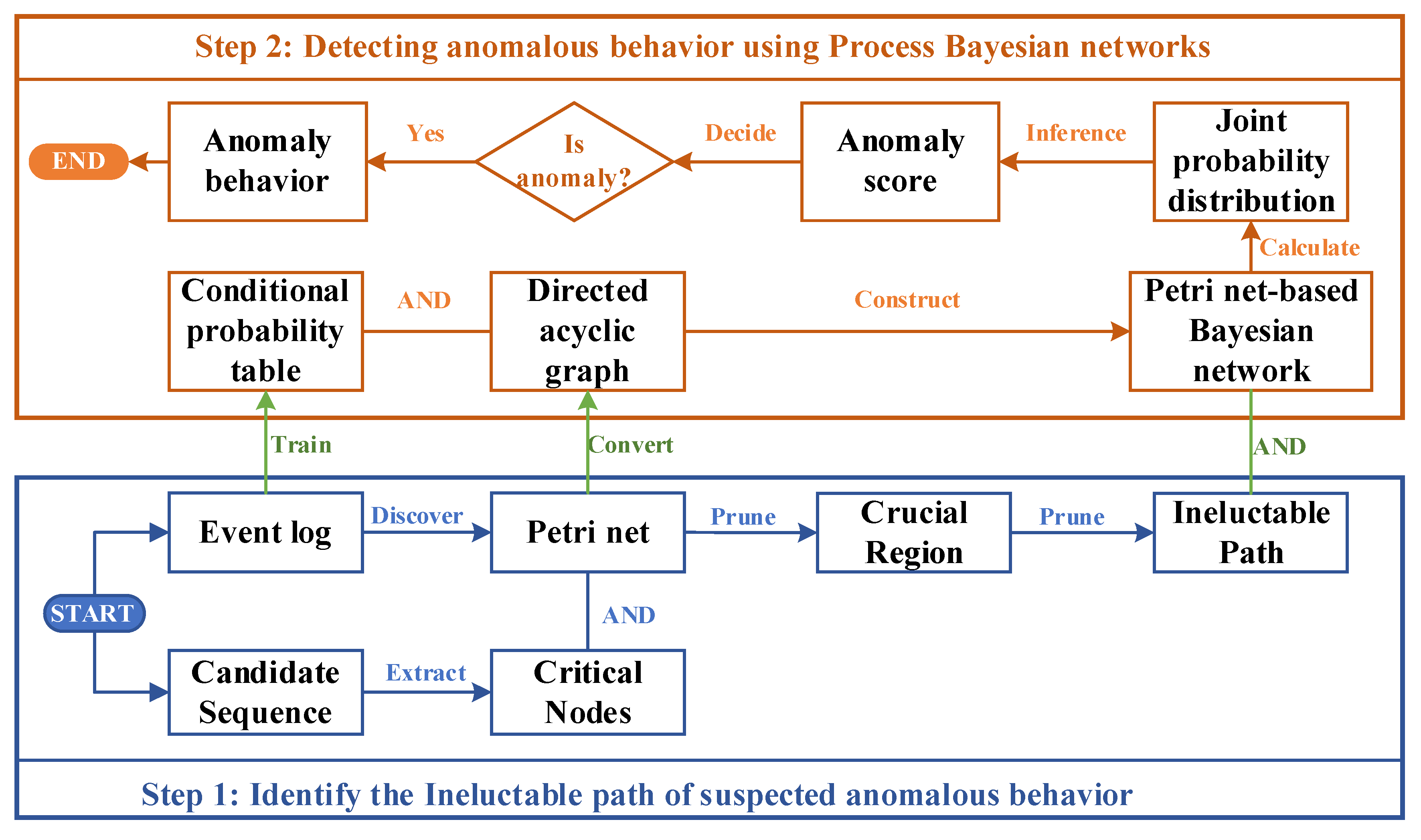
To address the above problems, this paper constructs a Petri net architecture-based Bayesian network PN-BBN from event logs to propose an algorithm to detect abnormal behavior from the perspective of behavior and data. The behavioral profiles analyze the behavioral relationships of activity contexts among business process activities. The Petri-based Bayesian network checks the probability distribution to determine whether the processes are normal or not, which mainly includes the following two steps, as shown in Figure 1.
(1) Determine the behavioral context using the behavioral profile. In this step, we locate the activity contexts of suspected anomalous activities at the behavior structure level, which are all on the same path. First, a business process model in the form of a Petri net is discovered from the event log using process mining techniques. Then, the critical node sets (the precursor and successor node sets) about the suspected anomalous activities are extracted from the candidate sequences. Further, the Petri net model is pruned based on the critical node sets to obtain the key regions. Finally, the behavioral profile of the process model is used to prune again to derive the ineluctable paths and thus obtain the behavioral context.
(2) Construct Petri Net-Based Bayesian Network for anomaly detection. The Petri net generated in step one is used as Bayesian network architecture, and the conditional probability table of the Bayesian network is learned from the event log, thus constructing a Petri Net-Based Bayesian Network. Based on this, the joint probability distribution values constituted by the nodes on this path are derived in combination with the critical path generated in step 1, and thus the anomaly scores are obtained. By comparing the anomaly score with the threshold value, it is possible to determine whether the current activity is abnormal behavior.
The model module most closely associated with the suspected anomalous activity is analyzed by constructing paths that necessarily contain the activity based on its behavioral characteristics. The decision is then based on the joint probability distribution of the cause (antecedent activity) and effect (subsequent activity) of the possible suspected abnormal activity. It considers the activity’s numerical fluctuation patterns and the business process’ behavioral impact.
The rest of the section is organized as follows. Section 2 briefly reviews the literature related to abnormal behavior detection. To facilitate the description of the core algorithm, the notations and concepts related to the Petri net model and Bayesian networks are introduced in Section 3. Based on this knowledge, we expand in detail the proposed Petri net architecture Bayesian network construction method and how it can be used for anomaly detection in Section 4. Additionally, the PN-BBN is implemented and validated using synthetic and real logs in Section 5. Finally, Section 6 summarizes the entire paper and indicates future research directions.
2. Related Work
Anomalous behavior detection has gained much attention. Regarding anomaly detection (also known as outlier detection and novelty detection) that exists in data mining, this class of methods ignores the dependencies of the system process activities. Therefore, only the problem of “anomalous behavior detection” in the field of process mining will be described in this section, and outlier detection beyond the relevant methods can be found in the literature for a detailed explanation [7].
Some studies consider anomalous behavior as deviant behavior in the process and thus use conformance-checking techniques to detect abnormal behavior in the system [8]. Such approaches use event logs as the object of analysis and mine a model by analyzing the events recorded in the logs. It is then compared with the initial or known reference model from which the unintended behavior is analyzed. Van Dongen et al. used integer linear programming techniques to implement Petri net-based alignment replay and thus computed the optimal alignment for consistency checking [9]. Nagy et al. integrated prefix-based alignment and multi-view checking techniques to achieve online conformance checking by analyzing the event stream and building a data Petri net [10]. A method based on the logarithmic novelty of the model metric was proposed to implement outlier analysis [11]. The event logs are first divided into reference and analysis data, and then a model structure is trained based on the reference data using semi-supervised learning. When the model parameters fit the expected range, it is used to analyze the anomaly scores of the data.
Considering the dramatic increase in the size of the log data recorded by information systems, Sani et al. considered that exact alignment is not always required, and they discarded the reference model and used the determined correct behavior to construct prefix trees to identify problematic activities by obtaining consistency values under the approximate method through edit distance [12]. To ensure the accuracy of this approximate alignment, Sani gave a method to quantify the maximum approximation error of an arbitrary sequence using edit distances that can guide the extraction of log subsets from logs to be extracted [13]. Some studies have directly used alignment techniques to analyze the variability of logs concerning the reference model. For example, a new fitness and accuracy metric was constructed, which obtains the differences between models and logs under the new metric using a divide-and-conquer strategy [14].
In some scenarios, exceptions are seen as traces of wrong behavior that are not beneficial to the business process, and such approaches focus on how to filter them out of the main path. Sequence mining techniques were used to detect and filter outliers from complex processes to improve the quality of event logs [15]. In real-time environments, earlier specifications were not always adapted to new scenarios. In this context, a class of methods for event stream analysis emerged. The literature [16] constructs an incrementally updated probabilistic automaton approach capable of performing a filtering analysis for each latest event, determining whether it is normal or not based on the probability distribution of that event while dynamically updating the probabilistic automaton. It removes all traces or sequences containing anomalies resulting in insufficient samples for analysis. Dixit et al. provided interactive operations that detect and fix misordered activities in event logs, thus improving log quality and ensuring sample adequacy [17].
The inability to provide a clear definition of anomaly structure is a challenge in anomaly detection. Nolle et al. used unsupervised learning to infer anomaly traces [18]. It introduces a self-encoder neural network that automatically completes the neural network’s learning process without labels to automatically analyze anomaly traces in the event log. Based on this, Krajsic et al. constructed a variational self-encoder network—a deep generative model based on regular training logs—and subsequently embedded it in an online environment for anomaly detection. Nolle et al. chose to construct an approximate process model from a deep learning perspective. It uses two recurrent neural networks that simulate the process structure from both front and back directions [19]. The logs were then aligned and analyzed with this network to detect anomalies and perform automatic corrections. Scholars such as Vertuam Neto provided an autonomous evolutionary online clustering algorithm called Autocloud [20]. It does not rely on a priori knowledge and can respond quickly while the system runs, significantly improving the algorithm’s efficiency.
Although some studies have analyzed abnormal behavior from a behavioral perspective, few studies have focused on the influence of this in the activity context. Therefore, we fuse the activity relationships of business processes and contextual joint probability distributions to construct Petri Net-Based Bayesian Networks that rely on behavioral relationships for abnormal behavior detection.
3. Background Knowledge
This section provides a formal description and illustration of the relevant definitions and notations of Petri nets and Bayesian networks used in the paper.
3.1. Petri Net Model
The starting point of this paper is the event log that records user operations and the system operation status in information systems. An event log consists of a set of traces . Each trace records the execution status of some activity of a business process under a particular case (i.e., event ). Each trace is a record of a single execution of the system.
A Petri net is a popular business process modeling language that uses circles (called places), boxes (called transitions), and arrows (called relation flow arcs) to model states, activities, and relationships in a process, defined and formalized as follows.
Definition 1
(1) denotes a finite set of places and denotes a finite set of transitions;
(2) ;
(3) .
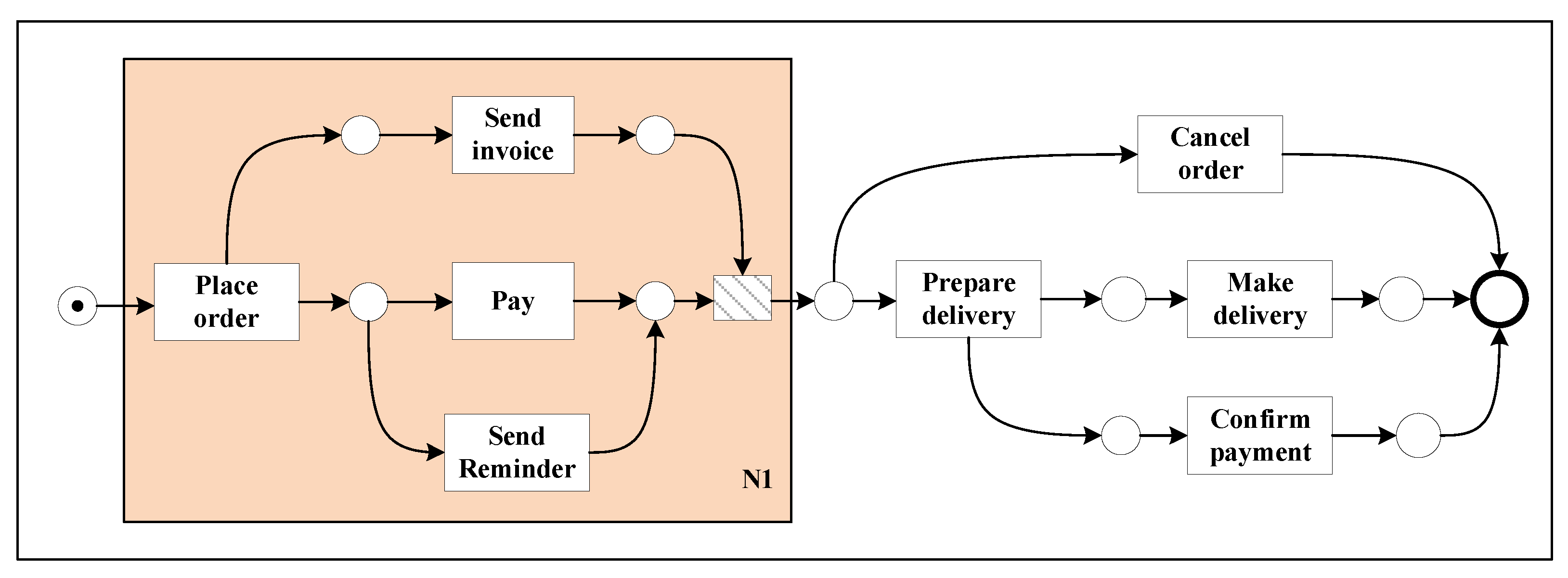
(2) states that there is no intersection between the range of the values of the place and the transition, and there is at least one place or transition in the net. (3) defines a relational flow arc as an arrow from place to transition or from transition to a place. Figure 2 gives a schematic diagram of the Petri net structure, where the leftmost circle is the starting place. Furthermore, the black dot in the middle of the place is the marker by which the transfer in the Petri net can formally describe the occurrence rule of this net structure.
Definition 2
Given a Petri net. For, writeas the preset or input set of, andas the post-set or output set of.
Process discovery techniques discover a business process model described by a Petri net from an event log. Next, a correspondence is established between the events recorded in the event log and the activities represented by the transition in the model using a projection function.
Definition 3
(Projection).Given a process model m, an event log L, and an activity A in L, the corresponding model variation in activity A is noted as:
When only one event in the sequence is considered, its projection is denoted as:
We introduce the definition of the behavioral profile to capture the relationship between the process activities in the behavioral structure.
Definition 4
((Behavioral Profile) [22]).Given a process modeland two activities. If there exists a trace, thenis said to be a weakly sequential relation, denoted. Then, any pair of activitiesin the model satisfies one of the following three relations:
(1) The strict order relation: , if ;
(2) The exclusiveness order relation: , if ;
(3) The interleaving order relation: x||y, if .
3.2. Bayesian Networks
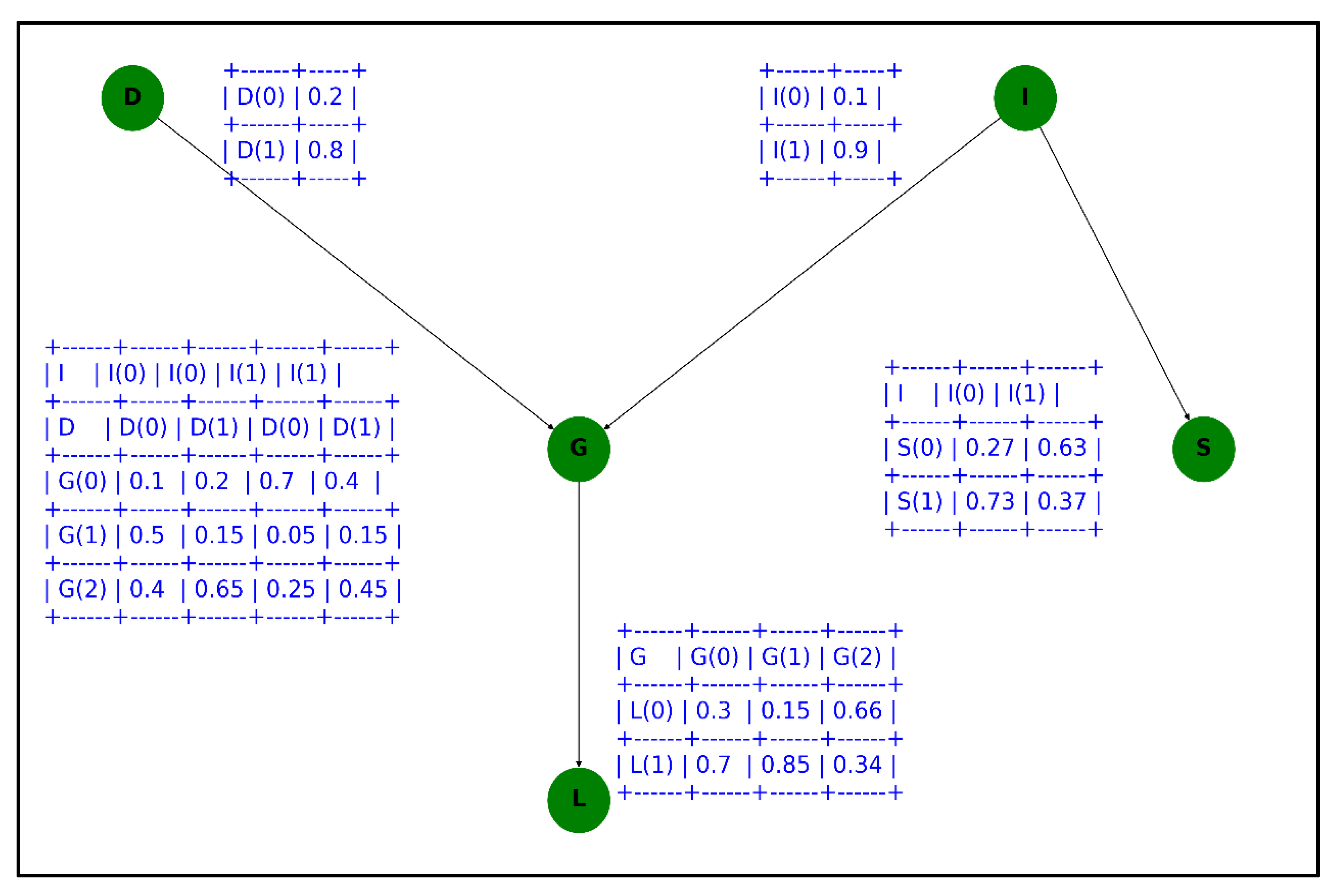
When the random variables are strongly correlated, Bayesian networks [23] can effectively describe their interactions, as shown in Figure 3. Based on the random variables and their causal relationships, we formalize the Bayesian network as follows.
Definition 5
(Bayesian Network).A Bayesian network consists of a directed acyclic graph G and a setof conditional probability tables, where the graph nodes are described using circular notation and represent a set of random variables. Arrows connect the nodes, indicating the existence of conditional dependencies between two nodesand.
When the variables are significant, the association between them is complex, and in this case, it is almost impossible to model the joint probability of the variables for analysis. Bayesian networks are set up with independent assumption rules to reduce the number of parameters involved. Local independence among nodes in a Bayesian network is considered, and a node is conditionally independent of all non-predecessor nodes when the predecessor node of that node is known. Using to denote the set of parents of the variable , the local conditional probability distribution of is marked as . The product of the local conditional probabilities of each forms the joint probability distribution of , denoted as .
The global independent relationship between nodes is discussed in two cases: (1) nodes are directly connected, and (2) nodes are indirectly connected. In case (1), as in Figure 3, “D and G,” “I and S,” etc., the two nodes are directly connected. In this case, the node relationship is a direct causality, and there are only two ways to connect the two, so any change in one variable will affect the other, i.e., the two nodes are unconditionally independent. In case (2), the two nodes are connected via a third node, at which point there are four types of connections corresponding to four relationships.
① Indirect causality: as in Figure 3, for nodes D, G, and L, if G is known, then D and I are conditionally independent, noted as ;
② Indirect causal relationship: as in Figure 3, for the nodes L, G, and I, if is known, then and are conditionally independent and are denoted as ;
③ Co-causal relationship: as in Figure 3, G, S, and I are nodes. If is known, then and are conditionally independent, denoted as ;
④ Co-result relationships: as in Figure 3, D, I, and G are nodes. If is unknown, then and are conditionally independent, noted as .
The probabilistic inference problem for Bayesian networks is defined as follows, where the conditional probability of some subset is computed based on the above Bayesian network and its properties in the presence of known partial variables .
4. Detecting Abnormal Behavior using Petri Net-Based Bayesian Network
In this section, we describe in detail how to construct a Petri Net-Based Bayesian Network from event logs and then detect abnormal behaviors in the business by probabilistic inference, which consists of two main phases. In the first phase, the critical paths to the suspected abnormal behavior are constructed based on the business process model to consider the impact of the activity context from a behavioral perspective, the details of which are described in Section 4.1. In Section 4.2, we introduce the second phase of the algorithm. By introducing Bayesian network inference techniques, we calculate the conditional probability of occurrence of the suspected abnormal behavior based on the business process structure, thus enabling the detection of abnormal behavior under business logic constraints.
4.1. Using Behavior Profiles to Determine Behavior Context
We use the business process model as the skeleton of the Bayesian network, i.e., the DAG structure in the Bayesian network is replaced by the business process model. This strategy aims to analyze the impact of activity contexts in different process structures from a fine-grained level. It is first necessary to construct process models that capture the behavioral structure of business activities. We use an advanced process discovery method (Split Miner) [24] to mine Petri net representations of business process models from event logs. It can discover business processes’ sequential, concurrent, and selective structures from complex logs. Moreover, the method can balance accuracy and simplicity, resulting in understandable and high-quality models.
For activities in the model, the activity on the select branch cannot appear in the same case as the path where the activity is located. In contrast, the activity on the concurrent branch can appear in its context. Therefore, activities on concurrent and selective branch paths have different degrees of influence on the suspected abnormal activity in the current analysis throughout the business process. Activities on concurrent and sequential branches should receive more attention than activities on selective branches.
Next, we limit the analysis to the crucial regions of suspected abnormal behavior in the model to focus on the events that directly affect abnormal activity. The crucial regions of suspected anomalous activity were designated as subnetworks of the model.
Definition 6
(Crucial Region).Given a Petri network, the crucial region (CR) is a subnet of the Petri network, i.e.,
where the starting node of the crucial region is defined as place, subject to one of the following two conditions:
(1) ;
(2) .
The end node of the crucial region is defined as the place , subject to one of the following two conditions:
(1) ;
(2) .
For example, the subnet in Figure 2 is a crucial region. This crucial region’s starting and ending nodes are and “end”, respectively.
Thus, determining the crucial area depends on the start and end nodes. Next, we give two additional definitions based on Definition 2, which locate the process activities’ start and end nodes in the model structure.
Definition 7
(Predecessor and successor activities).Given an activity, its predecessor activity is denoted as, and its successor activity as.
Further, we define the activity’s predecessor and successor gateway to identify the XOR gateway.
Definition 8
(Precursor and successor gateways).Given an activity, its precursor gateway is denoted as, and its successor gateway is denoted as.
The gateway and its determination condition are defined as .
The gateway and its decision condition are defined as .
As mentioned above, the algorithm in this section aims to find an ineluctable path from the business process model that contains the suspected anomalous behavior, which will be denoted as an ineluctable path, formalized as follows.
Definition 9
(Ineluctable Path).Given a set of sequences CS containing suspected abnormal behavior x and the critical region CR in which they are located, the ineluctable path IP concerningis defined as:
We define the nodes on this path as the behavioral context of the business process activity.
Based on the definition mentioned in the previous section, we formalize the ineluctable path identification method for anomalous activities in Algorithm 1. The algorithm uses event logs to research a set of candidate activity sequences containing suspected anomalous behavior. Finally, it obtains a critical path with suspected abnormal activity as the core.
| Algorithm 1: Ineluctable Path Identification. |
 |
At the beginning of the algorithm, Algorithm 1:2 initializes a variable for storing suspected exception events. As the basis of this phase, the business process model is generated by the advanced Split Miner method (Algorithm 1:3). The first and last events of each candidate sequence are extracted using ‘i’ and ‘e’, respectively (Algorithm 1:4–5). Furthermore, their projected activities (transitions) in the model are noted as and (Algorithm 1:6). The use of and to initialize the starting and ending activities are intended to reduce the search space since it narrows the gap between the region formed by the sequence of the selected activities and the critical region. Algorithm 1:7–29 implements the same search strategy for each activity in the candidate sequence (excluding the first and last). The key regions corresponding to the candidate activity sequences in the model are first identified. In contrast to the proposed definition section, the analysis process requires first determining the boundaries of the key regions, i.e., the starting and ending nodes of the key regions. We analyze all suspected anomalous activities in the candidate activity sequences one by one (Algorithm 1:7).
Algorithm 1:8 starts traversing the projected variants of the starting activity on the model in the candidate activity sequence. If the predecessor activity of a transition is empty, the transition is the first activity of the model. Then, the input place of the transition is one of the starting activities of the critical region, which is kept in the original set. Moreover, the analysis of the following starting activity is started (Algorithm 1:9–10). Otherwise, it is further determined whether the predecessor gateway of the transition is (Algorithm 1:11). If not, the transition is removed from the starting activity set (Algorithm 1:12). Subsequently, the analyzed object is replaced with its predecessor activity. The search is iterated until the predecessor gateway is satisfied or the predecessor activity is empty (Algorithm 1:13). After that, the analysis proceeds to the next starting activity (Algorithm 1:14). When Algorithm 1:8–16 are finished, the set of starting activities for the critical region is available.
Next, a similar search approach (Algorithm 1:17–24) is taken for the projection transition of the terminated activity on the model in the candidate activity sequence, with the difference that the search direction is reversed. We start with the projected terminated activity on the model in the candidate activity sequence and search backward until we find the xor gateway or the last activity of the model. When Algorithm 1:17–24 are completed, the set of terminating activities in the critical region is available.
The starting and ending activity sets obtained from the previous steps define the critical region (Algorithm 1:25). For the suspected anomalous activity x in the candidate sequence, its projection in the model is noted as x’ (Algorithm 1:26). Finally, we approximate the key region nodes based on the behavioral profile knowledge and remove the nodes on the XOR branch (Algorithm 1:27). That is, we keep the nodes that are in strict and cross-order with x’, and remove the nodes and dependencies that are in exclusive order. At this point, Algorithm 1 ends, and we obtain a path that contains the suspected anomalous activity being analyzed, and all the nodes on this path are closely related to this node. In addition, we output the generated process model to provide the structural basis for training the Bayesian network in the next stage.
4.2. Constructing Petri Net-Based Bayesian Networks for Anomaly Detection
We construct a Bayesian network of fusion processes based on event logs in this stage. The Bayesian network consists of two parts: a directed acyclic graph and a conditional probability table, so the construction process is naturally divided into two steps.
(1) Determining the inter-activity topology.
(2) Learning conditional probability table.
In step (1), we transform the labeled transitions of the activity in the place and corresponding logs of Petri nets directly into directed acyclic graphs.
Example 1.
As shown in the Petri net subnet above in Figure 4, there are two transitions, with a and b in the figure. We perform the transformation from left to right. The first node is place. The second node is a transition a, and are both places, while , and at this point, it needs to be converted. Let , while setting to empty, as shown in Figure 4, the connection between a and b has been established. Subsequently, node b is analyzed. is a place, and is empty, so is set to empty to obtain Figure 4. The Petri net subnet in the example has been converted to the corresponding directed acyclic graph.
However, most process models do not have this simple structure, and the conversion process faces two main challenges.
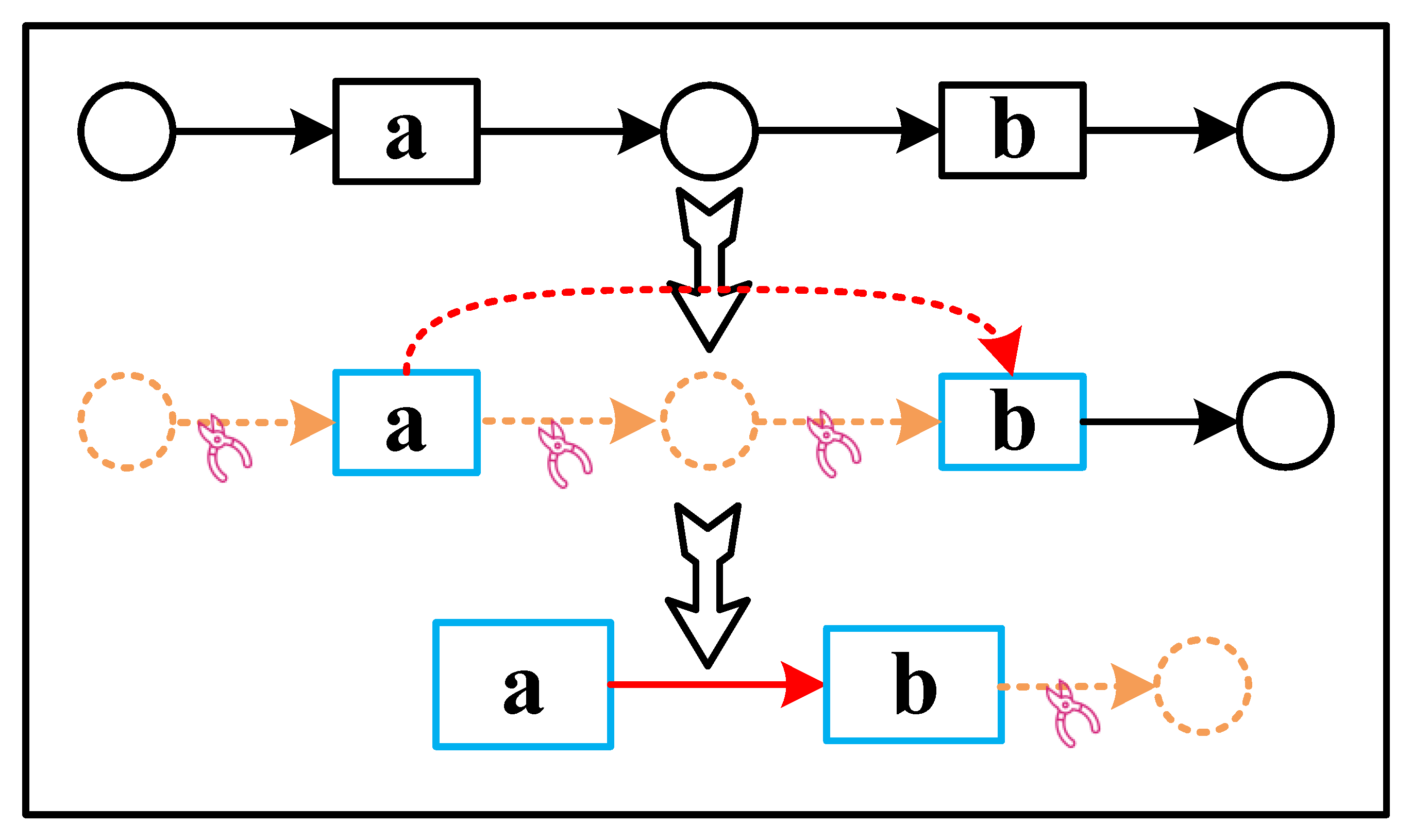
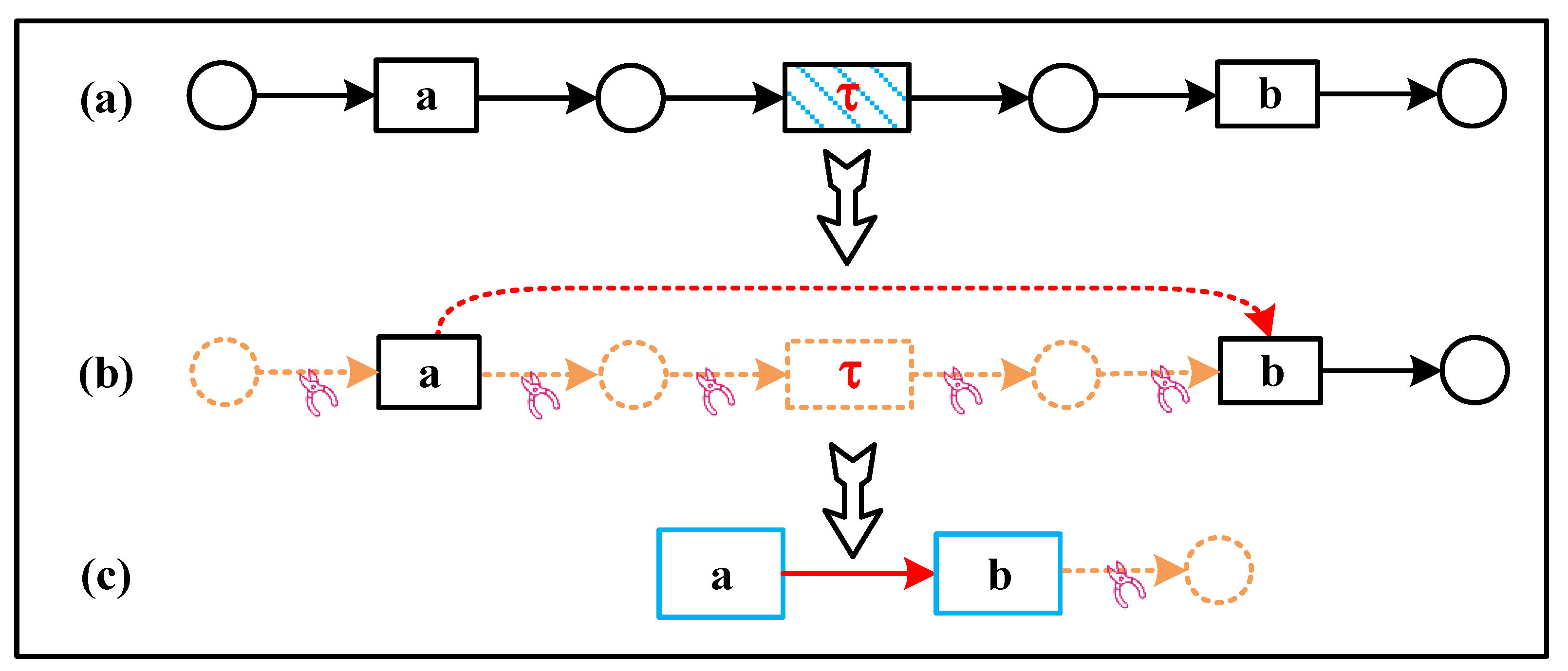
The invisible transitions problem: The Petri net model can model the selection, concurrency, and cyclic structure of system activities using place and transitions, but the ability to express the process model drawn by relying only on the transitions activities provided in the logs is limited. To improve the fitness of Petri nets, hidden transitions are introduced in the process discovery algorithm to enhance the routing capability. These invisible transitions are activities that do not exist in the logs; therefore, we remove the invisible transitions that are strictly sequentially connected to the labeled transitions in the Petri net. Again, we use an example for an explanation.
Example 2.
As shown in Figure 5, the difference with Example 1 is (Figure 5a); skip this invisible transition and continue to observe the next one. At this point let , i.e., the transition a is directly connected to b (Figure 5b). Repeat the above example to obtain the result after the transformation (Figure 5c).
Loop problem: Early process discovery algorithms rarely considered the loop structure in the system process when mining the process model from the event log [25]. However, with continuous research, scholars found that the actual operation of the system is accompanied by a variety of complex structures, such as loops and concurrency. The correct mining of these structures is beneficial to improve the accuracy of the system description, so most of the current advanced process discoveries make the cyclic structure a focus of analysis. Furthermore, the topology of the Bayesian network is a directed acyclic graph, so a key problem in constructing a Bayesian network based on the Petri net is to transform the Petri net’s cyclic structure into a directed one acyclic structure.
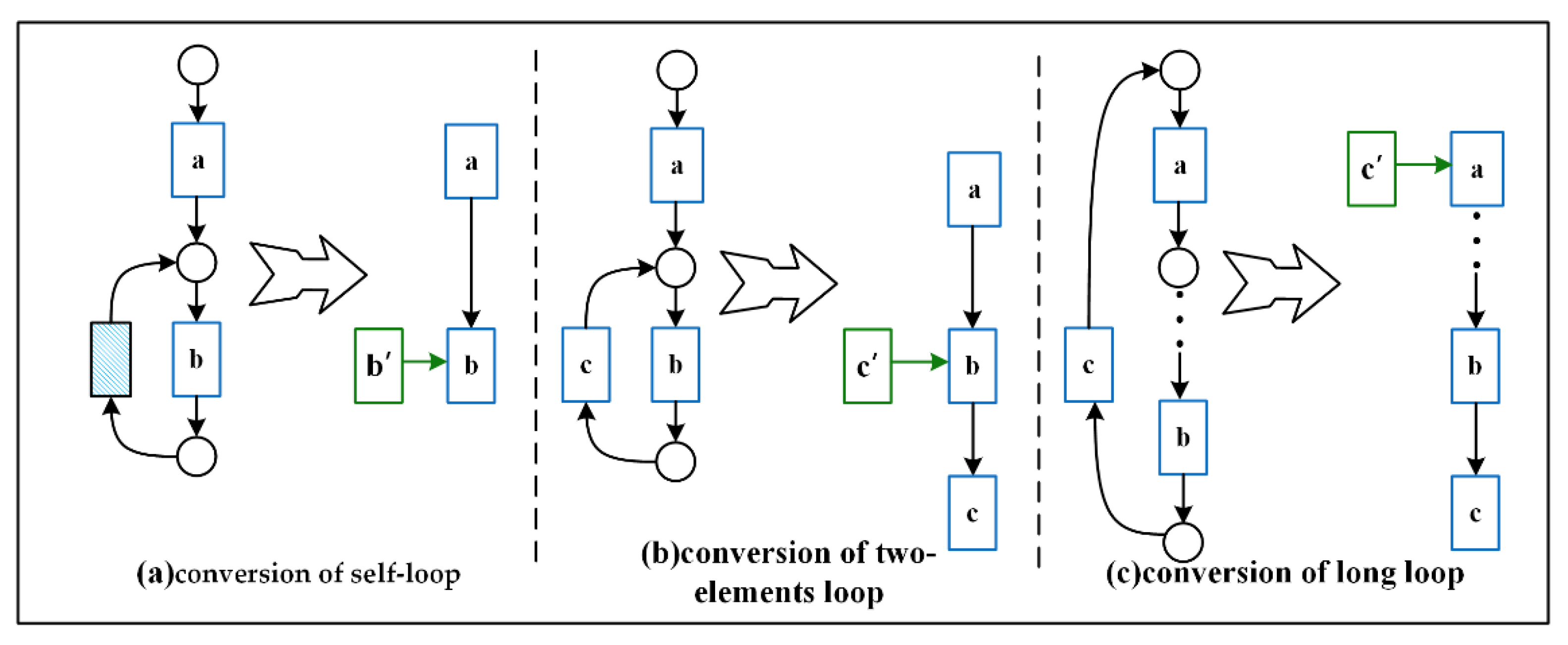
We were inspired by Prasidis et al. [26] to create a copy of the last activity of the loop body to disassemble the loop and form a new sequence structure, as shown in Figure 6.
① Self-loop: The loop contains only one transition (only tagged variation is considered), as shown in Figure 6a. The predecessor transition (non-hidden variation) and the successor transition (non-hidden transition) of activity b are both b. We introduce a new label b’, which transforms the Petri net structure on the left side into the structure on the right side.
② Two-elements loop: The loop is shown in Figure 6b when it contains two transitions. We introduce the new label c’, thus disassembling the first-order loop into an acyclic structure.
③ Long loop: Figure 6c shows when loops contain more than one transition. Similarly, we take the last element of the loop body and introduce its copy token c’ to disassemble the loop structure.
The currently obtained ineluctable paths perform a pruning operation on the process model, i.e., they approximate the periphery of the critical region and the XOR branch of the suspected anomalous activity. The ineluctable paths regarding the suspected abnormal behavior x still contain complex branching structures, as shown in Figure 4. We assign corresponding weights to the different structures based on the behavior profile and Bayesian network knowledge.
Definition 10
(Weight function).Given a suspected abnormal activity and the ineluctable path (I)P in which it is located, use the weight functionto assign a value to the weight of each node on the path:
where the node is all nodes in the IP,refers to the number of libraries from activity to activity, and |XOR| describes the number of XOR structures from activityto activity. The fractions on the right side of this expression form a penalty factor: as the XOR structure in the IP increases, the penalty factor increases; asin the node increases, the penalty factor also becomes more extensive. We use the weight function to define the difference between the activity penalty factor and one as its weight.
The Bayesian network inference idea enables us to infer the distribution of activities from the process model in conjunction with the business logic in which the activities are located. For example, inferring the result based on the cause of the activity, inferring the cause back from the results of the available observations, and reasoning from a mixture of partial causes and results. For suspected abnormal behavior, the conditional probabilities of other nodes in the IP are combined with the process structure characteristics for inference analysis. We formalize the inference process as Algorithm 2.
| Algorithm 2: Anomalous behavior detection leveraging probabilistic inference. |
 |
Algorithm 2 is a further analysis based on Algorithm 1, and thus the input of this algorithm is derived from the output of Algorithm 1. We input the event log again to calculate the conditional probability table of the Bayesian network. In addition, anomaly threshold O needs to be input to provide judgment information (Algorithm 2:Input). Anomalous behavior detection is performed using the function detectAnomalyBehavior (Algorithm 2:1–9). First, we initialize a list structure for storing the activity relations of the directed acyclic graph (Algorithm 2:2).
Next, based on the methodology proposed above, we construct the Bayesian network topology from the Petri net model, i.e., a directed acyclic graph with the business process model as the skeleton (Algorithm 2:3). The specific construction process is shown in the function BuildPN-BBN (Algorithm 2:10–32). In this function, the discriminative order of Kusho, hidden variation, first-order cycle, second-order cycle, multi-order cycle, and directed acyclic relation pairs is processed in analogy with Example 1 and Example 2. At the end of the function, a list of the relation pairs of the directed acyclic graph structure, i.e., the network skeleton, is obtained.
Subsequently, we trained conditional probability tables (Algorithm 2:4) using event logs as data samples to capture inter-activity structural dependency information. The specific training steps are beyond the scope of this paper and can be found in the literature [23] for detailed support.
Next, we obtained an anomaly score by Bayesian network inference (Algorithm 2:5). Since the degree of association between activities on different branches of the behavioral profile varies, to distinguish between distance differences and structural differences, we define a weight assignment method and a joint probability calculation method in the inference function inference (Algorithm 2:33–39). Based on the cause and effect of the activity and the mixed inference, we obtain a probability value under contextual constraints. It is compared with the anomaly threshold, and if it is higher than the expected threshold, it can be determined as anomalous behavior based on the business behavior relationship (Algorithm 2:6–8).
5. Evaluation
This section describes the event logs, assessment metrics, experimental procedures, and results used for the evaluation.
5.1. Event Log
We use the open source datasets commonly used in process mining research for evaluation.
Receipt (CoSeLoG project: Receipt phase of an environmental permit application process (WABO), CoSeLoG project http://data.3tu.nl/repository/uuid (accessed on 8 September 2022): a07386a5-7be3 -4367-9535-70bcge77dbe6): This log is derived from the BPI Challenge and is often abbreviated as Receipt.
This dataset records the activities and processes of a city (anonymized) at each stage of the environmental permit application process.
Sepsis (Mannhardt, Felix (2016): Sepsis Cases—Event Log. 4TU.ResearchData. Dataset. https://doi.org/10.4121/uuid:915d2bfb-7e84-49ad-a286-dc35f063a460 (accessed on 8 September 2022)): This log comes from the 4TU open-source data platform. It records the treatment flow of patients with Sepsis conditions, including events such as emergency room, hospitalization, discharge, and other execution information (e.g., time stamps).
In addition to the two logs mentioned above, we injected/removed random events of varying degrees on top of the Receipt and Sepsis logs to simulate anomalous behavior. When the amount of noise in a log trace is exceptionally high, analyzing the trace is no longer meaningful, so we set the maximum injection percentage to 25%. In addition, we mainly focus on exceptions caused by unintended execution orders of events, so more attention is put on injecting events rather than deleting them.
Therefore, we used 16 logs to test, and the statistics of the logs are shown in Table 1.
5.2. Evaluation Indicators
The proposed method is evaluated in three main aspects.
(1) Whether the abnormal behavior can be correctly identified.
Recall: The ability of the algorithm to identify abnormal behavior is judged by measuring the anomalous behavior identified correctly. The Recall is the ratio of correctly identified anomalous behaviors (True positive) to the number of inserted abnormal behaviors. The resulting value is a decimal number between 0 and 1. When the value is close to one, the abnormal behavior is almost entirely correctly identified.
(2) Whether the model quality can be improved.
To measure the change in model quality, we use the metrics fitness and simplicity, commonly used in the process mining domain.
Fitness: A token-based replay method calculates the percentage of traces that can fit the model and measures how well the model fits the traces. By calculating the fitness value, we can quantify the model’s expressiveness before and after the anomalous behavior identification and thus make a numerical comparison (the fitness value is between 0 and 1). When the value is close to one, the model can reflect the log behavior well.
Simplicity: We analyze the effectiveness of abnormal behavior detection by measuring the model’s simplicity. It is defined formally in the following equation.
The mean degree of both the library and the transition is calculated based on the input degree (the number of input arcs) and the output degree (the number of output arcs). The number k is a value somewhere between 0 and infinity. And simplicity is a value between 0 and 1. The more the value approaches one, the simpler the model is.
(3) Whether it can be executed efficiently.
To analyze the temporal variability of our approach with other algorithms, we will compare the running time of different algorithms (Duration = data importing + structure learning + probabilistic inference). In this metric, we need to consider the time of various phases of the algorithm, including the time required for data preprocessing, model construction, and detection of abnormal activities.
5.3. Bayesian Structural Analysis
In this subsection, we use Sepsis logs to show in detail the exact implementation of the algorithm.
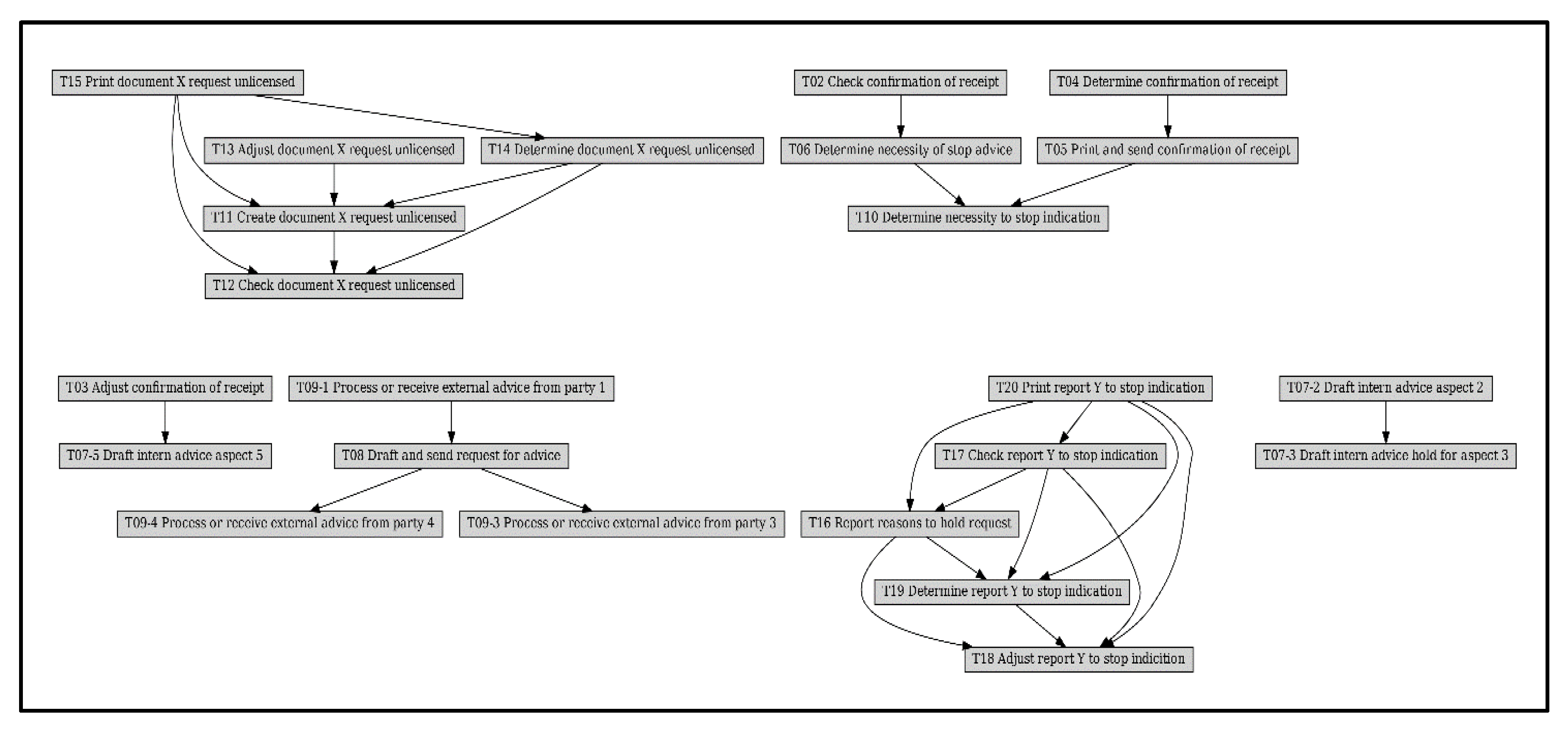
Figure 7 shows the process models mined from Sepsis logs using Split Miner (https://apromore.com/research-lab/ (accessed on 8 September 2022)), which can obtain simplistic and accurate business process models from complex event logs. Compared to Inductive Miner, another advanced process discovery method, Split Miner is slightly less suitable for obtaining models. However, the latter comes at the expense of an accurate description of the model, i.e., the model is more likely to have behavior structures that do not exist in the logs. Therefore, we use the more balanced SM method.
We illustrate this with an example of a partial log sequence in a synthetic log. Given a candidate sequence,
we first determine its starting event set as:
In this case, the candidate sequence is projected in the model with a starting event set and a projected ending event set .
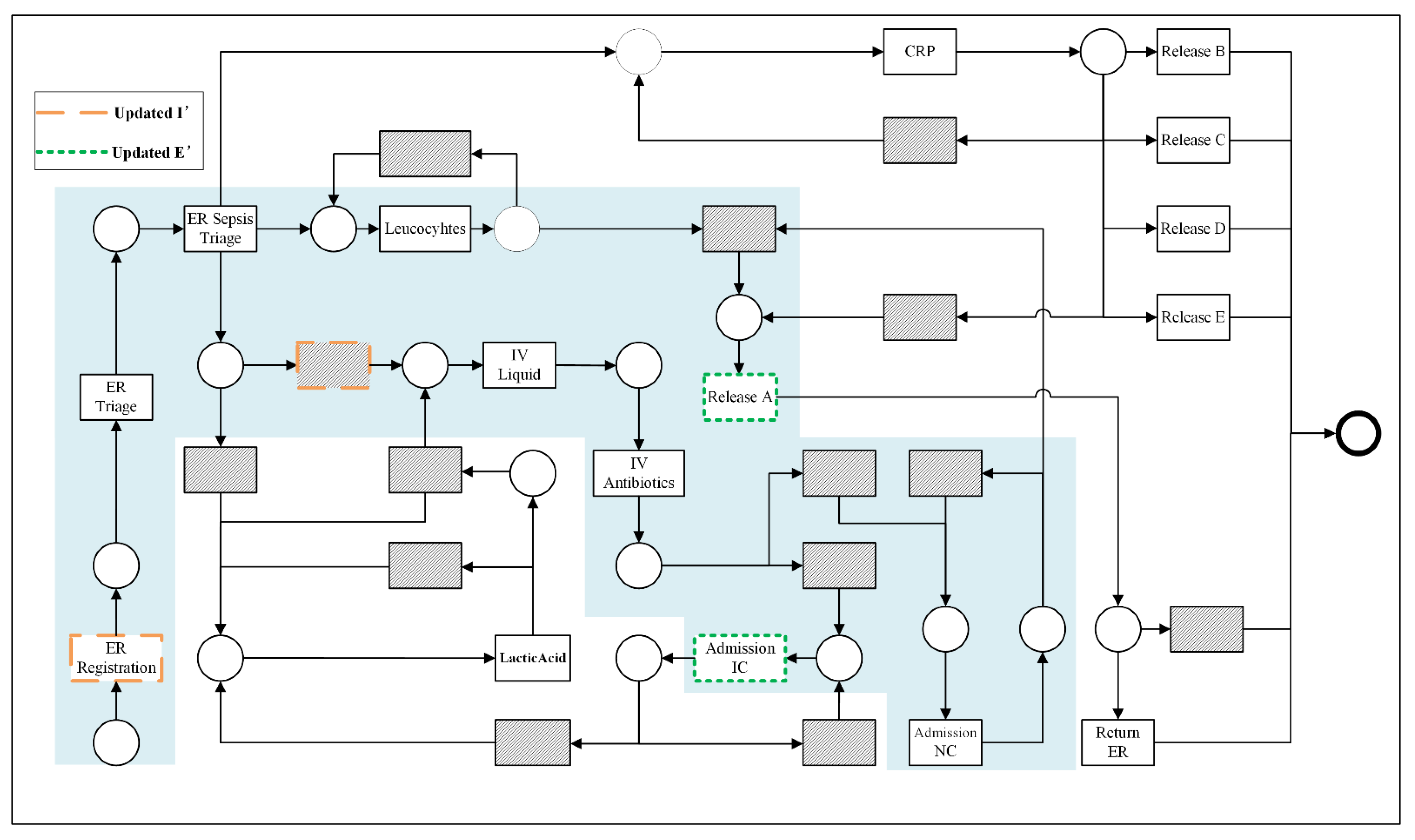
Subsequently, the elements in are filtered and updated based on Algorithm 1 to obtain the updated set of projections . The implicit transition is an activity that appears only in the model and not in the log; it is used for routing roles and has no execution semantics. The updated projected activity set and the critical regions defined by it are shown in Figure 8. We performed the first reduction in the original Petri net model by projecting the starting and ending activity sets, excluding the model structure at the periphery of this set and keeping only the critical regions.
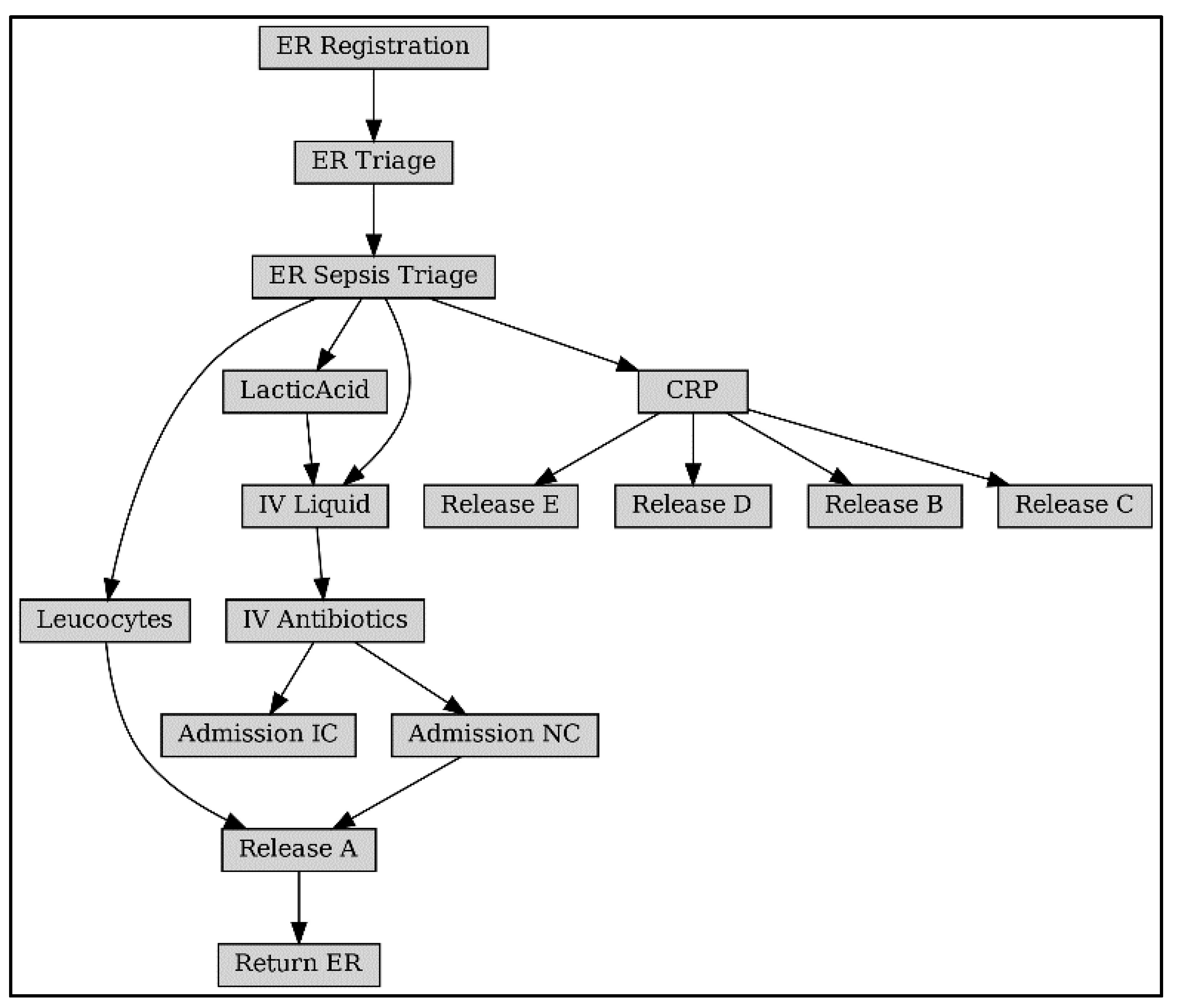
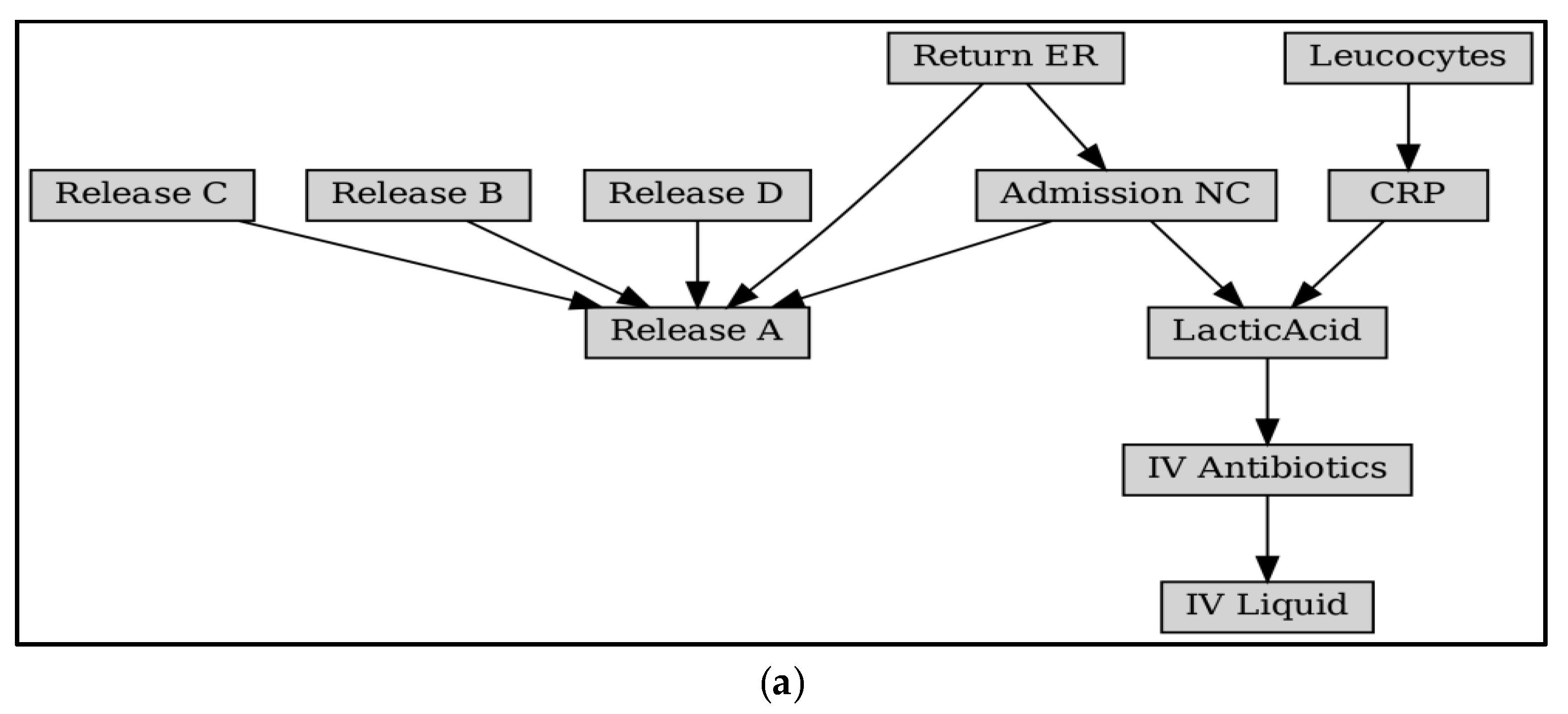
Figure 9 shows the model fragment obtained after the second reduction, i.e., the ineluctable paths. After the two drops, we focused the analysis on the paths most closely related to the behavior of activity X to be analyzed. At this point, the ineluctable paths are all directly or indirectly related to X. These nodes can appear in the same path (e.g., ER Registration, IV Liquid, and Leucocytes, when interpreted in terms of behavioral profile relations, the latter two can be obtained as concurrent activities of the former, and therefore the three activities are co-occurring in the log).
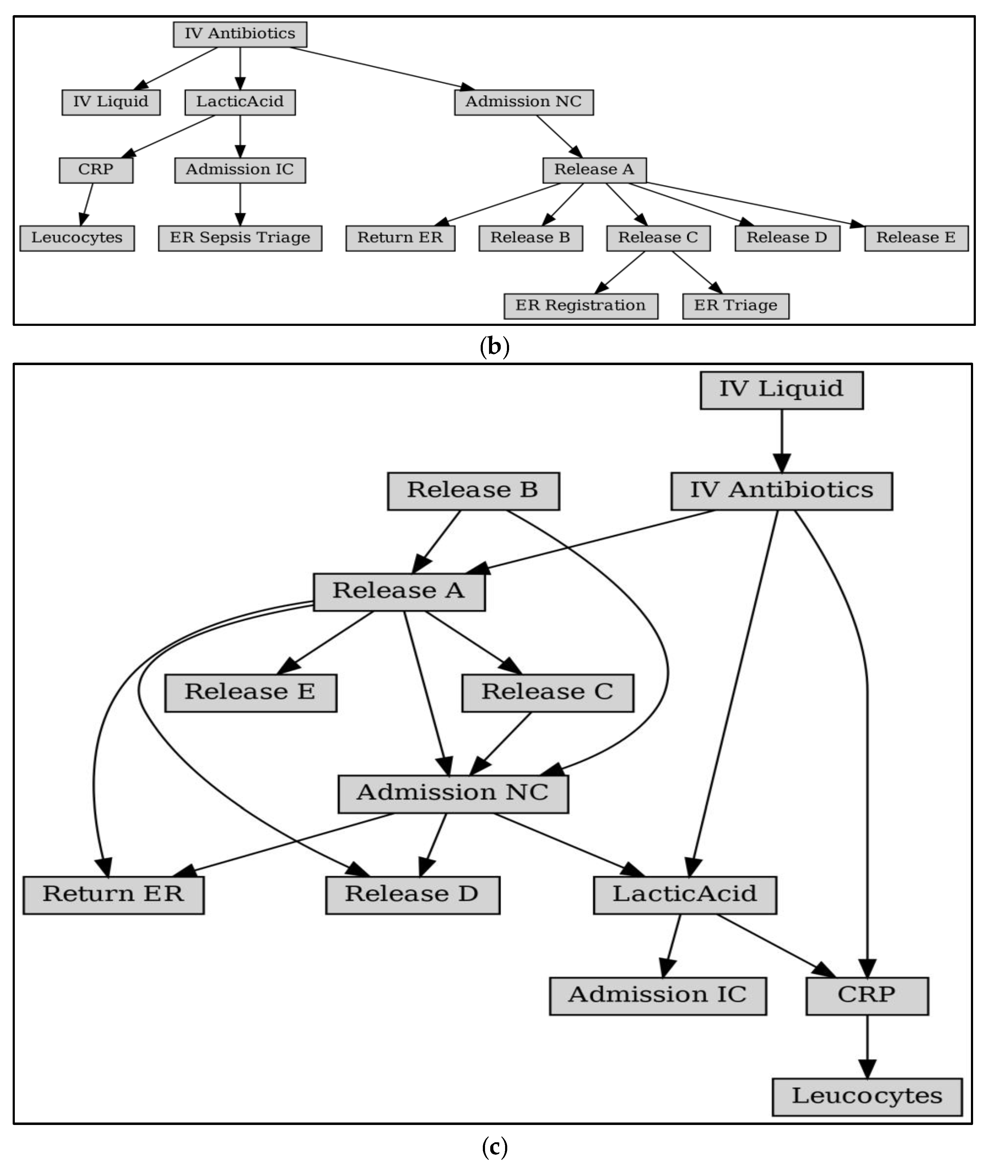
Figure 10 shows the Bayesian process network with the Petri net model as a framework. As a comparison, Bayesian network structures obtained using traditional structure learning methods are given, such as the Constraint-Based Learning algorithm in Figure 11a, the Tree Search algorithm in Figure 11b, and the Hill Climb Search algorithm in Figure 11c [28]. Analysis of the network structure reveals that it is challenging to obtain the correct structure of the business process model with Bayesian structure learning methods:
(1) The number of activities is incomplete. As can be obtained from Table 1, Sepsis logs contain 16 activities; PN-BBN obtains 16 activities; and the number of activities obtained by the structural learning method is 11, 16, and 13.
(2) The activity dependency is not accurate. For example, the starting activity of the business is ER Registration, and the corresponding direct dependency is (ER Registration, ER Triage), which is not reflected in any of the three models in Figure 11.
(3) Parameter accuracy. Since the parameter learning of Bayesian networks is trained based on the network structure, it can be inferred that an inaccurate network structure will inevitably lead to inaccurate results of parameter learning.
5.4. Anomaly Detection Results
We analyzed the performance of anomaly detection using the four metrics proposed in this section, and we plotted the experimental results under different settings in Table 2. Two original logs that did not contain anomalous sequences were considered control groups, and the derived data from the two logs were analyzed separately. Therefore, the Receipt and Sepsis rows did not have the results about Recall and the results of using the four algorithms BN by Constraint-Based Learning, BN by Tree Search, BN by Hill Climb Search, and BN by Petri-based Learning to eliminate the abnormal. The fitness and simplicity values were obtained after the values were removed, and we recorded the results generated by the logs without operations as a None column to compare the degree of improvement in log quality before and after the analysis.
The top half of the data in Table 2 shows that the Petri-based Bayesian network always obtained the highest values in the experiments on Receipt logs, which is consistent with the intuitive understanding of the Bayesian structure (Figure 10 and Figure 11). This is because this paper’s anomalous behavior detection assessment metric is inclined to be a behavior-level metric. Therefore, the three methods, BN by Constraint-Based Learning, BN by Tree Search, and BN by Hill Climb Search, presented lower levels overall due to their misrepresentation of the behavioral relationships, which led to their inability to identify behavioral biases. After several tests, it was found that these three had no obvious pattern in the result values regarding the fitness and simplicity metrics of the behavioral perspective. The following highest values of each metric were randomly generated among these three. In addition, the Recall values of each group of logs in Table 2 revealed that the Petri-based Bayesian network can effectively identify the injected anomalous behaviors. When injected anomalies are higher, the Recall value is lower, the fitness is smaller, and the simplicity decreases. That is, the recognition of abnormal behaviors decreases, the quality of logs decreases, and the complexity of the model structure increases.
The data in the lower half of Table 2 show the experimental results for the Sepsis series of logs. The data showed that the Constraint-Based Learning algorithm, in this case, could hardly provide suggestions for anomaly detection. We further examined its generated Bayesian network structure, as shown in Figure 12. The network structure was modeled as six independent network segments, which had a large gap with the actual process relationship, thus affecting the quality of its results. Meanwhile, the Petri-based Bayesian network produced new logs that outperformed the original event logs, significantly reducing the impact of abnormal behavior. Bn by Tree Search and bn by Hill Climb Search showed results that were not considered regular, both performed by providing sub-high values.
Finally, we analyzed the running times of the different algorithms. The algorithms compared in this section all had a good performance on the event logs, and the injection of different percentages of noise had little effect on the running speed, so we enumerated the running times in both logs as positive and negative errors after several experiments as follows.
BN by Constraint-Based Learning:
BN by Tree Search:
BN by Hill Climb Search:
BN by Petri-based Learning:
The above running times show that the proposed Petri-based Learning had a clear advantage in constructing the Bayesian structure. In contrast, the other three Bayesian network structure learning methods took a long time in this stage.
6. Summary
To improve the accuracy of the network’s representation of process behavior, we propose a Petri Net-Based Bayesian Network for abnormal behavior detection. To improve the accuracy of the network’s description of process behaviors, we formalized the behavioral relationships as process models and used them as the architecture of the Bayesian network. Advanced process model discovery techniques guarantee the model fitting ability to analyze the behavioral relationships between activities effectively. Using behavioral contours to approximate the analysis space allows the algorithm to focus on the causes of the triggering of abnormal behaviors and the effects of the results on them, which helps to improve the efficiency and accuracy of the algorithm. The comparative experiments with synthetic and real case data showed that the Bayesian process network proposed in this paper, which considers behavioral and probabilistic relationships among activities, had better results.
In addition, the Bayesian process network uses event logs as the object of analysis and a process model in Petri nets as the architecture. Therefore, the process is not limited by the process discovery algorithm and can be hot swappable and replaced with the current state-of-the-art process discovery algorithm to guarantee the accurate description of business activities and the adaptability of the algorithm to different scenarios. Moreover, based on the inference of joint probability distributions among activities for anomaly detection, it reduces the requirement of domain knowledge to a certain extent. It facilitates the better identification of anomalous behaviors by non-specialists.
However, offline data analysis is limited by policies and technologies, such as damaged, lost, or no access to data. Therefore, further research will obtain insights about online scenarios by analyzing event streams while the system runs.
Author Contributions
K.L.: conceptualization; methodology; software; writing—original draft; and visualization. X.F.: funding acquisition and writing—review and editing. N.F.: methodology; writing—review and editing; and investigation. All authors have read and agreed to the published version of the manuscript.
Funding
This research was supported by the National Natural Science Foundation, China (Nos. 61572035, 61402011), Key Research and Development Program of Anhui Province (2022a05020005), the Leading Backbone Talent Project in Anhui Province, China (12 January 2020), and the Open Project Program of the Key Laboratory of Embedded System and Service Computing of the Ministry of Education (No. ESSCKF2021-05).
Data Availability Statement
All the data in this paper were obtained from https://data.4tu.nl (accessed on 8 September 2022). Additionally, the algorithms were implemented based on PM4Py and PMGPY. Experimental data and code related to this paper can be obtained by contacting the corresponding author.
Conflicts of Interest
The authors declare no conflict of interest.
References
- Bezerra, F.; Wainer, J.; van der Aalst, W.M.P. “Anomaly Detection Using Process Mining”, in Enterprise, Business-Process and Information Systems Modeling. J. Big Data 2009, 29, 149–161. [Google Scholar] [CrossRef]
- Goldstein, M.; Uchida, S. A Comparative Evaluation of Unsupervised Anomaly Detection Algorithms for Multivariate Data. PLoS ONE 2016, 11, e0152173. [Google Scholar] [CrossRef] [PubMed] [Green Version]
- Saba, T.; Rehman, A.; Sadad, T.; Kolivand, H.; Bahaj, S.A. Anomaly-based intrusion detection system for IoT networks through deep learning model. Comput. Electr. Eng. 2022, 99, 107810. [Google Scholar] [CrossRef]
- Khan, A.T.; Cao, X.; Li, S.; Katsikis, V.N.; Brajevic, I.; Stanimirovic, P.S. Fraud detection in publicly traded U.S firms using Beetle Antennae Search: A machine learning approach. Expert Syst. Appl. 2022, 191, 116148. [Google Scholar] [CrossRef]
- Weytjens, H.; De Weerdt, J. Creating Unbiased Public Benchmark Datasets with Data Leakage Prevention for Predictive Process Monitoring. Comput. Sci. 2022, 436, 18–29. [Google Scholar] [CrossRef]
- Liu, H.; Xu, X.; Li, E.; Zhang, S.; Li, X. Anomaly Detection With Representative Neighbors. IEEE Trans. Neural Netw. Learn. Syst. 2021, 1–11. [Google Scholar] [CrossRef] [PubMed]
- Aggarwal, C.C. Outlier Analysis. Cham: Springer International Publishing. 2017. Available online: http://link.springer.com/10.1007/978-3-319-47578-3 (accessed on 7 September 2021).
- Nolle, T.; Luettgen, S.; Seeliger, A.; Mühlhäuser, M. Analyzing business process anomalies using autoencoders. Mach. Learn. 2018, 107, 1875–1893. [Google Scholar] [CrossRef] [Green Version]
- van Dongen, B.F.; De Smedt, J.; Di Ciccio, C.; Mendling, J. Conformance checking of mixed-paradigm process models. Inf. Syst. 2021, 102, 101685. [Google Scholar] [CrossRef]
- Nagy, Z.; Werner-Stark, A. An Alignment-based Multi-Perspective Online Conformance Checking Technique. Acta Polytech. Hung. 2022, 19, 105–127. [Google Scholar] [CrossRef]
- Rullo, A.; Guzzo, A.; Serra, E.; Tirrito, E. A Framework for the Multi-modal Analysis of Novel Behavior in Business Processes. Int. Conf. Intell. Data Eng. Autom. Learn. 2020, 12489, 51–63. [Google Scholar] [CrossRef]
- Sani, M.F.; Van Zelst, S.J.; Van Der Aalst, W.M.P. Conformance Checking Approximation Using Subset Selection and Edit Distance. In Proceedings of the Advanced Information Systems Engineering—32nd International Conference, CAiSE 2020, Grenoble, France, 8–12 June 2020; Volume 12127, pp. 234–251. [Google Scholar] [CrossRef]
- Sani, M.F.; Kabierski, S.J.; Van Der Aalst, W.M.P. Model Independent Error Bound Estimation for Conformance Checking Approximation. arXiv 2021, arXiv:2103.13315. [Google Scholar] [CrossRef]
- Lee, W.L.J.; Verbeek, H.; Munoz-Gama, J.; van der Aalst, W.M.; Sepúlveda, M. Recomposing conformance: Closing the circle on decomposed alignment-based conformance checking in process mining. Inf. Sci. 2018, 466, 55–91. [Google Scholar] [CrossRef]
- Sani, M.F.; van Zelst, S.J.; van der Aalst, W.M.P. Applying Sequence Mining for Outlier Detection in Process Mining. In Lecture Notes in Computer Science; Springer: Cham, Switzerland, 2018; Volume 11230, pp. 98–116. [Google Scholar] [CrossRef]
- van Zelst, S.J.; Sani, M.F.; Ostovar, A.; Conforti, R.; La Rosa, M. Filtering Spurious Events from Event Streams of Business Processes. In Advanced Information Systems Engineering; Springer: Cham, Switzerland, 2018; Volume 10816, pp. 35–52. [Google Scholar] [CrossRef]
- Dixit, P.M.; Suriadi, S.; Andrews, R.; Wynn, M.T.; ter Hofstede, A.H.M.; Buijs, J.C.A.M.; van der Aalst, W.M.P. Detection and Interactive Repair of Event Ordering Imperfection in Process Logs. In Proceedings of the Advanced Information Systems Engineering—30th International Conference, CAiSE 2018, Tallinn, Estonia, 11–15 June 2018; Volume 10816, pp. 274–290. [Google Scholar] [CrossRef] [Green Version]
- Nolle, T.; Seeliger, A.; Mühlhäuser, M. Unsupervised Anomaly Detection in Noisy Business Process Event Logs Using Denoising Autoencoders. In Discovery Science; Springer: Bari, Italy, 2016; pp. 442–456. [Google Scholar] [CrossRef]
- Nolle, T.; Seeliger, A.; Thoma, N.; Mühlhäuser, M. DeepAlign: Alignment-Based Process Anomaly Correction Using Recurrent Neural Networks. In Advanced Information Systems Engineering; Springer: Cham, Switzerland, 2020; Volume 12127, pp. 319–333. [Google Scholar] [CrossRef]
- Neto, R.V.; Tavares, G.; Ceravolo, P.; Barbon, S. On the use of online clustering for anomaly detection in trace streams. In XVII Brazilian Symposium on Information Systems; ACM: New York, NY, USA, 2021; pp. 1–8. [Google Scholar] [CrossRef]
- Wil, M.P. van der Aalst, W.M.P. In Process Mining: Data Science in Action, 2nd ed.; Springer: Berlin/Heidelberg, Germany, 2016. [Google Scholar]
- Padró, L.; Carmona, J. Computation of alignments of business processes through relaxation labeling and local optimal search. Inf. Syst. 2022, 104, 101703. [Google Scholar] [CrossRef]
- Sucar, L.E. Probabilistic Graphical Models; Springer: London, UK, 2015; Available online: http://link.springer.com/10.1007/978-1-4471-6699-3 (accessed on 4 July 2022).
- Augusto, A.; Conforti, R.; Dumas, M.; La Rosa, M.; Polyvyanyy, A. Split miner: Automated discovery of accurate and simple business process models from event logs. Knowl. Inf. Syst. 2019, 59, 251–284. [Google Scholar] [CrossRef] [Green Version]
- van der Aalst, W.; Weijters, T.; Maruster, L. Workflow mining: Discovering process models from event logs. IEEE Trans. Knowl. Data Eng. 2004, 16, 1128–1142. [Google Scholar] [CrossRef]
- Prasidis, I.; Theodoropoulos, N.-P.; Bousdekis, A. Handling Uncertainty in Predictive Business Process Monitoring with Bayesian Networks. In Proceedings of the 2021 12th International Conference on Information, Intelligence, Systems & Applications (IISA), Online, 12–14 July 2021. [Google Scholar] [CrossRef]
- Fan, J.; Upadhye, S.; Worster, A. Understanding receiver operating characteristic (ROC) curves. Can. J. Emerg. Med. 2006, 8, 19–20. [Google Scholar] [CrossRef] [PubMed]
- Barbieri, N.; Manco, G.; Ritacco, E. Probabilistic Approaches to Recommendations. Synth. Lect. Data Min. Knowl. Discov. 2014, 5, 1–197. [Google Scholar] [CrossRef]
Figure 1.
Process of Petri net architecture Bayesian network for anomaly detection.

Figure 2.
Diagram of Petri net.

Figure 3.
Example of Bayesian network.

Figure 4.
Petri net simple structure converted to DAG.

Figure 5.
Handling the invisible transitions in Petri nets.

Figure 6.
Disassembling the loop structure of Petri net.

Figure 7.
Petri net discovered by Split Miner from the Sepsis.

Figure 8.
Crucial region of the example candidate set CS (marked by the light blue dashed box).

Figure 9.
Ineluctable path.

Figure 10.
Process-based Bayesian Network for Sepsis.

Figure 11.
Bayesian network (BN) obtained by traditional Bayesian structure learning method. (a) BN learned by Constraint-Based Estimator from the Sepsis. (b) BN learned by Tree Search from the Sepsis. (c) BN learned by Hill Climb Search from the Sepsis.
Figure 11.
Bayesian network (BN) obtained by traditional Bayesian structure learning method. (a) BN learned by Constraint-Based Estimator from the Sepsis. (b) BN learned by Tree Search from the Sepsis. (c) BN learned by Hill Climb Search from the Sepsis.


Figure 12.
BN by Constraint-Based Learning from the Receipt.

Figure 13.
ROC of Receipt.

Figure 14.
ROC of Sepsis.


Table 1.
Event log statistics.
| Log Name | Total Traces | Total Events | Distinct Traces | Distinct Events | Trace Length | ||
|---|---|---|---|---|---|---|---|
| Max | Min | Avg | |||||
| Receipt | 1434 | 8577 | 116 | 27 | 25 | 1 | 6.0 |
| Receipt + 5% | 1434 | 8966 | 237 | 27 | 25 | 1 | 6.3 |
| Receipt + 10% | 1434 | 9412 | 435 | 27 | 25 | 1 | 6.6 |
| Receipt + 15% | 1434 | 9793 | 679 | 27 | 26 | 1 | 6.8 |
| Receipt + 20% | 1434 | 10193 | 920 | 27 | 30 | 1 | 7.1 |
| Receipt + 25% | 1434 | 10624 | 1128 | 27 | 30 | 1 | 7.4 |
| Receipt − 5% | 1434 | 8153 | 718 | 27 | 24 | 1 | 5.7 |
| Receipt − 10% | 1434 | 7712 | 792 | 27 | 24 | 1 | 5.4 |
| Sepsis | 1050 | 15214 | 846 | 16 | 185 | 3 | 14.5 |
| Sepsis + 5% | 1050 | 15875 | 906 | 16 | 198 | 3 | 15.1 |
| Sepsis + 10% | 1050 | 16467 | 962 | 16 | 200 | 3 | 15.7 |
| Sepsis + 15% | 1050 | 17098 | 994 | 16 | 209 | 3 | 16.3 |
| Sepsis + 20% | 1050 | 17703 | 1011 | 16 | 218 | 3 | 16.7 |
| Sepsis + 25% | 1050 | 18241 | 1015 | 16 | 260 | 3 | 17.4 |
| Sepsis − 5% | 1050 | 14410 | 1007 | 16 | 177 | 2 | 13.7 |
| Sepsis − 10% | 1050 | 13604 | 1009 | 16 | 167 | 1 | 13.0 |
Table 2.
Anomaly detection result metrics. No measures are recorded as None, and BN by Constraint-Based Learning, BN by Tree Search, BN by Hill Climb Search, and BN by Petri-based Learning are abbreviated as a,b,c,d, respectively, with the highest values marked in bold black and the second highest values in orange.
| Log Name | Recall | Fitness | Simplicity | |||||||||||
|---|---|---|---|---|---|---|---|---|---|---|---|---|---|---|
| a | b | c | d | None | a | b | c | d | None | a | b | c | d | |
| Receipt | \ | \ | \ | \ | 0.84 | \ | \ | \ | \ | 0.69 | \ | \ | \ | \ |
| Receipt − 5% | 0.50 | 0.75 | 0.63 | 0.87 | 0.51 | 0.62 | 0.60 | 0.54 | 0.81 | 0.38 | 0.43 | 0.53 | 0.48 | 0.71 |
| Receipt − 10% | 0.44 | 0.68 | 0.56 | 0.84 | 0.49 | 0.41 | 0.58 | 0.53 | 0.76 | 0.49 | 0.50 | 0.55 | 0.46 | 0.69 |
| Receipt + 5% | 0.64 | 0.71 | 0.54 | 0.91 | 0.73 | 0.54 | 0.65 | 0.54 | 0.83 | 0.56 | 0.48 | 0.59 | 0.61 | 0.73 |
| Receipt + 10% | 0.62 | 0.61 | 0.51 | 0.85 | 0.81 | 0.49 | 0.51 | 0.61 | 0.80 | 0.51 | 0.47 | 0.52 | 0.49 | 0.71 |
| Receipt + 15% | 0.50 | 0.61 | 0.48 | 0.81 | 0.79 | 0.59 | 0.51 | 0.48 | 0.81 | 0.52 | 0.48 | 0.49 | 0.51 | 0.71 |
| Receipt + 20% | 0.49 | 0.55 | 0.45 | 0.72 | 0.74 | 0.52 | 0.46 | 0.47 | 0.78 | 0.61 | 0.62 | 0.58 | 0.55 | 0.73 |
| Receipt + 25% | 0.42 | 0.51 | 0.40 | 0.66 | 0.74 | 0.44 | 0.53 | 0.42 | 0.79 | 0.56 | 0.53 | 0.51 | 0.54 | 0.68 |
| Sepsis | \ | \ | \ | \ | 0.91 | \ | \ | \ | \ | 0.66 | \ | \ | \ | \ |
| Sepsis − 5% | 0.41 | 0.71 | 0.73 | 0.86 | 0.75 | 0.51 | 0.63 | 0.66 | 0.92 | 0.57 | 0.55 | 0.61 | 0.65 | 0.71 |
| Sepsis − 10% | 0.39 | 0.69 | 0.68 | 0.81 | 0.72 | 0.48 | 0.61 | 0.59 | 0.84 | 0.60 | 0.50 | 0.59 | 0.63 | 0.78 |
| Sepsis + 5% | 0.45 | 0.72 | 0.73 | 0.89 | 0.89 | 0.56 | 0.54 | 0.69 | 0.89 | 0.65 | 0.57 | 0.65 | 0.64 | 0.69 |
| Sepsis + 10% | 0.42 | 0.70 | 0.67 | 0.85 | 0.84 | 0.53 | 0.52 | 0.61 | 0.81 | 0.61 | 0.52 | 0.61 | 0.62 | 0.66 |
| Sepsis + 15% | 0.38 | 0.66 | 0.67 | 0.80 | 0.82 | 0.47 | 0.51 | 0.56 | 0.75 | 0.61 | 0.46 | 0.54 | 0.67 | 0.65 |
| Sepsis + 20% | 0.35 | 0.61 | 0.65 | 0.76 | 0.85 | 0.43 | 0.50 | 0.50 | 0.73 | 0.63 | 0.34 | 0.42 | 0.58 | 0.61 |
| Sepsis + 25% | 0.29 | 0.59 | 0.62 | 0.71 | 0.81 | 0.39 | 0.49 | 0.48 | 0.71 | 0.58 | 0.31 | 0.53 | 0.55 | 0.57 |
Publisher’s Note: MDPI stays neutral with regard to jurisdictional claims in published maps and institutional affiliations. |
© 2022 by the authors. Licensee MDPI, Basel, Switzerland. This article is an open access article distributed under the terms and conditions of the Creative Commons Attribution (CC BY) license (https://creativecommons.org/licenses/by/4.0/).
Share and Cite
MDPI and ACS Style
Lu, K.; Fang, X.; Fang, N. PN-BBN: A Petri Net-Based Bayesian Network for Anomalous Behavior Detection. Mathematics 2022, 10, 3790. https://doi.org/10.3390/math10203790
AMA Style
Lu K, Fang X, Fang N. PN-BBN: A Petri Net-Based Bayesian Network for Anomalous Behavior Detection. Mathematics. 2022; 10(20):3790. https://doi.org/10.3390/math10203790
Chicago/Turabian StyleLu, Ke, Xianwen Fang, and Na Fang. 2022. "PN-BBN: A Petri Net-Based Bayesian Network for Anomalous Behavior Detection" Mathematics 10, no. 20: 3790. https://doi.org/10.3390/math10203790
Note that from the first issue of 2016, this journal uses article numbers instead of page numbers. See further details here.