Infinite Turing Bifurcations in Chains of Van der Pol Systems

Abstract

A chain of coupled systems of Van der Pol equations is considered. We study the local dynamics of this chain in the vicinity of the zero equilibrium state. We make a transition to the system with a continuous spatial variable assuming that the number of elements in the chain is large enough. The critical cases corresponding to the Turing bifurcations are identified. It is shown that they have infinite dimension. Special nonlinear parabolic equations are proposed on the basis of the asymptotic algorithm. Their nonlocal dynamics describes the local behavior of solutions to the original system. In a number of cases, normalized parabolic equations with two spatial variables arise while considering the most important diffusion type couplings. It has been established, for example, that for the considered systems with a large number of elements, the dynamics change significantly with a slight change in the number of such elements.

1. Introduction

The interest in the study of various systems has been increasing over the past few years. The study of systems with a large number of elements is of particular interest. In applications such problems appear in the study of radiophysical, neural and neural-like, optoelectronic and other type of systems. Although chains consisting of a small number of elements can be studied using well-known analytical and numerical methods, the study of chains with a large number of elements is a significantly difficult task. Therefore, there is a need to develop special analytical methods. This work is devoted to the development of analytical and asymptotical methods for studying chains consisting of a large number of elements.

The ring chain of N nonlinear systems of equations

$${\dot{u}}_j=A{u}_j+F(u_j)+D\left(\sum _{i=1,i\ne j}^N{\alpha }_{i-j}{u}_i-u_j\right)$$

(1)

is considered, where $u_j=\left(u_{j1},u_{j2}\right),u_{j\pm N}\equiv u_j,{\displaystyle \sum _{i=1,i\ne j}^N}{\alpha }_{i-j}=1(j=1,\dots ,N)$, A and D are $2\times 2$, matrices. The eigenvalues of the matrix A have negative real parts and the nonlinear vector-function $F(u)$ is smooth enough and it has infinitesimal order more than one at zero. We note that the dynamics of chains of systems of equations has been studied by many authors (see, for example, [1,2,3,4,5,6,7,8,9,10,11,12,13,14,15]).

We assume that the chain elements $u_j$ are uniformly distributed on some circle and $u_j(t)=u\left(t,x_j\right)$, where $x_j=2\pi j{N}^{-1}$ is the angular coordinate. The basic assumption is that N is large enough, so the parameter $\epsilon =2\pi N^{-1}$ is small:

$$0<\epsilon \ll 1.$$

(2)

This condition allows us to move from the discrete system (1) to the equation with a continuous spatial variable with respect to $u(t,x)$, $x\in (-\infty ,\infty )$,

$$\frac{\partial u}{\partial t}=Au+F(u)+D\left(\underset{-\infty }{\overset{\infty }{\int }}F(s,\epsilon )u(t,x+s)ds-u\right)$$

(3)

with the periodic boundary conditions

$$u(t,x+2\pi )\equiv u(t,x).$$

(4)

Here, $\underset{-\infty }{\overset{\infty }{\int }}F(s,\epsilon )ds=1$. The last term on the right hand side of (3) characterizes the couplings between the elements. We assume this coupling to be diffusion. Let $D=\mathrm{diag}\left(d_1,d_2\right),d_{1,2}>0$ for definiteness and $F(s,\epsilon )=F_{+}(s)+F_{-}(s)$ where

$$F_{\pm }(s)=\frac{1}{2\epsilon \sigma \sqrt{\pi }}exp\left[-{(\epsilon \sigma )}^{-2}{(s\pm \epsilon )}^2\right].$$

We note that as long as $\sigma \to +0$ the last term in (3) transforms to the form

$$\frac{1}{2}D\left(u(t,x+\epsilon )-2u(t,x)+u(t,x-\epsilon )\right)$$

(5)

which is commonly called the difference diffusion.

Let us pose the problem of studying the local dynamics of the system (3), (4), i. e. studying the behavior of all the solutions to this system as $t\to \infty$ with sufficiently small in the norm $C_{[0,2\pi ]}(R^2)$ initial conditions.

One of the main goals of this paper is to study the dependence of the dynamic properties of solutions on the parameter $\sigma$ for $\sigma \to +0$. For this purpose, we consider below the case when

$$\sigma =\epsilon {\sigma }_1,$$

(6)

and formulate the conclusions about the structure if solutions for small $\epsilon$.

The coefficients in (3) depend on the parameter $\epsilon$:

$$A=A_0+{\epsilon }^2{A}_1,D=D_0+{\epsilon }^2{D}_1,d_j=d_{j0}+{\epsilon }^2{d}_{j1},d_{j0}>0(j=1,2),$$

and all the eigenvalues of $A_0$ have negative real parts.

The location of the roots of the characteristic equation of the boundary value problem (3), (4) linearized at zero

$${\lambda }^2-\lambda \left[SpA+g(z)SpD\right]+\det \left(A+g(z)D\right)=0,$$

(7)

where $SpA=Sp{a}_{ij}=a_{11}+a_{22}$, $g(z)=cosz·exp\left(-{\sigma }^2{z}^2\right)-1$, $z=\epsilon k$, $k=0,\pm 1,\pm 2,\dots$, plays and important role. We note that $0\ge g(z)\ge g_m,g_m=\underset{z}{min}g(z)=g\left(z_m\right)$.

The stability of the zero solution is mainly determined by the eigenvalues of the matrix

$$A(g(z))=A_0+g(z)D_0\left(z\in (-\infty ,\infty )\right).$$

(8)

In the case when all the eigenvalues of (8) have negative real parts for all z, the assigned problem is trivial: all the solutions from some $\epsilon$-independent neighborhood of zero tend to zero as $t\to \infty$. If, for some z, there is an eigenvalue of (8) with a positive real part, then the assigned problem turns to be nonlocal.

We are going to consider the critical case when (8) has no eigenvalues with positive real part but it has zero eigenvalue for some $z=z_0$. The possibility of a zero eigenvalue existence for the family (8) for $z=z_0$ was first noted by Turing [16] (see also [17,18,19,20]). Therefore, the bifurcation in the case under consideration is sometimes called the Turing bifurcation. A distinctive feature of the critical case considered here is the fact that, for $\epsilon \to 0$, infinitely many roots of the characteristic Equation (7) tend to zero. Thus, we can say that the Turing bifurcation has infinite dimension.

Below, for simplicity, the matrix $A_0$ and the vector-function $F(u)$ are chosen in the following form

$$A_0=\left(\begin{array}{ccc}\alpha & & 1\\ -1-{\alpha }^2-c\alpha & & -\alpha -c\end{array}\right),F(u)=\left(\begin{array}{c}0\\ -(\alpha u_1+u_2)u_1^2\end{array}\right).$$

(9)

Thus, the abscence of the couplings (as $D=0$ in (3)) leads us to the classical Van der Pol equation

$$\ddot{u}+c\dot{u}+u=-\dot{u}{u}^2$$

(10)

for each value of the parameter $\alpha$.

Regarding the main results in each of the cases considered below, special nonlinear parabolic boundary value problems will be constructed, which play the role of equations of the first approximation for constructing the asymptotics of solutions. These boundary value problems do not contain the $\epsilon$ parameter. Their nonlocal dynamics deterdefines the local behavior of solutions to the original system. Concerning the methodology, the research is based on the results [21,22,23,24], obtained in the analysis of infinite-dimensional critical cases.

In Section 2, critical cases are studied for fixed valuse of $\sigma$, while in Section 3 it is assumed that the equality (6) holds. We close with some concluding remarks.

It is woth noting that the presence of the parameter $\alpha$ in (9) plays a decisive role in the Turing bifurcation. This bifurcation cannot exist for $\alpha =0$.

It is worth noting that the choice of $A_0$ and $F(u)$ in (9) is not crucial. Moreover, the results obtained can be extended to the other critical cases in the study of other couplings defined by the function $F(s,\epsilon )$.

2. Bifurcations with Fixed Value of the Parameter $\mathit{\sigma }$

Assume that matrix $A\left(g_0\right)$, where $g_0=g\left(z_0\right)$, has zero eigenvalue for some $z=z_0>0$, and all the eigenvalues of $A(g(z))$ have negative real parts for $z\ne \pm z_0$. Two cases may differ significantly. In the first of them $z_0=z_m$ and then $g_0=g_m$. We will additionally assume that the nonsingularity condition

$${\Delta }_0^{\prime }(z_0)\ne 0$$

(11)

holds. Here, ${\Delta }_0(z)=det\left(A(z)\right)$. In the second case, $g_0\in \left(g_m,0\right)$. Then, it is necessary that

$${\Delta }_0\left(z_0\right)={\Delta }_0^{\prime }\left(z_0\right)=0,{\Delta }_0^{\prime \prime }\left(z_0\right)>0.$$

(12)

Let us study both of these cases separately. We use the following notation $A\left(z_0\right)a=0$, $A^{*}b=0$, $a=\left(1,-\left(\alpha +g_0{d}_{10}\right)\right)$, $b=b_0\left(c+\alpha -g_0{d}_{20},1\right)$, $b_0={\left(c-g_0\left(d_{10}+d_{20}\right)\right)}^{-1}$. We note that $(a,b)=1$.

2.1. First Case

We first introduce some notation. Let $B=A_1+g_0{D}_1+g_{10}{D}_0$, $g_{10}=g^{″}\left(z_0\right){\Delta }_0^{\prime }\left(z_0\right)$. By $\Theta =\Theta (\epsilon ,z)\in [0,1)$ we denote the value complementing the value $z{\epsilon }^{-1}$ to an integer. For any arbitrarily fixed value ${\Theta }_0$ we will denote by ${\epsilon }_n={\epsilon }_n\left({\Theta }_0\right)$ a sequence ${\epsilon }_n\to 0(n\to \infty )$ on which $\Theta \left({\epsilon }_n\right)={\Theta }_0$.

We now consider the boundary value problem

$$\begin{array}{cc}\hfill \frac{\partial \xi }{\partial \tau }=& -\left(D_{0}a,b\right)g_{10}\left(\frac{{\partial }^2\xi }{\partial x^2}-2i\Theta \frac{\partial \xi }{\partial x}-{\Theta }^2\xi \right)+\hfill \\ \hfill & +\left(\left(A_1+g_0{D}_1\right)a,b\right)+3g_0{d}_{10}{b}_0\xi {\left|\xi \right|}^2,\xi (\tau ,x+2\pi )\equiv \xi (\tau ,x).\hfill \end{array}$$

(13)

We state the main result.

Theorem 1.

We fix ${\Theta }_0\in [0,1)$ arbitrarily. Let $g_0=g_m$ and let the condition (11) hold. Let $\xi (\tau ,x)$ be a bounded solution of the boundary value problem (13) as $\tau \to \infty$. Then the vector-function

$$u\left(t,x,{\epsilon }_n\right)={\epsilon }_{n}a\left(\xi (\tau ,x)exp\left(i\left(z_0{\epsilon }_n^{-1}+{\Theta }_0\right)x\right)+\overline{\xi }(\tau ,x)exp\left(-i\left(z_0{\epsilon }_n^{-1}+{\Theta }_0\right)x\right)\right),$$

where $\tau ={\epsilon }_n^{2}t$ satisfies the boundary value problem (3), (4) on the sequence ${\epsilon }_n={\epsilon }_n\left({\Theta }_0\right)$ up to $O\left({\epsilon }_n^3\right)$.

Proof. 

First, we note that the characteristic Equation (7) has the roots ${\lambda }_k(\epsilon )(k=0,\pm 1,\pm 2,\dots )$ which tend to zero as $\epsilon \to 0$. The equalities

$${\lambda }_k(\epsilon )={\epsilon }^2\left[\left(D_{0}a,b\right)g_{10}{(\Theta +k)}^2+\left(\left(A_1+g_0{D}_1\right)a,b\right)\right]+O\left({\epsilon }^4\right)$$

do not hold for them. Therefore, the functions

$$u_k(t,x,\epsilon )=a\left({\xi }_k(\tau )exp\left(i\left(z_0{\epsilon }^{-1}+\Theta +k\right)x\right)+\overline{{\xi }_k}(\tau )exp\left(-i\left(z_0{\epsilon }^{-1}+\Theta +k\right)x\right)\right)$$

are the solutions of the linearized at zero boundary value problem (3), (4) for $\tau ={\epsilon }^{2}t$. This indicates to seek solutions to the nonlinear boundary value problem (3), (4) of the form

$$\begin{array}{cc}\hfill u(t,x,\epsilon )=& \epsilon a(\xi (\tau ,x)exp\left(i\left(z_0{\epsilon }^{-1}+\Theta \right)x\right)+\hfill \\ \hfill & +\overline{\xi }(\tau ,x)exp\left(-i\left(z_0{\epsilon }^{-1}+\Theta \right)x\right))+{\epsilon }^{3}U(\tau ,x,y)+\dots \hfill \end{array}$$

(14)

Here, $\tau ={\epsilon }^{2}t,y=\left(z_0{\epsilon }^{-1}+\Theta \right)x$, and the vector-function $U(\tau ,x,y)$ depends on x and y periodically. We substitute (14) into (3) and equate the coefficients at several powers of $\epsilon$. At the first step, collecting the coefficients of the first power of $\epsilon$, we obtain an identity. Equating then the coefficients of ${\epsilon }^3$, we obtain the equation for $U(\tau ,x,y)$. From its solvability condition in the indicated class of functions we obtain the boundary value problem (13) for finding the unknown amplitude $\xi (\tau ,x)$. Moreover, we obtain an expression for $U(\tau ,x,y)$. The proof is complete. □

Note that $\left(D_{0}a,b\right)g_{10}<0$ follows from (11), therefore the boundary value problem (13) is parabolic.

2.2. Second Case

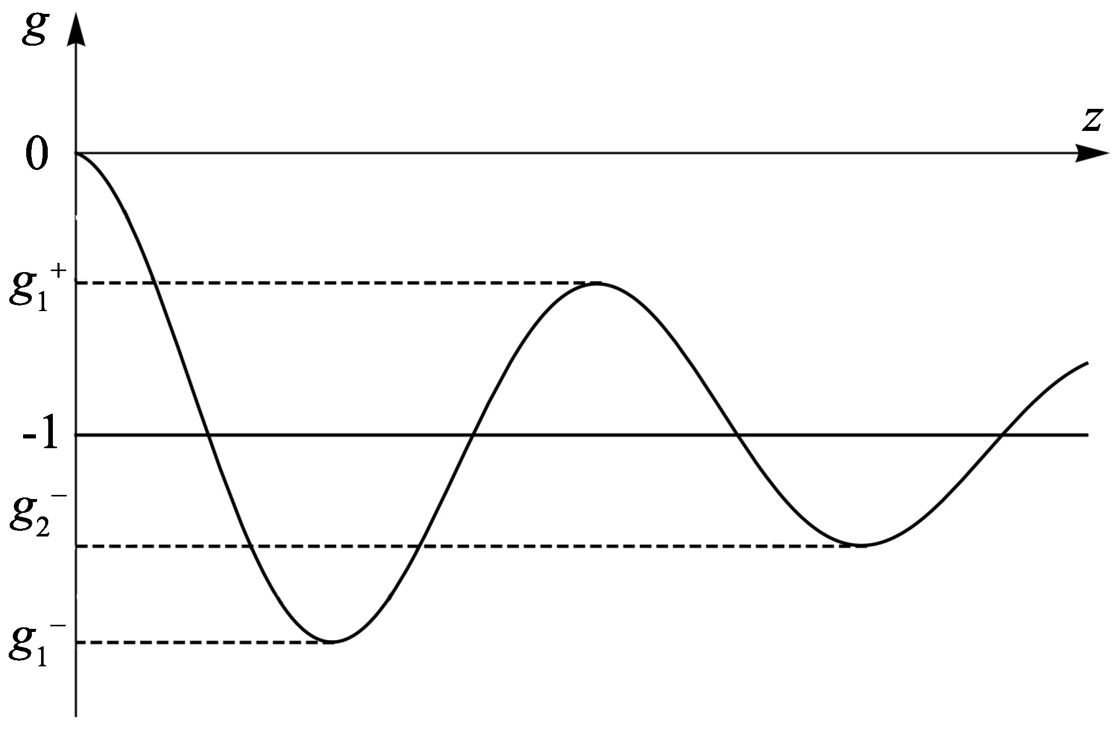
First, let $g_j^{+}$ and $g_j^{-}(j=1,2,\dots )$ be the sequential positive local maxima and minima of the function $g(z)$, respectively (see, Figure 1).

Let, for example, $g_0\in \left(g_1^{+},0\right)$. Then, the value $z_0$ for which $g(z_0)=g_0$ is uniqely determined. If $g_0\in \left(g_1^{-},g_2^{-}\right)$, then there are two such values $z_{10}$ and $z_{20}$ that $g\left(z_{10}\right)=g\left(z_{20}\right)=g_0$, etc. Thus, there is an arbitrary number of values z for which $g(z)=g_0$. But, if $g_0=-1$, then there are infinitely many such values $z_{n0}(n=0,\pm 1,\pm 2,\dots )$, and $z_n=\frac{\pi }{2}(2n+1)$. In what follows, let $a_1$ be a vector determined from the equation $\left(A_0+g_0{D}_0\right)a_1=D_{0}a$. We note that such a vector certainly exists, and $\left(D_0{a}_1,b\right)\ge 0$. We assume that the nonsingularity condition $\left(D_0{a}_1,b\right)>0$ holds.

Let $g_0\in \left(g_1^{+},0\right)$. Then, the root of the equation $g(z)=g_0$ exists and it is unique. Let us now consider the boundary value problem

$$\begin{array}{cc}\hfill \frac{\partial \xi }{\partial \tau }=& {\left(g^{\prime }\left(z_0\right)\right)}^2\left(D_0{a}_1,b\right)\left[\frac{{\partial }^2\xi }{\partial x^2}+2i\Theta \frac{\partial \xi }{\partial x}-{\Theta }^2\xi \right]+\hfill \\ \hfill & +\left(\left(A_1+g_0{D}_1\right)a,b\right)\xi +3g_0{d}_{10}{b}_0\xi {\left|\xi \right|}^2,\hfill \\ \hfill & \xi (\tau ,x+2\pi )\equiv \xi (\tau ,x).\hfill \end{array}$$

(15)

In this case, Theorem 1 also holds in the case when (13) is replaced by (15).

Let $g_0\in \left(g_1^{-},g_2^{-}\right)$. In this case $g\left(z_1\right)=g\left(z_2\right)=g_0$ (see Figure 1). Let the condition

$$3z_1\ne z_2$$

(16)

hold. The system of two boundary value problems

$$\begin{array}{cc}\hfill \frac{\partial {\xi }_j}{\partial \tau }=& {\left(g^{\prime }\left(z_j\right)\right)}^2\left(D_0{a}_1,b\right)\left[\frac{{\partial }^2{\xi }_j}{\partial x^2}+2i{\Theta }_j\frac{\partial {\xi }_j}{\partial x}-{\Theta }_j^2{\xi }_j\right]+\hfill \\ \hfill & +\left(\left(A_1+g_0{D}_1\right)a,b\right){\xi }_j+3g_0{d}_{10}{b}_0{\xi }_j\left[|{\xi }_j{|}^2+2{\left|{\xi }_{j+1}\right|}^2\right],\hfill \\ \hfill & j=1,2\mathrm{and}{\xi }_{j+1}={\xi }_1,\mathrm{if}j=2,{\xi }_j(\tau ,x+2\pi )\equiv {\xi }_j(\tau ,x)\hfill \end{array}$$

plays the role of the boundary value problems (13) and (15). Then, the function

$$\begin{array}{cc}\hfill u(t,x,\epsilon )=& \epsilon a[\sum _{j=1}^2({\xi }_j(\tau ,x)exp\left(i\left(z_j{\epsilon }^{-1}+{\Theta }_j\right)x\right)+\hfill \\ \hfill & +\overline{{\xi }_j}(\tau ,x)exp\left(-i\left(z_j{\epsilon }^{-1}+{\Theta }_j\right)x\right))]+{\epsilon }^{3}U\left(\tau ,x,y_1,y_2\right)\hfill \end{array}$$

satisfies the boundary value problem (3), (4), where $\tau ={\epsilon }^{2}t,y_j=\left(z_j{\epsilon }^{-1}+{\Theta }_j\right)x(j=1,2)$ to within $o\left({\epsilon }^3\right)$.

From this, by analogy, we can obtain systems of the boundary value problems for any $g_0<0$ and $g_0\ne -1$.

The case of $g_0=-1$. Let $z_{n0}=\frac{\pi }{2}(2n+1)$. We assume, for simplicity, that the value of N is a multiple of four: $N=4n$. Then, the values $z_n=z_{n0}{\epsilon }^{-1}$ are integers.

The leading terms of the asymptotic representation are expressed by the formula

$$u(t,x,\epsilon )=\epsilon a\xi (\tau ,x,y)+{\epsilon }^{3}U(\tau ,x,y)\left(\tau ={\epsilon }^{2}t,y=\left(\frac{\pi }{2}{\epsilon }^{-1}\right)x\right).$$

(17)

Here, the dependence on x is $2\pi$-periodic, while the dependence on y is 2-antiperiodic. For $\xi (\tau ,x,y)$ we arrive at the system of the boundary value problems

$$\begin{array}{cc}\hfill \frac{\partial {\xi }_j}{\partial \tau }=& exp\left(-2{\left(\sigma \frac{\pi }{2}(2j+1)\right)}^2\right)\left(D_0{a}_1,b\right)\frac{{\partial }^2{\xi }_j}{\partial x^2}+\hfill \\ \hfill & +\left(\left(A_1+g_0{D}_1\right)a,b\right){\xi }_j+3g_0{d}_{10}{b}_0{F}_j\left({\xi }^3\right),\hfill \end{array}$$

(18)

$$\xi (\tau ,x+2\pi ,y)\equiv \xi (\tau ,x,y),\xi (\tau ,x,y+2)\equiv -\xi (\tau ,x,y).$$

(19)

Let $F_j({\xi }^3)$ be the harmonic $exp\left(i(\frac{\pi }{2}(2j+1)y)\right)$ coefficient of the Fourier series of the function ${\xi }^3$. Formally, the boundary value problem (18) can be written in the compact form in terms of the infinite differentiation operators:

$$\begin{array}{c}\hfill \frac{\partial \xi }{\partial \tau }=K\left(\frac{{\partial }^2}{\partial y^2}\right)(D_0{a}_1,b)\frac{{\partial }^2\xi }{\partial x^2}+\left((A_1-D_1)a,b\right)-3d_{10}{b}_0{\xi }^3,\\ \hfill \xi (\tau ,x+2\pi ,y)\equiv \xi (\tau ,x,y),\xi (\tau ,x,y+2)\equiv -\xi (\tau ,x,y)\end{array}$$

(20)

where $K(p^2)=exp\left(-2{\sigma }^2{p}^2\right)$. If we manage to find the solution of this boundary value problem then, using (17), we can restore the asymptotic solution to the original boundary value problem (3), (4).

3. Bifurcations for Small $\mathit{\sigma }$

In the cases where the coefficients of the couplings become close to the classical diffusion couplings under certain changes in the parameters of the problem, an additional complication of the dynamic properties of the chain occurs. This is due to the fact that, firstly, the bifurcations occur at higher and higher modes, and, secondly, the number of such modes around which the structures are formed grows indefinitely. In these cases, we pass to the dynamics described using the Ginzburg—Landau equation with two spatial variables instead of one spatial variable. The dynamics is obviously more complicated in such cases.

We assume below that the relation

$$\sigma ={\sigma }_1\epsilon$$

(21)

holds for some fixed ${\sigma }_1>0$. In this case, for each z, we have the asymptotic equality

$$g(z)=cosz\left(1-{\sigma }_1^2{\epsilon }^2{z}^2+O({\epsilon }^4)\right)-1.$$

(22)

The number of solutions $z_k$ of the equation $g(z)=g_0$ is unlimited as $\epsilon \to 0$. We now focus on the study of the cases $g_0=-1;g_0=-2;$$g_0\ne -1,-2$, seperately.

3.1. First Case

Let $g_0=-1$. Then, $z_k=\frac{\pi }{2}(2k+1)(k=0,\pm 1,\pm 2,\dots )$ up to $O\left({\epsilon }^2\right)$. First, we assume that $N=4P$ (P is an integer). Then, the expression $z_k{\epsilon }^{-1}$ is also an integer.

We consider the boundary value problem

$$\begin{array}{cc}\hfill \frac{\partial \xi }{\partial \tau }=& \left(D_0{a}_1,b\right)\frac{{\partial }^2\xi }{\partial x^2}+\left(\left(A_1-D_1\right)a,b\right)\xi -3d_{10}{b}_0{\xi }^3,\hfill \\ \hfill & \xi (\tau ,x+2\pi ,y)\equiv \xi (\tau ,x,y)\equiv -\xi (\tau ,x,y+2).\hfill \end{array}$$

(23)

Theorem 2.

Let the condition (21) hold, $g_0=-1$ and N is a multiple of four. Let $\xi (\tau ,x,y)$ be the bounded solution of the boundary value problem (23) for $\tau \to \infty ,x\in [0,2\pi ],y\in [0,4]$. Then, the vector-function

$$u(t,x,\epsilon )=\epsilon a\xi (\tau ,x,y)+{\epsilon }^{3}U(\tau ,x,y),(\tau ={\epsilon }^{2}t,y={\epsilon }^{-1}x)$$

(24)

satisfies the boundary value problem (3), (4) up to $o({\epsilon }^3)$.

Let us then consider the case when the value of N is odd. Let

$${\Theta }_0=\left\{\begin{array}{cc}\frac{3}{4},\hfill & \mathrm{if}N=4P+1,\hfill \\ \frac{1}{4},\hfill & \mathrm{if}N=4P+3.\hfill \end{array}\right.$$

(25)

We consider below the boundary value problem

$$\begin{array}{cc}\hfill \frac{\partial \xi }{\partial \tau }=& \left(D_0{a}_1,b\right)\left[\frac{{\partial }^2}{\partial x^2}+2i\Theta \frac{\partial }{\partial x}-{\Theta }^2\right]\xi +\hfill \\ \hfill & +\left(\left(A_1-D_1\right)a,b\right)\xi -d_{10}{b}_0\left({3\xi \left|\xi \right|}^2+{\overline{\xi }}^{3}exp(-4i{\Theta }_{0}x)\right),\hfill \end{array}$$

(26)

$$\xi (\tau ,x+2\pi ,y)\equiv \xi (\tau ,x,y)\equiv -\xi (\tau ,x,y+2).$$

(27)

Theorem 3.

Let the conditions (21) hold, $g_0=-1$ and N is not a multiple of two. Let $\xi (\tau ,x,y)$ be the bounded solution of the boundary value problem (26), (27) for $\tau \to \infty ,x\in [0,2\pi ],y\in [0,4]$ where ${\Theta }_0$ is defined in (25). Then, the vector-function

$$\begin{array}{cc}\hfill u(t,x,\epsilon )=& \epsilon a[\xi (\tau ,x,y)exp\left(i\left(\frac{\pi }{2}{\epsilon }^{-1}+{\Theta }_0\right)x\right)+\hfill \\ \hfill & +\overline{\xi }(\tau ,x,y)exp\left(-i\left(\frac{\pi }{2}{\epsilon }^{-1}+{\Theta }_0\right)x\right)]+{\epsilon }^{3}U(\tau ,x,y)\hfill \end{array}$$

(28)

satisfies the boundary value problem (3), (4) for $\tau ={\epsilon }^{2}t,y={\epsilon }^{-1}x$ up to $o({\epsilon }^3)$.

It remains to consider the case when

$$N=4P+2$$

and hence ${\Theta }_0=1/2$. We consider the boundary value problem

$$\begin{array}{cc}\hfill \frac{\partial \xi }{\partial \tau }=& \left(D_0{a}_1,b\right)\left[\frac{{\partial }^2}{\partial x^2}+2i{\Theta }_0\frac{\partial }{\partial x}-{\Theta }_0^2\right]\xi +\left(\left(A_1-D_1\right)a,b\right)\xi -\hfill \\ \hfill & -d_{10}{b}_0{\xi }^{3}exp(ix)+{3\xi \left|\xi \right|}^2+3\overline{\xi }{\left|\xi \right|}^{2}exp(-ix)+{\overline{\xi }}^{3}exp(-2ix),\hfill \end{array}$$

(29)

$$\xi (\tau ,x+2\pi ,y)\equiv \xi (\tau ,x,y)\equiv -\xi (\tau ,x,y+2).$$

(30)

Theorem 4.

Let the conditions (21) hold, $g_0=-1$ and $N=4P+2$. Let $\xi (\tau ,x,y)$ be a bounded solution of the boundary value problem (29), (30) for $\tau \to \infty ,x\in [0,2\pi ],y\in [0,4]$ where ${\Theta }_0=1/2$. Then, the vector-function (28) satisfies the boundary value problem (3), (4) as ${\Theta }_0=1/2,\tau ={\epsilon }^{2}t,y={\epsilon }^{-1}x$ up to $o({\epsilon }^{3}t)$.

In order to justify Theorems 2 and 3 under the formulated conditions, it is sufficient to substitute the expressions (23), (28) into (3) and analyze the relations obtained by writing out the coefficients at the first and third powers of $\epsilon$.

Note that the dynamics of the solutions (3), (4) can substantially depent on the parameter ${\Theta }_0$. When ${\Theta }_0=0$, i. e. provided that N is a multiple of four, even the nonlinearity in (23) is different compared to (26) when N is not a multiple of four. Thus, we conclude that a change of only one of the large value N can lead to the significant changes in the (3), (4) dynamics.

3.2. Second Case

Let

$$g_0=-2$$

(31)

and the nonsingularity condition $(D_{0}a,b)\ne 0$ holds. Then, the amplitude $\xi (\tau ,x,y)$ in the asymptotic representation satisfies the boundary value problem

$$\begin{array}{cc}\hfill \frac{\partial \xi }{\partial \tau }=& (D_0,a,b)\left[\frac{1}{2}\left(\frac{{\partial }^2\xi }{\partial x^2}+2i{\Theta }_0\frac{\partial \xi }{\partial x}-{\Theta }_0^2\xi \right)+{\sigma }_1^2\frac{{\partial }^2\xi }{\partial y^2}\right]+\hfill \\ \hfill & +\left((A_1+g_0{D}_1)a,b\right)\xi -2d_{10}{b}_0\Phi (\xi ,x,{\Theta }_0),\hfill \end{array}$$

$$\xi (\tau ,x+2\pi ,y)\equiv \xi (\tau ,x,y)\equiv -\xi (\tau ,x,y+1),$$

$${\Theta }_0=\left\{\begin{array}{cc}0,\hfill & \mathrm{if}N\mathrm{is}\mathrm{even},\hfill \\ \frac{1}{2},\hfill & \mathrm{if}N\mathrm{is}\mathrm{odd},\hfill \end{array}\right.\tau ={\epsilon }^{2}t,y={\epsilon }^{-1}x.$$

$$\Phi \left(\xi ,x,{\Theta }_0\right)=\left\{\begin{array}{c}\left(\xi +\overline{\xi }\right),\mathrm{for}{\Theta }_0=0;\hfill \\ {\xi }^{3}exp(ix)+{3\xi \left|\xi \right|}^2+{\overline{\xi }}^{3}exp(-2ix)+3\overline{\xi }{\left|\xi \right|}^{2}exp(-ix),\mathrm{for}{\Theta }_0=1/2.\hfill \end{array}\right.$$

The function $u(\tau ,x,\epsilon )$ is related with the function $\xi (\tau ,x)$ via the equality

$$u(\tau ,x,\epsilon )=\epsilon a\left(\xi (\tau ,x,y)exp\left(i{\Theta }_{0}x\right)+\overline{\xi }(\tau ,x,y)exp\left(-i{\Theta }_{0}x\right)\right)+{\epsilon }^{3}U(\tau ,x,y).$$

3.3. Third Case

Let

$$g_0\ne -1,g_0\ne -2,g_0=g(h)\mathrm{and}3h\ne 2\pi k,(k=0,\pm 1,\pm 2,\dots )$$

(32)

We present the final boundary value problem for determining the amplitude $\xi (\tau ,x,y)$ in the form of the asymptotic formula

$$\begin{array}{cc}\hfill u(t,x,\epsilon )=& \epsilon a\left(\xi (\tau ,x,y)exp\left(i\left(h{\epsilon }^{-1}+\Theta \right)\right)+\overline{\xi }(\tau ,x,y)exp\left(-i\left(h{\epsilon }^{-1}+\Theta \right)\right)\right)+\hfill \\ \hfill & +{\epsilon }^{3}U(\tau ,x,y),\tau ={\epsilon }^{2}t,y={\epsilon }^{-\frac{1}{2}}x,\hfill \end{array}$$

(33)

$$\begin{array}{cc}\hfill & \frac{\partial \xi }{\partial \tau }=\left(D_0{a}_1,b\right)[{sin}^{2}h·\left(\frac{{\partial }^2\xi }{\partial x^2}+2i\Theta \frac{\partial \xi }{\partial x}-{\Theta }^2\xi \right)+{cos}^{2}h·{\sigma }_1^4\frac{{\partial }^4\xi }{\partial y^4}+\hfill \\ \hfill & +sin2h·{\sigma }_1^2\left(\frac{-i{\partial }^3\xi }{\partial x\partial y^2}+\Theta \frac{{\partial }^2\xi }{\partial y^2}\right)]+\left(\left(A_1+(cosh-1)D_1\right)a,b\right)\xi +3d_{10}{g}_0{b}_0\xi {\left|\xi \right|}^2,\hfill \\ \hfill & \xi (\tau ,x+2\pi ,y)\equiv \xi (\tau ,x,y)\equiv \xi (\tau ,x,y+1).\hfill \end{array}$$

(34)

The analogs of Theorems 2–4 are valid, of course, for the second and third cases. We do not present them here.

4. Conclusions

The chain of the ring coupled Van der Pol systems is considered. It is assumed that the couplings are homogeneous and that the number of elements in the chain is large enough. The transition to a system with a continuous variable is considered. The main attention is drawn to the study of the system with couplings close to diffusion. The critical cases of the Turing type are distinguished in the problem of the stability of the zero equilibrium state. It is shown that all these cases have infinite dimension. The local dynamics of the original systems is investigated. It is found that the considered Turing bifurcations occur on asymptotically high modes or on a whole group of modes with asymptotically large numbers. The special nonlinear equations of parabolic type (equations of the Ginzburg—Landau type) are constructed, which play the role of the first approximation equations for solutions of the original system. It is known (see, for example, [25]) that the dynamics of the Ginzburg—Landau boundary value problems can be quite complex, therefore the same conclusion can be made for the solutions of the considered chain of the Van der Pol systems.

It is worth mentioning one more significant conclusion. The parameter $\Theta$ appears in the constructed parabolic equations. When this parameter is changed, the dynamics can change too [26]. The parameter $\Theta$ ranges infinitely many times from 0 to 1 as $\epsilon \to 0$. Thus, we conclude that the change in the number of elements in the chain (and it is large enough of order ${\epsilon }^{-1}$) even by one leads to the parameter $\Theta$ and hence the dynamics of the original system change significantly.

Note that it is of interest to study chains of nonlinear systems, consisting of a large number of elements, with other type of connections; in particular, with one- and two-way connections, as well as fully connected systems. In addition, it is important to study systems with delayed connections.

References

- Heinrich, G.; Ludwig, M.; Qian, J.; Kubala, B.; Marquardt, F. Collective dynamics in optomechanical arrays. Phys. Rev. Lett. 2011, 107, 043603. [Google Scholar] [CrossRef] [Green Version]
- Zhang, M.; Wiederhecker, G.S.; Manipatruni, S.; Barnard, A.; McEuen, P.; Lipson, M. Synchronization of micromechanical oscillators using light. Phys. Rev. Lett. 2012, 109, 233906. [Google Scholar] [CrossRef] [PubMed] [Green Version]
- Martens, E.A.; Thutupalli, S.; Fourri’ere, A.; Hallatschek, O. Chimera states in mechanical oscillator networks. Proc. Natl. Acad. Sci. USA 2013, 110, 10563–10567. [Google Scholar] [CrossRef] [PubMed] [Green Version]
- Tinsley, M.R.; Nkomo, S.; Showalter, K. Chimera and phase-cluster states in populations of coupled chemical oscillators. Nature Phys. 2012, 8, 662–665. [Google Scholar] [CrossRef] [Green Version]
- Vlasov, V.; Pikovsky, A. Synchronization of a Josephson junction array in terms of global variables. Phys. Rev. E. 2013, 88, 022908. [Google Scholar] [CrossRef] [PubMed] [Green Version]
- Lee, T.E.; Sadeghpour, H.R. Quantum synchronization of quantum van der Pol oscillators with trapped ions. Phys. Rev. Lett. 2013, 111, 234101. [Google Scholar] [CrossRef] [PubMed] [Green Version]
- Kuznetsov, A.P.; Kuznetsov, S.P.; Sataev, I.R.; Turukina, L.V. About Landau — Hopf scenario in a system of coupled self-oscillators. Phys. Lett. A. 2013, 377, 3291–3295. [Google Scholar] [CrossRef] [Green Version]
- Pazó, D.; Matías, M.A. Direct transition to high-dimensional chaos through a global bifurcation. Europhys. Lett. 2005, 72, 176–182. [Google Scholar] [CrossRef]
- Osipov, G.V.; Pikovsky, A.S.; Rosenblum, M.G.; Kurths, J. Phase synchronization effects in a lattice of nonidentical Rossler oscillators. Phys. Rev. E 1997, 55 Pt A, 2353–2361. [Google Scholar] [CrossRef] [Green Version]
- Thompson, J.M.T.; Stewart, H.B. Nonlinear Dynamics and Chaos; Wiley: Chichester, UK, 1986. [Google Scholar]
- Simonotto, E.; Riani, M.; Seife, C.; Roberts, M.; Twitty, J.; Moss, F. Visual Perception of Stochastic Resonance. Phys. Rev. Lett. 1997, 78, 1186. [Google Scholar] [CrossRef]
- Kuramoto, Y. Chemical Oscillations, Waves and Turbulence; Springer: Berlin, Germany, 1984; 164p. [Google Scholar]
- Afraimovich, V.S.; Nekorkin, V.I.; Osipov, G.V.; Shalfeev, V.D. Stability, Structures and Chaos in Nonlinear Synchronization Networks; World Scientific: Singapore, 1994. [Google Scholar]
- Pikovsky, A.S.; Rosenblum, M.G.; Kurths, J. Synchronization: A Universal Concept in Nonlinear Sciences; Cambridge University Press: Cambridge, UK, 2001. [Google Scholar]
- Osipov, G.V.; Kurths, J.; Zhou, C. Synchronization in Oscillatory Networks; Springer: Berlin, Germany, 2007. [Google Scholar]
- Turing, A.M. The chemical basis of morphogenesis. Philos. Trans. R. Soc. Lond. B. Biol. Sci. 1952, 237, 37–72. [Google Scholar]
- Castets, V.; Dulos, E.; Boissonade, J.; Kepper, P.D. Experimental evidence of a sustained standing Turing-typenonequilibrium chemical pattern. Phys. Rev. Lett. 1990, 64, 2953–2956. [Google Scholar] [CrossRef] [PubMed] [Green Version]
- Fields, R.J.; Burger, M. Oscillations and Travelling Waves in Chemical Systems; Wiley: New York, NY, USA, 1985; 681p. [Google Scholar]
- Vanag, V.K.; Epstein, I.R. Packet waves in a reaction-diffusion system. Phys. Rev. Lett. 2002, 88, 088303. [Google Scholar] [CrossRef] [PubMed] [Green Version]
- Yang, L.; Berenstein, I.; Berenstein, I.R. Segmented waves from a spatiotemporal transverse wave instability. Phys. Rev. Lett. 2005, 95, 038303. [Google Scholar] [CrossRef] [PubMed] [Green Version]
- Kashchenko, I.S.; Kashchenko, S.A. Dynamics of the Kuramoto equation with spatially distributed control. Comm. Nonlin. Sci. Numer. Simulat. 2016, 34, 123–129. [Google Scholar] [CrossRef]
- Kashchenko, S.A. On quasinormal forms for parabolic equations with small diffusion. Sov. Math. Dokl. 1988, 37, 510–513. Available online: http://www.ams.org/mathscinet-getitem?mr=0947229 (accessed on 5 September 2022).
- Kaschenko, S.A. Normalization in the systems with small diffusion. Int. J. Bifurc. Chaos Appl. Sci. Eng. 1996, 6, 1093–1109. [Google Scholar] [CrossRef]
- Kashchenko, S.A. Dynamics of advectively coupled Van der Pol equations chain. Chaos: Interdiscip. J. Nonlinear Sci. 2021, 31, 033147. [Google Scholar] [CrossRef]
- Akhromeeva, T.S.; Kurdyumov, S.P.; Malinetskii, G.G.; Samarskii, A.A. Nonstationary Structures and Diffusion Chaos; Nauka: Moscow, Russia, 1992; 544p. [Google Scholar]
- Kashchenko, I.S.; Kashchenko, S.A. Infinite Process of Forward and Backward Bifurcations in the Logistic Equation with Two Delays. Nonlinear Phenom. Complex Syst. 2019, 22, 407–412. [Google Scholar] [CrossRef]
Figure 1.
Plot .
Publisher’s Note: MDPI stays neutral with regard to jurisdictional claims in published maps and institutional affiliations. |
© 2022 by the author. Licensee MDPI, Basel, Switzerland. This article is an open access article distributed under the terms and conditions of the Creative Commons Attribution (CC BY) license (https://creativecommons.org/licenses/by/4.0/).
Share and Cite
MDPI and ACS Style
Kashchenko, S. Infinite Turing Bifurcations in Chains of Van der Pol Systems. Mathematics 2022, 10, 3769. https://doi.org/10.3390/math10203769
AMA Style
Kashchenko S. Infinite Turing Bifurcations in Chains of Van der Pol Systems. Mathematics. 2022; 10(20):3769. https://doi.org/10.3390/math10203769
Chicago/Turabian StyleKashchenko, Sergey. 2022. "Infinite Turing Bifurcations in Chains of Van der Pol Systems" Mathematics 10, no. 20: 3769. https://doi.org/10.3390/math10203769
Note that from the first issue of 2016, this journal uses article numbers instead of page numbers. See further details here.