Interference of Non-Hermiticity with Hermiticity at Exceptional Points

Abstract

The recent growth in popularity of the non-Hermitian quantum Hamiltonians $H\left(\lambda \right)$ with real spectra is strongly motivated by the phenomenologically innovative possibility of an access to the non-Hermitian degeneracies called exceptional points (EPs). What is actually presented in the present paper is a perturbation-theory-based demonstration of a fine-tuned nature of this access. This result is complemented by a toy-model-based analysis of the related details of quantum dynamics in the almost degenerate regime with $\lambda \approx {\lambda }^{\left(EP\right)}$. In similar studies, naturally, one of the decisive obstacles is the highly nontrivial form of the underlying mathematics. Here, many of these obstacles are circumvented via several drastic simplifications of our toy models—i.a., our N by N matrices $H\left(\lambda \right)=H^{\left(N\right)}\left(\lambda \right)$ are assumed real, tridiagonal and $\mathcal{PT}$-symmetric, and our $H^{\left(N\right)}\left(\lambda \right)$ is assumed to be split into its Hermitian and non-Hermitian components staying in interaction. This is shown to lead to several remarkable spectral features of the model. Up to $N=8$, their description is even shown tractable non-numerically. In particular, it is shown that under generic perturbation, the “unfolding” removal of the spontaneous breakdown of $\mathcal{PT}$-symmetry proceeds via intervals of $\lambda$ with complex energy spectra.

1. Introduction

In the conventional quantum mechanics of textbooks [1], the unitarity of evolution is interpreted as a consequence of the self-adjointness of the Hamiltonian in the Schrödinger picture [2]. Naturally, the same connection applies also in the Heisenberg picture and in any other formulation of standard quantum mechanics. In the Schrödinger picture, a “quasi-Hermitian operator” [3] modification of this approach was offered, in 1992, by Scholtz et al. [4]. These authors characterized the conventional mathematical interpretation of the unitarity of the evolution as “somewhat restrictive.” Assuming that in a suitable pre-selected “mathematical” Hilbert space ${\mathcal{H}}_{math}$, a bound-state Hamiltonian H appears non-Hermitian, it has been argued that the system in question can still acquire “the normal quantum mechanical interpretation” in another, “physical” Hilbert space ${\mathcal{H}}_{phys}$ endowed with an amended, Hamiltonian–Hermitizing inner-product metric $\Theta =\Theta \left(H\right)\ne I$.

The idea of the Hermitization of the operators of observables via an ad hoc amendment of the inner product in ${\mathcal{H}}_{phys}$ is currently widely used by physicists (see, e.g., the recent reviews [5,6,7]). At the same time, deeper analyses by mathematicians (see, e.g., [8,9,10]) reveal that the formalism (to be called here quasi-Hermitian quantum mechanics, QHQM) still requires a more rigorous critical re-evaluation of the conditions and boundaries of its applicability.

The doubts and critical voices—which in fact motivated also our present study—appeared also among physicists. In 2007, in particular, Hugh Jones studied the problem of scattering [11,12], and he noticed that in certain quantum systems characterized by the coexistence, mixture and interaction between a non-Hermitian and a Hermitian Hamiltonian, the QHQM theory of scattering may really become conceptually inconsistent. Incidentally, what followed in the research was “the weakening of emphasis on the explicit constructions of metrics” [9]. The crisis emerged, but “it did not hit the models using effective Hamiltonians,” for which “their phenomenological interpretation does not require any construction of the metric” [9].

Mathematical consistency of the QHQM theory of unitary systems can still be achieved after its more consequent formulation [4,6,9]. The price to pay is that the choice (or rather the construction) of the internally consistent pairs of a Hamiltonian H (which is admitted non-Hermitian in ${\mathcal{H}}_{math}$) and of the ad hoc Hermitizing inner-product metric $\Theta \left(H\right)$ (which must be Hermitian in ${\mathcal{H}}_{math}$) is technically difficult, especially, as emphasized by Jones [12], in the scattering dynamical regime. Indeed, one of Jones’ main conclusions was that in the innovative QHQM framework it becomes difficult to avoid certain fairly deep conceptual paradoxes (for a more detailed explanation, see Section 2 below).

In the literature, an escape out of the dilemma has been found in an ad hoc restriction of the admissible non-Hermitian Hamiltonians, say, to their bounded-operator subclass [4] or to their strictly confining bound-states-generating forms [13]. Along these lines, it has been found that the technical aspects of the conceptual analysis of the non-Hermitian models appear perceptibly less complicated in the narrower unitary bound-state dynamical context than in the full-fledged quantum theory, including scattering (see, nevertheless, a fully consistent QHQM model of scattering in [14]).

Alternatively, attention can be also turned to the study of the open, non-unitary quantum systems with resonances [15]. This theory uses a more traditional terminology which dates back to Feshbach’s enormously productive introduction of the concept of the energy-dependent and manifestly non-Hermitian “effective” Hamiltonians, $H_{\left(eff\right)}\ne H_{\left(eff\right)}^{†}$, defined as projected and acting in the so called model subspace of the full Hilbert space [16]. Needless to say, in such a very general, essentially non-unitary framework, there emerges no possibility (and also no need) for a search for a Hermitian partner of $H_{\left(eff\right)}$.

In both the unitary and non-unitary contexts, several serendipitious phenomenological benefits have been found during the discussions on the role of the so-called Kato exceptional points (EP, [17]). In this respect, for the time being, let us only remind the readers that even after the restriction of attention to the Hermitizable Hamiltonians with the discrete and real spectra, it has been found that the QHQM simulation of the dynamics using the nontrivial metrics $\Theta$ becomes much more flexible than its traditional Hermitian forms in which the metric remains fixed and trivial, $\Theta =I$.

The existence of the new model-building freedom using the non-Hermiticity opens new horizons not only via the inventions of the pragmatically oriented phenomenological models (say, of quantum phase transitions [18,19,20,21,22,23,24,25]), but also via some more formal mathematical toy-model constructions (cf., e.g., [26,27,28]). In both the open and closed quantum systems, one even encounters and identifies various genuine quantum analogues of what is called, in non-quantum physics, evolution bifurcations, or in the Thom-inspired terminology, “catastrophes” [29,30]. In all of these contexts, the key role is played, indeed, by the above-mentioned concept of the Kato’s exceptional points. In what follows, this subject is to be developed further.

For methodical purposes, the form of our argumentation and toy models will be chosen to be as simple as possible. In fact, our study of interaction between the comparatively well separated Hermitian and non-Hermitian components of the Hamiltonian will be essentially simplified by not involving the systems with scattering, and by the technically motivated restriction of our analysis to certain EP-related phenomena supported by the N by N matrix forms of $H=H^{\left(N\right)}$ with even $N=2J$. One of the key merits of our results and conclusions will be that they will be mostly algebraic and non-numerical, even when the matrix size N itself will be admitted to be arbitrarily large.

2. Non-Hermitian and Hermitian Operators in Interaction

The key appeal of the use of the quantum non-Hermitian Hamiltonians is that they admit access to Kato’s exceptional-point (EP, [17]) dynamical singularities. In particular, in some special unitary QHQM systems living in the vicinity of these singularities, the non-Hermiticity might help to mimic, e.g., the quantum phase transitions [18,25]. Still, on both the mathematical and phenomenological sides, the subject is full of open questions. In this framework, we intend to address, first of all, those aspects of the generic Hermitian–non-Hermitian interference theory which are related to the Jones ansatz

$$H=H_1+H_2+H_{coupling},H_1=H_1^{†},H_2\ne H_2^{†}.$$

(1)

We developed a class of models elucidating some of the general phenomenological and mathematical consequences of this ansatz. In addition to the mathematical orientation of our present study, we also stress the existence of a parallel motivation for our project: the study of the interactions (1) and of the EPs in physics.

2.1. Motivation: The Access to EPs in Quantum Physics

For any parameter-dependent family of non-Hermitian quantum Hamiltonians $H=H\left(\lambda \right)$ in (1), one can expect the existence of a “critical value” of the parameter at which the spectrum ceases to be real [13]. In the language of mathematics, such a “critical value” of the coupling is to be identified with Kato’s EP parameter ${\lambda }^{\left(EP\right)}$. Recently, the concept acquired an immediate experimental meaning in several phenomenological applications ranging from relativistic quantum mechanics [31,32] and quantum cosmology [33,34] to the efficient toy-model simulations of the various forms of quantum-phase transitions [35].

Many years ago, the use of the EPs caused a change in the paradigm in the mathematical foundations of the perturbation theory of linear operators [17,36]. Still, until recently, the concept did not seem to have found immediate applications in conventional, textbook quantum physics [1]. Indeed, in the context of the theoretical quantum physics of unitary systems, the typical EP singularities were complex that their experimental visibility remained, necessarily, indirect.

In his old but still fully authoritative monograph [17], Kato emphasized that for a given self-adjoint Hamiltonian $\mathfrak{h}\left(\lambda \right)={\mathfrak{h}}^{†}\left(\lambda \right)$ which is analytic in the parameter, our knowledge of the (complex) quantities ${\lambda }^{\left(EP\right)}$ opens the way towards a rigorous determination of the radius of convergence R of the most common Rayleigh–Schrödinger perturbation series for the bound state energies $E_n\left(\lambda \right)$. This leads to a paradox that in one of the most prominent examples of the applicability of the Rayleigh–Schrödinger perturbation series to the quartic anharmonic quantum oscillator ${\mathfrak{h}}^{\left(AHO\right)}\left(\lambda \right)=p^2+\lambda q^4$, the authors of [37] (who managed to localize practically all of the not too large values of ${\lambda }_{(m,n)}^{(EP/AHO)}$ (numbered by the two non-negative integers) numerically) came to the disappointing conclusion that $R^{\left(AHO\right)}=0$.

In the language of experimental physics, an analogous discouraging conclusion is that every EP value ${\lambda }^{\left(EP\right)}$ of any variable parameter entering any operator representing an observable quantity must necessarily remain unphysical because $\mathrm{Im}{\lambda }^{\left(EP\right)}\ne 0$. Thus, in experiments, even the EP singularity (with a sufficiently small size of its imaginary part $\mathrm{Im}{\lambda }^{\left(EP\right)}$) only manifests its presence via the well known phenomenon of the so called avoided level crossing.

During the recent developments of the study of EPs, fortunately, several “dark clouds” (e.g., the above-mentioned and rather unpleasant rigorous proof of the manifest divergence of the AHO series) appeared to also have a silver lining (in the context of perturbation theory, for example, several alternative, sophisticated, but unexpectedly efficient resummation methods have been discovered as a consequence [36]). The subsequent turn in attention to the analytic continuation methods resulted, finally, in the fairly unexpected discovery of Bender and Boettcher [38] that in some quantum models characterized by an analytically continued and manifestly non-Hermitian Hamiltonian $H\left(\lambda \right)\ne H^{†}\left(\lambda \right)$, the bound state energies $E_n\left(\lambda \right)$ (and at least some of the related EP values ${\lambda }_{(m,n)}^{\left(EP\right)}$ of the parameter) still might keep their traditional experimental bound-state meanings, while being real, discrete and bounded from below. On these grounds, Bender with Boettcher [38] conjectured that there might exist certain manifestly non-Hermitian realizations of quantum systems which could still admit the conventional probabilistic interpretation and properties. Their claim has been illustrated by the manifestly non-Hermitian ordinary differential Hamiltonians

$$H^{\left(BB\right)}\left(\lambda \right)=-\frac{d^2}{d{x}^2}+g(\lambda ,x)x^2,g(\lambda ,x)={\left(\mathrm{i}x\right)}^{\lambda },x\in (-\infty ,\infty ).$$

(2)

which “may be viewed as analytic continuations of conventional theories” [38]. In the limit $\lambda \to 0$, indeed, their toy model $H^{\left(BB\right)}\left(\lambda \right)$ coincides with the standard self-adjoint harmonic oscillator with equidistant spectrum $E_n^{\left(BB\right)}\left(0\right)=2n+1$.

Equation (2) represents one of the most popular examples of an operator which is manifestly non-Hermitian (in $L^2\left(\mathbb{R}\right)$) but still has a spectrum which is real, discrete and bounded from below [38]. Thus, it has long been believed that such an operator might represent a more or less standard quantum bound-state Hamiltonian “which allows for the normal quantum-mechanical interpretation” [4]. Unfortunately, a deeper analysis of the operator revealed that these expectations cannot be fulfilled [39]. In a partial analogy with the above-mentioned $R^{\left(AHO\right)}=0$ paradox, the limiting transition $H^{\left(BB\right)}\left(\lambda \right)\to H^{\left(BB\right)}\left(0\right)$ has to be interpreted as discontinuous. Indeed, even the smallest decrease in the exponent $\lambda$ below zero leads to an abrupt loss of the reality of the whole high-energy part of the spectrum. Only a few low-lying levels $E_n^{\left(BB\right)}\left(\lambda \right)$ with $n=0,1,\dots ,n_{max}\left(\lambda \right)$ remain real; the upper bound integer $n_{max}\left(\lambda \right)$ grows as a function of $\lambda \in (-2,2)$, between its minimum $n_{max}\left({\lambda }_{min}\right)=0$ at ${\lambda }_{min}\in (-2,-0.57793)$ and its maximum $n_{max}\left({\lambda }_{max}\right)=\infty$, say, in the interval of ${\lambda }_{max}\in [0,2)$.

With ${\lambda }_{max}\in [0,2)$, people still felt inclined to treat the evolution generated by Hamiltonian (2) as one of the most impressive (i.e., local-interaction-controlled) benchmark examples of the quantum evolution which is “hiddenly” unitary. In brief, the widely accepted belief was that the hidden unitarity alias quasi-unitarity of the model is equivalent to the conventional unitarity [4,6]). In connection with the local-interaction-controlled family of models (2), unfortunately, the latter optimistic expectations remained unfulfilled: In 2012, Siegl with Krejčiřík considered their special case with $\lambda =1$ [39], and they proved, using the rigorous methods of functional analysis, that, “There is no quantum-mechanical Hamiltonian associated with it” (i.e., with the cubic-interaction BB operator $H^{\left(BB\right)}\left(\lambda \right)$ at $\lambda =1$) [39]. Moreover, these authors also added that, “The method …of the disproval …does not restrict the particular Hamiltonian (2). It also applies …to many others.” [39].

In such a situation, obviously, it was necessary to turn attention to the other sufficiently elementary toy models.

2.2. Paradox of Non-Locality of Complex Delta-Function Interactions

In our present paper, the following words of warning are important. Firstly, we accept the fact that Siegl’s and Krejčiřík’s disproof of the quasi-Hermiticity of Bender’s and Boettcher’s (or, more precisely, Caliceti’s [40] and Bessis’ [41] or Alvarez’s [42]) imaginary cubic benchmark example is correct. After all, their observations appeared to be reconfirmed in a few other studies [10,26,27]. Secondly, we are persuaded that the criticism of the specific model(s) does not imply a disproval of the applicability and appeal of the abstract quantum mechanics in its innovative quasi-Hermitian formulation, as provided, say, by reviews [4,6,43]. Hence, we believe that the alternative, still sufficiently transparent benchmark models have to be sought. Last but not least, we oppose the methodical skepticism connected with the formalism and formulated recently in several independent studies [44]. Thus, in our present paper we express and constructively support our belief that the quasi-Hermitian quantum theories, “originally proposed with the aim of extending standard quantum theory by relaxing the Hermiticity constraint on Hamiltonians” [44], really did reach the goal.

In the dynamical scenarios characterized by the interference between Hermitian and non-Hermitian components in the Hamiltonian (1), the theoretician may encounter “a quandary” [11]. The picture of physics may easily become deeply unsatisfactory in both of the alternative representation Hilbert spaces, ${\mathcal{H}}_{math}$ and ${\mathcal{H}}_{phys}$. A more detailed description of the dilemma has been offered by Jones [45]. In his paper, the author studied hypothetical scattering controlled by the delta-function interactions in Hamiltonian $H=H_1\left(\alpha \right)+H_2(\beta ,L)$ where

$$H_1\left(\alpha \right)=-\frac{{\hslash }^2}{2m}\frac{d^2}{d{x}^2}-\alpha \delta \left(x\right)=H_1^{†}\left(\alpha \right)$$

(3)

and

$$H_2(\beta ,L)=-\frac{{\hslash }^2}{2m}\frac{d^2}{d{x}^2}+\mathrm{i}\beta \left[\delta (x-L)\delta (x+L)\right]\ne H_2^{†}(\beta ,L).$$

(4)

In the conventional Hilbert space ${\mathcal{H}}_{math}$, the first component of the Hamiltonian was Hermitian, but its second part has been chosen as non-Hermitian, i.e., all of the three independent parameters, $\alpha$, $\beta$, and L were chosen to be real. After a detailed analysis based on perturbation theory, the Jones’ conclusion was that “the conceptual issues arise” [12,45].

In reference [45], in particular, we read that for the scattering states “one can …no longer talk in terms of reflection and transmission coefficients,” and that “the only satisfactory resolution of this dilemma is to treat the non-Hermitian scattering potential as an effective one, …accepting that this …may well involve the loss of unitarity” [45].

The puzzle found its resolution in [46]. It has been revealed there that in the slightly counterintuitive QHQM framework, a very careful experimental and theoretical definition of the scattering setup is obligatory. More specifically, the source of the apparent inconsistencies has been found to lie in an inappropriate nature of the non-Hermitian scatterer $H_2$ of Equation (4) because its spatial range appeared infinite in the physical Hilbert space ${\mathcal{H}}_{phys}$. Thus, paradoxically but understandably, the phenomenologically natural physical finite-range requirement excludes the delta-function model of Equation (4) as unacceptable.

3. Finite-Dimensional Toy-Model Hamiltonians

The ill-conditioned nature of the numerical search for the EPs in general cases [47] was one of the reasons why we choose, in our present toy model Hamiltonians (10), the equidistant main diagonal. Indeed, in the light of our older paper [48], such a choice can be perceived as technically important, leading to an enormous simplification of the process of the localization of its EP-related extreme-physics limits. Needless to add that by the needs of phenomenology, such a localization is very well motivated because in the models of some fairly realistic quantum systems, the values of the EPs become related to the instants of a genuine quantum phase transition [25].

3.1. Partitioned Structure of the Relevant Hamiltonians

In the realistic models connecting Hermitian and non-Hermitian components in an operator of an observable quantity, the study of the mutual interference of the components is difficult. The mathematical methods of the corresponding physics-oriented analysis of the system’s properties are usually approximate. For illustration, we may recall Bender’s and Jones’ paper [13], in which they considered several “realistic,” differential-operator models which really appeared tractable by the conventional perturbation theory in its leading-order form.

In loc. cit., the authors also admitted that the insight into the features of the scattering models is less easy. At the same time, they reconfirmed the conceptual consistency of the QHQM approach to the class of the mixed, “composite,” three-component, bound-state Hamiltonians (1) “by means of a number of soluble models” [13]. These authors have shown that in all of their models, “the energy remains real for small values of the coupling constant” in $H_{coupling}$ [13]. On the methodical level, these conclusions were further supported by the four-by-four complex-matrix sample of superposition (1).

The latter argument did not sound too persuasive. Its authors treated even their elementary small-matrix model by the mere brute-force numerical diagonalization. Indirectly, the approximate nature of the result contributed to the motivation of our present paper. We intend to complement the analysis of the Hermiticity–non-Hermiticity interference and interfaces by its extension to a family of the bound-state models which would be solvable exactly. We will restrict our attention to the specific real-matrix Hamiltonians characterized by an arbitrary finite (and for the sake of definiteness, even) matrix dimension $N=2M+2K$. In this manner, we complement the above-mentioned studies based on the mere approximate estimates.

More specifically, our present toy model Hamiltonians all have the block-tridiagonal partitioned-matrix structure:

$$H=H^{\left(N\right)}=\left[\begin{array}{ccc}A& U_{+}& 0\\ U_{-}& C& V_{+}\\ 0& V_{-}& B\end{array}\right].$$

(5)

In the notation of Equation (1), the two M by M submatrices $A=A^{†}$ and $B=B^{†}$ will then define the block-diagonal Hermitian sub-Hamiltonian component of the full Hamiltonian:

$$H_1=\left[\begin{array}{ccc}A& 0& 0\\ 0& 0& 0\\ 0& 0& B\end{array}\right]=H_1^{†}.$$

The complementary non-Hermitian component $H_2\ne H_2^{†}$ of Equation (1) will only contain the single non-vanishing $2K$ by $2K$ submatrix $C\ne C^{†}$. The remaining four non-vanishing submatrices, $U_{\pm }$ and $V_{\pm }$, will finally determine the interaction Hamiltonian $H_{coupling}$ forming a suitably variable coupling between the latter two sub-Hamiltonians, and are able to cause various forms of the interference between the non-Hermiticity and Hermiticity of the two respective subsystems.

3.2. $\mathcal{PT}$-Symmetry Requirement and Reparametrization

The main goal of our construction of the benchmark models (5) was twofold. Firstly, we searched for the models in which the integers M and K (specifying the submatrix dimensions) can be arbitrary. A wealth of the phenomenologically interesting spectral structures may be then expected to occur. Secondly, we succeed in keeping our study non-numerical. We obtain and describe a family of benchmark Hamiltonians for which the demonstration of the reality of the spectrum and/or of its loss will be algebraic and rigorous.

We will see that the unitary, closed-system evolution regime characterized by the reality of spectrum need not necessarily require the smallness of the couplings. In the mathematically not-less-interesting complex-spectrum scenarios, the evolution proceeds in the open-system regime. One changes the philosophy, and in the words of reference [45], “accepts that unitarity is not conserved, essentially because we are dealing with a subsystem of a larger system whose physics has not been taken fully into account.”

In the methodical framework, our present choice of a specific realization of the family of Hamiltonians (5) will be restricted by the following three requirements.

• [A] T elements of H lying on the main diagonal will form a real and equidistant sequence simulating the spectrum of the most common harmonic oscillator;
• [B] As long as a broad class of general matrices can be routinely tridiagonalized, we assume that all of our Hs are tridiagonal. Moreover, for the methodical reasons formulated in [49], their off-diagonal part was chosen to be antisymmetric;
• [C] After a finite-dimensional truncation, our benchmark N by N matrices $H=H^{\left(N\right)}$ is required to be $\mathcal{PT}$-symmetric, $H\mathcal{PT}=\mathcal{PT}H$ [50,51]. Here, $\mathcal{P}$ is defined as the antidiagonal unit matrix (“parity” [49]), and the symbol $\mathcal{T}$ represents the antilinear Hermitian conjugation mimicking the time reversal [38].

In the light of the first two requirements, [A] and [B], we may start our considerations from the anharmonic-oscillator-like, infinite-dimensional tridiagonal matrix

$$H^{(\infty )}=\left[\begin{array}{ccccc}1& a_1& 0& 0& \dots \\ -a_1& 3& a_2& 0& \dots \\ 0& -a_2& 5& a_3& \ddots \\ 0& 0& -a_3& 7& \ddots \\ ⋮& ⋮& \ddots & \ddots & \ddots \end{array}\right].$$

(6)

Such an infinite-dimensional matrix Hamiltonian is composed of the main diagonal (which represents the equidistant energy spectrum of an unperturbed harmonic oscillator) and of the off-diagonal “perturbation” having the maximally elementary form of a real and antisymmetric two-diagonal multi-parametric anharmonic interaction $H^{(\infty )}=H^{\left(HO\right)}+V(a_1,a_2,\dots )$.

In a way well motivated, say, in the context of the numerical and/or variational calculations, one usually truncates the infinite-dimensional matrix (6) to its finite-dimensional N by N matrix alternatives. Then, we may trivially replace $H_{nn}\to H_{nn}-constant$ (i.e., shift the conventional origin of the energy scale). We may also impose the $\mathcal{PT}$-symmetry requirement [C]. All this led to our ultimate replacement of Equation (6) by the matrix

$$H^{\left(2J\right)}=\left[\begin{array}{cccccccc}1-2J& a_1& 0& 0& \dots & \dots & 0& 0\\ -a_1& 3-2J& a_2& 0& 0& \dots & \dots & 0\\ 0& -a_2& \ddots & \ddots & \ddots & \ddots & & ⋮\\ 0& \ddots & \ddots & -1& a_J& 0& \ddots & ⋮\\ ⋮& \ddots & 0& -a_J& 1& \ddots & \ddots & 0\\ ⋮& & \ddots & \ddots & \ddots & \ddots & a_2& 0\\ 0& \dots & \dots & 0& 0& -a_2& 2J-3& a_1\\ 0& 0& \dots & \dots & 0& 0& -a_1& 2J-1\end{array}\right].$$

(7)

We have to distinguish between the parameters $a_j$ which are real (for them, the measure of non-Hermiticity $(-a_j)-\left(a_j^{☆}\right)$ is maximal) and which are purely imaginary (for them, the Hermiticity is guaranteed since $(-a_j)-\left(a_j^{☆}\right)=0$). For this reason it makes sense to reparametrize

$$a_j=\sqrt{z_j},j=1,2,\dots ,J.$$

(8)

In what follows, we will simplify the situation by an additional ordering assumption

$$z_1<z_2<\dots <z_J.$$

(9)

This will reduce the menu of the eligible partitionings of our Hamiltonians $H^{\left(N\right)}$ to the mere triply partitioned pattern of Equation (5). In this equation, due to the assumption of the $\mathcal{PT}$-symmetry of $H^{\left(N\right)}$, one merely has to consider the interaction between the two Hermitian M by M submatrices A and B and the single non-Hermitian $2K$ by $2K$ submatrix C. At a fixed $N=2J=2M+2K$, naturally, we only have a single variable dimension (i.e., M or K) at our disposal, the value of which depends on the parameters $z_j$ in a way classified in

Table 1. Dimensions in partitioning (5) under assumption (9).

	${\mathit{z}}_1>0$	${\mathit{z}}_1\le 0$	${\mathit{z}}_2\le 0$	…	${\mathit{z}}_{\mathit{J}-1}\le 0$	−
	−	${\mathbf{z}}_{\mathbf{2}}>\mathbf{0}$	${\mathbf{z}}_{\mathbf{3}}>\mathbf{0}$	…	${\mathbf{z}}_{\mathbf{J}}>\mathbf{0}$	${\mathbf{z}}_{\mathbf{J}}=\mathbf{0}$
M	−	1	2	…	$J-1$	J
K	J	$J-1$	$J-2$	…	1	−

.

4. Exceptional Points

In the mathematically-oriented context of our present paper, let us point out that given a single-parameter-dependent tridiagonal matrix $H=H\left(\lambda \right)$, the search for its EP singularities ${\lambda }^{\left(EP\right)}$ is difficult, even if we keep the main diagonal equidistant and parameter-independent. For an illustration of the specific mathematical difficulties emerging in the non-equidistant diagonal-element cases, we recommend the details of the EP construction, as described in [47]. It has been shown there that the straightforward, brute-force localization of the values of $\lambda ={\lambda }^{\left(EP\right)}$ is truly an extremely ill-conditioned numerical task in general.

From the perspective of physics, it is also useful to keep in mind that the eigenstates of the limit $H\left({\lambda }^{\left(EP\right)}\right)$ do not form a basis [17]. From the QHQM point of view, this means that the system in question only remains observable near but not at the manifestly unphysical EP limit, hence the boundary of the domain of the admissible physical couplings or other parameters [6]. For all of these reasons, from time to time, we will simplify our argumentation by a return from the fully general dimension $N=2J$ to its various comprehensive exemplifications.

4.1. Illustrative $N=8$ Example

Without the assumption of the $\mathcal{PT}$-symmetry of $H\left(\lambda \right)$, even the equidistance of the elements on the main diagonal would not be enough, leaving the printed version of the secular polynomial $P\left(E\right)=det(H-EI)$ (evaluated via the computer-assisted symbolic manipulations in MAPLE [52]) still prohibitively long. Fortunately, after the change of variables (8), we managed to shorten the printout of $P\left(E\right)$ to an acceptable length.

The mere four rows were needed at the not-too-small $N=8$. For this reason, such a choice is also suitable for our present methodical purposes, since the structure of our Hamiltonians (7) is well sampled by the model with $J=4$:

$$H^{\left(8\right)}=H^{\left(8\right)}(a_1,\dots ,a_4)=\left[\begin{array}{cccccccc}-7& a_1& 0& 0& 0& 0& 0& 0\\ -a_1& -5& a_2& 0& 0& 0& 0& 0\\ 0& -a_2& -3& a_3& 0& 0& 0& 0\\ 0& 0& -a_3& -1& a_4& 0& 0& 0\\ 0& 0& 0& -a_4& 1& a_3& 0& 0\\ 0& 0& 0& 0& -a_3& 3& a_2& 0\\ 0& 0& 0& 0& 0& -a_2& 5& a_1\\ 0& 0& 0& 0& 0& 0& -a_1& 7\end{array}\right].$$

(10)

As long as every submatrix of $H_{coupling}$ (i.e., $U_{\pm }$ and $V_{\pm }$ in (5)) will have, by construction, a single non-vanishing matrix element, the above-introduced change of variables $a_j\to z_j$ enables us to switch, easily, between the Hermitian and non-Hermitian forms of the coupling matrix itself. At a fixed $N=8$, it makes sense to avoid the need for subscripts and write

$$a_1:=\sqrt{D};a_2:=\sqrt{C};a_3:=\sqrt{B};a_4:=\sqrt{A}.$$

(11)

The use of a fixed N will shorten the necessary compact review of some older relevant results in the literature. Among the most relevant ones, let us mention the descriptions of the less standard QHQM formalism. Although its short summary may be found in Appendix A below, it is necessary to remind the readers that one of the key practical benefits offered by such a formalism lies in the possibility of the description of the various (i.e., both closed and open) quantum systems in an arbitrarily small vicinity of their exceptional-point (EP, [17]) degenerate extremes.

This has both its mathematical and physical aspects, both of which may be well illustrated by the specific choice of $N=8$. Using reparametrization (11), we can obtain the reasonably printable secular polynomial

$$det(H-EI)=E^8+f_6{E}^6+f_4{E}^4+f_2{E}^2+f_0$$

(12)

where $f_6=-84+2D+2C+2B+A$ while

$$f_4=2CD+50D+4BD+2AD+D^2-70C+1974-142B-83A+2BC+2AC+C^2+B^2$$

and

$$f_2=-12916-682D-74B^2+2B^{2}D+2006B-1402C-50C^2-44CD+2CBD+$$

$$+2CAD+A{C}^2-68AC+52AD+1891A+152BD-108BC+2B{D}^2+A{D}^2-10D^2$$

and

$$f_0=11025+630D+1225B^2+70B^{2}D+7350B+1470C+49C^2+42CD+$$

$$+14CBD-42CAD-49A{C}^2-1470AC-630AD-11025A+420BD+490BC+$$

$$+6B{D}^2-9A{D}^2+9D^2+B^2{D}^2.$$

The search for the eightfold EP degeneracy can be found in [48]. It yielded the following result, the proof of which is described in [48].

Lemma 1

([48]). For our toy model (10) + (11), four equations

$$f_0(A,B,C,D)=0,f_2(A,B,C,D)=0,f_4(A,B,C,D)=0,f_6(A,B,C,D)=0$$

(13)

representing the necessary condition of the existence of the EP singularity of order eight (=EP(8)) specify a unique and exact quadruplet of the positive values of the parameters

$$A=A_0=16,B=B_0=15,C=C_0=12,D=D_0=7.$$

(14)

In loc. cit. the latter result was characterized as, from two separate points of view, which is surprising.

4.2. Hamiltonians in the EP Limit

The first surprise was that for Hamiltonian (10), the calculation led, in the EP limit, to a maximal EP(8) degeneracy, i.e., to the maximal dimension $N=2K$ and minimal dimension $M=0$ in the partitioned form (5) of the Hamiltonian. The second surprise was, perhaps, even more impressive because after an extension of the analysis to the general, N by N matrix analogue of matrix (10) (with the odd$-N$ results added in [49]), all of the off-diagonal matrix elements supporting the analogous EP(N) degeneracy appeared to have an analogous, strictly non-numerical form.

Lemma 2

([48,49]). For the general N by N matrices (7), the necessary condition of the existence of the EP singularity of order N (=EP(N)) appeared to have the unique and exact solution

$$z_k^{\left(EP\right(N\left)\right)}=k(N-k),k=1,2,\dots ,[N/2].$$

(15)

Thus, in particular, at any even $N=2J$, the values of all of the off-diagonal matrix elements in the EP(N) limit of the Hamiltonian are known exactly.

For the sake of brevity, we do not intend to consider any models possessing the infinite dimension $N=\infty$ because multiple technical subtleties of the formalism of functional analysis would have to be necessarily added. At any finite $N<\infty$, in contrast, it is very easily seen that the standard physical probabilistic interpretation of the system is lost in the EP limit $H\to H^{\left(EP\right)}$. From the point of view of mathematics, nevertheless, it makes still good sense to keep considering the corresponding limiting formal analogue of Schrödinger’s equation

$$H^{\left(EP\right)}Q=Q{S}^{\left(EP\right)}.$$

(16)

The columns of the so called transition matrix Q can be interpreted here as forming an analogue of the conventional eigenbasis. Additionally, the standard diagonal matrix of the bound- or resonant-state eigenvalues $\widehat{E}$ is merely replaced here by its canonical block-diagonal analogue

$$S^{\left(EP\right)}=\left[\begin{array}{ccc}{J}^{\left(N_1\right)}\left(E_1\right)& 0& \dots \\ 0& J^{\left(N_2\right)}\left(E_2\right)& \ddots \\ ⋮& \ddots & \ddots \end{array}\right].$$

(17)

This matrix is, in general, composed of individual $N_n$ by $N_n$ Jordan-block submatrices

$$J^{\left(N_n\right)}\left(E_n\right)=\left[\begin{array}{cccc}{E}_n& 1& 0& \dots \\ 0& E_n& \ddots & \ddots \\ ⋮& \ddots & \ddots & 1\\ 0& \dots & 0& E_n\end{array}\right],n=0,1,\dots .$$

Every such submatrix degenerates to the single matrix element $J^{\left(1\right)}\left(E_n\right)=E_n$ in all of the special cases with $N_n=1$. After a return to the strictly diagonalizable Hamiltonians, in particular, we may simply set here $N_1=N_2=\dots =1$. For all of the non-diagonalizable, EP-admitting Hamiltonians $H^{\left(EP\right)}$, on the contrary, at least one of the dimension-denoting superscripts $N_k$, will be different from one in Equation (17). At the same time, we will skip the models with degeneracies $E_n=E_k$ as $n\ne k$ as tractable (cf., e.g., [53]), but which for our present purposes, are too artificial.

The usefulness of the study of the Schrödinger-like (albeit manifestly unphysical) EP-related eigenvalue problem (16) will be twofold. Firstly, it will enable us to see what happens with the conventional wave functions during the collapse $\widehat{\mathrm{\Psi }}\to Q$. Secondly, for the Hamiltonians of the phenomenologically extremely interesting EP-perturbed form $H=H^{\left(EP\right)}+\lambda V$ (with any suitable bounded matrix V or matrix function $V=V\left(\lambda \right)$), one can develop some dedicated perturbation methods of construction of the states of the system in some small vicinity of the EP singularity (cf., e.g., [54]).

5. Hamiltonians in the Vicinity of EPs

Truncated matrix models with a not-too-small N can often be treated as reasonably reliable approximate partners of a realistic, infinite-dimensioned Hamiltonian. In such a case, given a suitable truncated but diagonalizable N by N matrix $H=H^{\left(N\right)}$, one can treat it as a Hamiltonian (i.e., as the generator of evolution of the state-vectors $\left|\psi \right(t)\rangle$) of a quantum system represented in the Schrödinger picture. In this sense, even the choice of $N=8$ would not already be too small, so one might expect that even such a simplified model would already mimic and reflect multiple innovative spectral-design concepts and versions of some nontrivial EP-related phenomena. Naturally, the price to pay is that whenever the dimension N grows, the secular determinant becomes polynomial of a rather high degree, so that in the general case the localization of the spectrum would be a purely numerical task.

5.1. The Perturbed Schrödinger Equation

The evaluation of the predictions of the measurements usually starts from the solution of the time-independent Schrödinger equation; indeed, [1]. In our present considerations, therefore, we have to return from the anomalous Equation (16) to the standard Schrödinger bound-state eigenvalue problem

$$H\widehat{\mathrm{\Psi }}=\widehat{\mathrm{\Psi }}\widehat{E}$$

(18)

where the symbol $\widehat{E}$ denotes the diagonal matrix of the system’s eigen-energies (which have to be, in unitary systems, real) and where the corresponding eigenvectors form the columns of the N by N matrix $\widehat{\mathrm{\Psi }}$.

Let us now be interested in the behavior of the N-level quantum system in a small vicinity of its isolated EP singularity of any order M, EP = EP(M). At a large $N\gg 1$, the task would naturally require the evaluation of an overcomplicated secular polynomial which could hardly be used as an implicit definition of the spectrum. Even for the general tridiagonal $N=8$ matrix, for example, the mere printed version of its form provided by MAPLE [52] appeared to need 13 rows. For this reason, it makes sense to turn our attention to the simplified class of Hamiltonians (7) in what follows.

Multiple properties of such systems can be described using the ad hoc perturbation expansion technique of the paper [54]. Let us now recall several basic features of this technique. Firstly, let us emphasize that in [54] we have shown that the above-mentioned goals cannot be reached using the standard Rayleigh–Schrödinger perturbation expansions. In the innovative, EP-related scenarios, the unperturbed Hamiltonian $H^{\left(EP\right)}$ itself is non-diagonalizable, and hence, unphysical. In its vicinity, nevertheless, one can reveal multiple analogies with the conventional perturbation theory of textbooks.

In the initial technical steps of the EP-related, perturbation-approximation construction of the solution of our present non-degenerate perturbation problem (18) with

$$H=H^{\left(EP\right)}+\lambda V\left(\lambda \right)$$

the analogy with the textbooks is in fact virtually complete, especially because we are going to deal here with the simplified, truncated, finite-dimensional matrices. This enables us to expect the knowledge of the complete solution Q of the unperturbed Equation (16). In the subsequent step, we transform the Hamiltonian without changing its spectrum:

$$H^{\left(EP\right)}+\lambda V\left(\lambda \right)\to Q^{-1}[H^{\left(EP\right)}+\lambda V\left(\lambda \right)]Q=S^{\left(EP\right)}+W\left(\lambda \right),$$

(19)

i.e., we rewrite our perturbed Schrödinger Equation (18) using the EP-related analogue of unperturbed basis Q. The linear algebraic eigenvalue problem is then obtained:

$$[S^{\left(EP\right)}+W\left(\lambda \right)]\widehat{\mathrm{\Psi }}\left(\lambda \right)=\widehat{\mathrm{\Psi }}\left(\lambda \right)\widehat{E}\left(\lambda \right).$$

(20)

Without any methodical loss, we may ignore the Hermiticity-related part of the construction (i.e., all of the one-dimensional $N_k=1$ submatrix components of $S^{\left(EP\right)}$ in (17) if any) as known; it is conceptually trivial. Moreover, we will also simplify our argumentation by assuming that just one of the Jordan blocks is nontrivial.

This means that after the introduction of the difference ${ϵ}_n=E_n\left(W\right)-E^{\left(EP\right)}$ and after such a choice (i.e., ad hoc shift) of the origin of the energy scale that the unperturbed energy itself becomes equal to zero, $E^{\left(EP\right)}=0$, we have to solve just the N-plet of equations

$$[J^{\left(N\right)}\left(0\right)+W\left(\lambda \right)]|\overrightarrow{{\psi }^{\left(n\right)}}\left(\lambda \right)\rangle ={ϵ}_n\left(\lambda \right)|\overrightarrow{{\psi }^{\left(n\right)}}\left(\lambda \right)\rangle ,n=1,2,\dots ,N.$$

(21)

In a way noticed in [54], this implies that the value of ${ϵ}_n$ (with an arbitrary subscript) can be selected as playing the role of an alternative measure of the smallness of the perturbation.

5.2. Leading-Order Solution

The preceding remark enables one to reconsider the criteria of the existence of at least one channel of the strictly unitary evolution of the system. Nevertheless, our present task is different: We will be interested in a classification of the unfoldings; i.e., we will need to know all of the solutions of Equation (21), not just the special, unitarity-compatible one. In other words, we will need to know, near a pre-selected EP(N) singularity, the behavior of the whole spectrum $\left\{{ϵ}_n\right\}$ under a generic perturbation.

Naturally, the latter spectrum is, in general, complex. For its construction, one may still follow the algebra as presented in [54]. For this purpose, we will abbreviate $x=|{\psi }_1^{\left(n\right)}\rangle$ and $|{\psi }_j^{\left(n\right)}\rangle =y_{j-1}$ at $j=2,3,\dots ,N$, introduce a redundant variable $y_N$, and choose the normalization $x=1$. Moreover, we will define the two mutually inverse N by N matrices

$$L=L\left(ϵ\right)=\left(\begin{array}{ccccc}1& 0& 0& \dots & 0\\ -ϵ& 1& 0& \ddots & ⋮\\ 0& -ϵ& \ddots & \ddots & 0\\ ⋮& \ddots & \ddots & 1& 0\\ 0& \dots & 0& -ϵ& 1\end{array}\right),R=R\left(ϵ\right)=\left(\begin{array}{ccccc}1& 0& 0& \dots & 0\\ ϵ& 1& 0& \ddots & ⋮\\ {ϵ}^2& ϵ& \ddots & \ddots & 0\\ ⋮& \ddots & \ddots & 1& 0\\ {ϵ}^{N-1}& \dots & {ϵ}^2& ϵ& 1\end{array}\right)$$

(22)

and also the N by N interaction-representing matrix

$$Z=\left(\begin{array}{cccc}{W}_{1,2}& W_{1,3}& \dots & W_{1,N+1}\\ W_{2,2}& W_{2,3}& \dots & \dots \\ \dots & \dots & \dots & \dots \\ W_{N,2}& W_{N,3}& \dots & W_{N,N+1}\end{array}\right)$$

(23)

where in comparison with W, we omitted the first column and added the trivial last column with $W_{j,N+1}=0$ at all j.

In terms of these matrices, we may reinterpret our perturbed Schrödinger Equation (21) as the following inhomogeneous linear algebraic problem:

$$(L+Z)\overrightarrow{y}=\overrightarrow{r}$$

(24)

where we abbreviated

$$\overrightarrow{y}=\left(\begin{array}{c}{y}_1\\ y_2\\ ⋮\\ y_N\end{array}\right),\overrightarrow{r}=\left(\begin{array}{c}ϵ-W_{1,1}\\ -W_{2,1}\\ ⋮\\ -W_{N,1}\end{array}\right).$$

(25)

The two alternative unperturbed equations, Equations (21) and (24), remain equivalent, provided only that we accompany the latter one by the additional mathematical equivalence requirement

$$y_N=0.$$

(26)

Now, we may eliminate the vector $\overrightarrow{y}$ out of Equation (24) and expand it formally in a power series with respect to the operator of perturbation Z:

$$\overrightarrow{y}=R\left(ϵ\right)\overrightarrow{r}-R\left(ϵ\right)ZR\left(ϵ\right)\overrightarrow{r}+R\left(ϵ\right)ZR\left(ϵ\right)ZR\left(ϵ\right)\overrightarrow{r}-\dots .$$

(27)

Whenever one decides to keep the matrix elements of the perturbation uniformly bounded,

$$|W_{j,k}|=\mathcal{O}\left(\lambda \right),$$

(28)

we may truncate the infinite series (27) and keep just its dominant part:

$$\left(\begin{array}{c}{y}_1\\ y_2\\ ⋮\\ y_N\end{array}\right)\approx \left(\begin{array}{ccccc}1& 0& 0& \dots & 0\\ ϵ& 1& 0& \ddots & ⋮\\ {ϵ}^2& ϵ& \ddots & \ddots & 0\\ ⋮& \ddots & \ddots & 1& 0\\ {ϵ}^{N-1}& \dots & {ϵ}^2& ϵ& 1\end{array}\right)\left(\begin{array}{c}ϵ-W_{1,1}\\ -W_{2,1}\\ ⋮\\ -W_{N,1}\end{array}\right).$$

(29)

The self-consistency constraint (26) then degenerates to the explicit approximate secular equation

$$(ϵ-W_{1,1}){ϵ}^{N-1}-W_{2,1}{ϵ}^{N-2}-\dots -W_{N-1,1}ϵ-W_{N,1}=0.$$

(30)

In the immediate vicinity of the EP limit, this equation solely depends on the perturbations represented by the first column of matrix W. Thus, only this column can control the behavior of the energy spectrum. Moreover, under assumption (28), such a leading-order secular equation further degenerates to its asymptotically dominant form

$${ϵ}^N-W_{N,1}=0.$$

(31)

This observation can be re-read as the proof of the following result.

Lemma 3.

Whenever $W_{N,1}\ne 0$ is a non-vanishing complex or real number or a bounded $\mathcal{O}\left(\lambda \right)$ function of λ, the unfolding of the EP(N) singularity becomes prescribed by the leading-order formula

$${ϵ}_n\approx {\left[W_{N,1}\left(\lambda \right)\right]}^{1/N}\left(\lambda \right)exp(2\pi \mathrm{i}n/N)+\mathrm{corrections},n=1,2,\dots ,N.$$

(32)

Corollary 1.

Whenever $W_{N,1}\ne 0$, the rest of the perturbation W can only influence the higher-order corrections.

One might also add that for the subclass of perturbations characterized by the vanishing element $W_{N,1}=0$ or by the subdominance of function $W_{N,1}\left(\lambda \right)=o\left(\lambda \right)$, the inspection of Equation (30) reveals that the removal of the EP degeneracy becomes incomplete. Moreover, one cannot proceed in parallel with Lemma 3 and deduce that at a non-vanishing value of $W_{N-1,1}$, one gets ${ϵ}_1=0$ and ${ϵ}_n=\mathcal{O}\left({\lambda }^{1/(N-1)}\right)$ for $n=2,3,\dots ,N$ because in such a case one would have to also take into account the second term in the resolvent expansion series (27).

5.3. Fine-Tuned anomaly $W_{N,1}=0$ in an Illustrative $N=4$ Example

Although the hypothesis $W_{N,1}\ne 0$ of Lemma 3 can be considered generic, it implies that in the vicinity of EP(N) with $N>2$, the spectra are not real (cf. Equation (32)) so that the generic quantum systems are all non-unitary. In a way pointed out in [55], the requirement of unitarity would imply the necessity of an ad hoc fine-tuning of the perturbation.

For illustration purposes, let us pick up the following four-by-four toy-model Hamiltonian of reference [49]:

$$H_{}^{\left(4\right)}\left(t\right)=\left[\begin{array}{cccc}-3& \sqrt{3-3t}& 0& 0\\ -\sqrt{3-3t}& -1& 2\sqrt{1-t}& 0\\ 0& -2\sqrt{1-t}& 1& \sqrt{3-3t}\\ 0& 0& -\sqrt{3-3t}& 3\end{array}\right].$$

(33)

In this case, the computer-assisted solution of Equation (18) yields the (unordered) spectrum of the bound-state energies $\{\sqrt{t},-\sqrt{t},3\sqrt{t},-3\sqrt{t}\}$, which is real for $t\ge 0$, and which, in the light of Lemma 2, degenerates to the EP(4) singularity in the limit $t\to 0^{+}$.

The computer-assisted solution of the generalized Schrödinger Equation (16) reconfirms that in this limit, we really get the complete EP degeneracy $E_n\to 0$. This means that we have to choose $N=N_1=4$ in $S^{\left(EP\right)}$ containing just the single Jordan block. Serendipitously, we reveal that also the evaluation of the transition matrix $Q=Q^{\left(N\right)}$ remains non-numerical in this case:

$$Q^{\left(4\right)}=\left[\begin{array}{cccc}-6& 6& -3& 1\\ -6\sqrt{3}& 4\sqrt{3}& -\sqrt{3}& 0\\ -6\sqrt{3}& 2\sqrt{3}& 0& 0\\ -6& 0& 0& 0\end{array}\right].$$

(34)

This means that the transformation $H_{}^{\left(4\right)}\left(t\right)\to Q^{-1}{H}_{}^{\left(4\right)}\left(t\right)Q=J^{\left(4\right)}+W_{}^{\left(4\right)}\left(t\right)$ of Equation (19) yields the perturbation W in the compact and exact form

$$W_{}^{\left(4\right)}\left(t\right)=\left[\begin{array}{cccc}-3\eta & \eta & 0& 0\\ -6\eta & -\eta & \eta & 0\\ 0& -8\eta & \eta & \eta \\ 0& 0& -6\eta & 3\eta \end{array}\right]$$

where we defined $\eta =\eta \left(t\right)=\sqrt{1-t}-1\approx -t/2-t^2/8-\dots$. In this example, therefore, we obtain not only the fine-tuning of the decisive, dominating perturbation element $W_{N,1}=0$, but also the further “anomalous” fine-tuned values of subdominant $W_{N-1,1}=0$ and $W_{N,2}=0$.

In the next section, we intend to complement these observations by a proposal of a certain exactly tractable class of benchmark models of arbitrary matrix dimensions $N=2J$ in which $W_{N,1}\ne 0$, i.e., in which the perturbation W would not have to be fine-tuned.

6. Step-by-Step Hermitizations in the Generic Case

For a generic perturbation with $W_{N,1}\ne 0$ and with $N>2$, Lemma 3 and its corollary tell us that in the EP(N) vicinity, the perturbed spectrum cannot be all real. Let us now accompany such an observation by another illustrative example.

6.1. Elementary Generic $N=4$ Model

One of the mathematically most important features of the fine-tuned four-by-four perturbed model (33) is that in the definition (8) of its t-dependent (i.e., perhaps, time-dependent) off-diagonal matrix elements, $a_j=a_j\left(t\right)$, the EP(4)-unfolding process is controlled by the fine-tuned. and hence manifestly j-dependent, coefficients in $z_j\left(t\right)=z_j^{\left(EP\right)}-c_{j}t$ with $c_1=3$ and $c_2=4$. Without such fine-tuning, i.e., say, after a “more natural” j-independent redefinition of $c_1=c_2=1$, one would get an alternative toy-model Hamiltonian:

$$H^{\left(4\right)}\left(t\right)=\left[\begin{array}{cccc}-3& \sqrt{3-t}& 0& 0\\ -\sqrt{3-t}& -1& \sqrt{4-t}& 0\\ 0& -\sqrt{4-t}& 1& \sqrt{3-t}\\ 0& 0& -\sqrt{3-t}& 3\end{array}\right].$$

At the sufficiently large values of $t>4$, this matrix becomes Hermitian so that the spectrum will be all real and discrete. In the innocent-looking limit $t\to 4^{+}$, the matrix will degenerate to the direct sum of the two decoupled two-by-two Hermiitan submatrices, but below this value of t (or more precisely, inside the interval of $t\in (3,4)$), we obtain the first nontrivial example of the Hermitian–non-Hermitian interaction. It becomes proportional to the coupling strength $\sqrt{3-t}$, and it will connect the non-Hermitian central two-by-two submatrix (or, more precisely, the submatrix C of $H_2$ in Equation (5)) with the diagonal (i.e., Hermitian) matrix $H_1$.

Naturally, the spectrum of $H^{\left(4\right)}$, and more specifically, the nontrivial part of the spectrum of $H_2$ (i.e., the spectrum of C) ceases to be real below the EP(2) limit of $t\to 3^{+}$. At the same time, at $t<3$, the Hermitian component disappears, and the spectrum will have the two real components down to the ultimate EP(4) limit of $t\to 0^{+}$.

In the above-described perturbative small$-t$ dynamical regime, the analysis of the role of perturbations may proceed along the same lines as above. Transformation

$$H^{\left(4\right)}\left(t\right)\to Q^{-1}{H}^{\left(4\right)}\left(t\right)Q=J^{\left(4\right)}+W^{\left(4\right)}\left(t\right)$$

will yield the compact and exact perturbation matrix

$$W^{\left(4\right)}=\left[\begin{array}{cccc}{\eta }_1& -{\eta }_1/3& 0& 0\\ 4{\eta }_1-3{\eta }_2/2& {\eta }_2-{\eta }_1& -{\eta }_2/4& 0\\ 12{\eta }_1-9{\eta }_2& -4{\eta }_1+5{\eta }_2& {\eta }_1-{\eta }_2& -{\eta }_1/3\\ 24{\eta }_1-18{\eta }_2& -12{\eta }_1+9{\eta }_2& 4{\eta }_1-3{\eta }_2/2& -{\eta }_1\end{array}\right]$$

where we just abbreviated

$${\eta }_1={\eta }_1\left(t\right)=3-3\sqrt{1-t/3}\approx t/2+t^2/24+\mathcal{O}\left(t^3\right)$$

and

$${\eta }_2={\eta }_2\left(t\right)=4-4\sqrt{1-t/4}\approx t/2+t^2/32+\mathcal{O}\left(t^3\right).$$

Thus, it is possible to conclude that at small t, one has $W_{4,1}=3t+7t^2/16+\mathcal{O}\left(t^3\right)$. This means that in the light of the leading-order perturbation Formula (32), there exist no real energy roots at the small and negative times $t<0$, and there emerge strictly two real roots (plus the two purely imaginary roots) at the small and positive $t>0$.

6.2. Linear Unfoldings at Arbitrary $N=2J$

Encouraged by our preceding example, we will postulate, at any number of dimensions $N=2J$,

$$a_j\left(t\right)=\sqrt{z_j\left(t\right)}=\sqrt{z_j^{\left(EP\right(N\left)\right)}-t},j=1,2,\dots ,J,t\in \mathbb{R}.$$

(35)

At any real shift alias “time” t, these values of the off-diagonal matrix elements of our toy-model Hamiltonians (7) will be ordered according to Equation (9). In the light of Lemma 2, naturally, such an ordering is guaranteed at any t.

After partitioning, the latter ordering convention enables us to control the Hermitian and non-Hermitian sub-matrix dimensions M and $2K$ in Equations (1) and (5). Indeed, the changes of these dimensions can only occur at the instants when the Hermitian–non-Hermitian coupling disappears, i.e., when $U_{\pm }=V_{\pm }=0$, i.e., when we pick up one of subscripts $j_0=1,2,\dots ,J$ and choose $t=z_{j_0}^{\left(EP\right(N\left)\right)}$.

For the latter parameter $t=t_{j_0}^{\left(EP\right(N\left)\right)}$, the respective function $z_{j_0}=z_{j_0}\left(t\right)$ passes through its simple zero and changes its sign. Hence, the growth of t implies the growth of $M\to M+1$ and the decrease in $K\to K-1$. In this context, it is useful to make the following elementary observation.

Lemma 4.

Functions $f(j,N)=z_j^{\left(EP\right(N\left)\right)}=j(N-j)$ entering Equation (35) satisfy the recurrence relation

$$f(j,N)=f(j-1,N-2)+f(1,N-1)$$

at any j and N.

As a consequence, any “initial” t-dependent Hamiltonian matrix $H^{\left(N\right)}=H^{\left(N\right)}\left(t\right)$ of Equation (7) with the elements $a_j$ of Equation (8) which are defined in terms of the linearly t-dependent parameters $z_j$ in Equation (35) can be interpreted as the partitioned matrix $H^{\left(N\right)}$ of Equation (5) with the t-dependent Hermitian-submatrix and non-Hermitian-submatrix dimensions $M=M\left(t\right)$ and $2K=2K\left(t\right)$, respectively. With the growth of t, the growth of $M\left(t\right)$ (by one) is encountered when the coupling passes through zero. In Equation (5), in the light of Lemma 4, the coupling disappears precisely at an EP(2K) value of the parameter so that we have

$$H^{\left(N\right)}\left(t\right)=\left[\begin{array}{ccc}A& 0& 0\\ 0& C& 0\\ 0& 0& B\end{array}\right],t=t^{\left(EP\right(2K\left)\right)},A=A^{†},B=B^{†},C\ne C^{†}.$$

(36)

The details of such a coincidence are discussed in the next subsection.

6.3. Illustrative Model with $N=8$

The choice of $N=2J=8$ is already sufficiently nontrivial and suitable for illustration purposes. With the J-plet of the linear functions (35) of t at $J=4$, viz., with

$$z_1\left(t\right)=7-t;z_2\left(t\right)=12-t;z_3\left(t\right)=15-t;z_4\left(t\right)=16-t$$

(37)

we already have the possibility of the application of Lemma 4 because when we set $t=z_1\left(0\right)=7$, we get the new set of tilded parameters

$$\widetilde{z_1}\left(t\right)=0;\widetilde{z_2}\left(t\right)=5;\widetilde{z_3}\left(t\right)=8;\widetilde{z_4}\left(t\right)=9$$

(38)

at which the original EP(8)-supporting $t=0$ Hamiltonian (cf. Equation (14)) becomes replaced by the $t=7$ Hamiltonian matrix

$$H^{\left(8\right)}(t=7)=\left[\begin{array}{cccccccc}-7& 0& 0& 0& 0& 0& 0& 0\\ 0& -5& \sqrt{5}& 0& 0& 0& 0& 0\\ 0& -\sqrt{5}& -3& \sqrt{8}& 0& 0& 0& 0\\ 0& 0& -\sqrt{8}& -1& \sqrt{9}& 0& 0& 0\\ 0& 0& 0& -\sqrt{9}& 1& \sqrt{8}& 0& 0\\ 0& 0& 0& 0& -\sqrt{8}& 3& \sqrt{5}& 0\\ 0& 0& 0& 0& 0& -\sqrt{5}& 5& 0\\ 0& 0& 0& 0& 0& 0& 0& 7\end{array}\right].$$

The non-Hermitian component of the latter matrix is precisely the $K=6$ submatrix C of the decoupled model (36) where we have $N=8$ and $M=1$, i.e., where the “one-by-one Hermitian submatrices” A and B are trivial (i.e., “diagonal,” equal to the mere numbers $-7$ and 7, respectively). The central non-Hermitian six-by-six submatrix C itself is, in the light of Lemma 2, non-diagonalizable and exhibiting the EP(6) degeneracy.

At $t=7$, the perturbation-approximation analysis of Section 5 is directly applicable. The necessary transition-matrix solution $Q^{\left(8\right)}$ of the corresponding generalized Schrödinger Equation (16) becomes available in the following closed form at $2K=6$:

$$Q^{\left(8\right)}(t=7)=\left[\begin{array}{cccccccc}0& 0& 0& 0& 0& 0& 1& 0\\ -120& 120& -60& 20& -5& 1& 0& 0\\ -120\sqrt{5}& 96\sqrt{5}& -36\sqrt{5}& 8\sqrt{5}& -\sqrt{5}& 0& 0& 0\\ -60\sqrt{5}\sqrt{8}& 36\sqrt{5}\sqrt{8}& -9\sqrt{5}\sqrt{8}& \sqrt{5}\sqrt{8}& 0& 0& 0& 0\\ -20\sqrt{5}\sqrt{8}\sqrt{9}& 8\sqrt{5}\sqrt{8}\sqrt{9}& -\sqrt{5}\sqrt{8}\sqrt{9}& 0& 0& 0& 0& 0\\ -40\sqrt{5}\sqrt{9}& 8\sqrt{5}\sqrt{9}& 0& 0& 0& 0& 0& 0\\ -40\sqrt{9}& 0& 0& 0& 0& 0& 0& 0\\ 0& 0& 0& 0& 0& 0& 0& 1\end{array}\right].$$

After a trivial rearrangement of the basis, we can see that as expected, this is an eight by eight matrix which is equal to a direct sum of a non-trivial six by six transition matrix (related to the non-diagonalizable submatrix C of the $t=7$ EP(6)-supporting Hamiltonian) with the other two decoupled diagonal real elements normalized to one.

In the next step, we have to choose $t=12$ and get the other Hamiltonian matrix

$$H^{\left(8\right)}(t=12)=\left[\begin{array}{cccccccc}-7& \mathrm{i}\sqrt{5}& 0& 0& 0& 0& 0& 0\\ -\mathrm{i}\sqrt{5}& -5& 0& 0& 0& 0& 0& 0\\ 0& 0& -3& \sqrt{3}& 0& 0& 0& 0\\ 0& 0& -\sqrt{3}& -1& \sqrt{4}& 0& 0& 0\\ 0& 0& 0& -\sqrt{4}& 1& \sqrt{3}& 0& 0\\ 0& 0& 0& 0& -\sqrt{3}& 3& 0& 0\\ 0& 0& 0& 0& 0& 0& 5& \mathrm{i}\sqrt{5}\\ 0& 0& 0& 0& 0& 0& -\mathrm{i}\sqrt{5}& 7\end{array}\right].$$

This example offers the first nontrivial realization of the block-diagonal pattern (36) with $M=2$ and with the four-by-four EP(4)-supporting submatrix $C=C^{\left(EP\right(4\left)\right)}$.

In the latter example, a minor technical comment is due, emphasizing that the treatment of the non-Hermitian, EP(4)-related, four-by-four matrix part of the Hamiltonian remains easy. Additionally, the construction of the related transition matrix $Q^{\left(8\right)}(t=12)$ remains straightforward, yielding the compact formula for the corresponding decoupled submatrix:

$$Q^{\left(4\right)}=\left[\begin{array}{cccc}-6& 6& -3& 1\\ -6\sqrt{3}& 4\sqrt{3}& -\sqrt{3}& 0\\ -3\sqrt{3}\sqrt{4}& \sqrt{3}\sqrt{4}& 0& 0\\ -3\sqrt{4}& 0& 0& 0\end{array}\right].$$

In contrast, the emergence of the other two Hermitian but non-trivial two-by-two submatrices A and B lead to unexpected problems. In particular, the standard commercial software (viz., MAPLE [52]) produced its output in a rather puzzling (though still correct) form. For example, in place of the four elementary eigenvalues of the two-by-two submatrices A and B (viz., in place of the four numbers $\pm 6\pm \sqrt{6}$), the computer-assisted computations resulted in formula

$$6\frac{-2899+1189\sqrt{6}}{\left(7\sqrt{6}-12\right)\left(-73+28\sqrt{6}\right)}\approx -3.550510257$$

in place of the equivalent but much shorter expression $-6+\sqrt{6}\approx -3.550510257$. Similarly, we received

$$-30\frac{\sqrt{6}-1}{7\sqrt{6}-12}\approx -8.449489743$$

in place of $-6-\sqrt{6}$, and

$$-5\frac{\sqrt{6}\left(7\sqrt{6}-12\right)}{-54+19\sqrt{6}},6\frac{-73+28\sqrt{6}}{-54+19\sqrt{6}}$$

in place of $6+\sqrt{6}$, and $6-\sqrt{6}$, respectively. Thus, in all of these cases, we were forced to use the “factor” MAPLE function for an additional simplification of the formulae.

The continuation of the tendency of having difficulties with the Hermitian rather than non-Hermitian components of the Hamiltonian has been noticed also at $t=15$. In this case, the presence of the two decoupled Hermitian components A and B in the Hamiltonian

$$H^{\left(8\right)}(t=15)=\left[\begin{array}{cccccccc}-7& \mathrm{i}\sqrt{8}& 0& 0& 0& 0& 0& 0\\ -\mathrm{i}\sqrt{8}& -5& \mathrm{i}\sqrt{3}& 0& 0& 0& 0& 0\\ 0& -\mathrm{i}\sqrt{3}& -3& 0& 0& 0& 0& 0\\ 0& 0& 0& -1& 1& 0& 0& 0\\ 0& 0& 0& -1& 1& 0& 0& 0\\ 0& 0& 0& 0& 0& 3& \mathrm{i}\sqrt{3}& 0\\ 0& 0& 0& 0& 0& -\mathrm{i}\sqrt{3}& 5& \mathrm{i}\sqrt{8}\\ 0& 0& 0& 0& 0& 0& -\mathrm{i}\sqrt{8}& 7\end{array}\right]$$

already forced us to search for the six related non-zero (i.e., non-EP(2))) eigenvalues

$$\mp 9.171029786,\mp 4.311583134,\mp 1.517387080$$

(and for the related eigenvectors) using the universal brute-force numerical methods.

All of the degenerate EP forms of $H^{\left(8\right)}\left(t\right)$ with $t=t^{\left(EP\right(2K\left)\right)}$ may be found listed in

Table 2. The list of the EP(2K) degeneracies for the decoupled models (36) at $N=8$.

t	0	7	12	15	16
$M=M\left(t\right)$	−	1	2	3	4
EP(2K)	EP(8)	EP(6)	EP(4)	EP(2)	−

. Although this Table only mentions the sizes, $M=M\left(t\right)$, of the two Hermitian submatrices at the EP(2K), one can extend the assignment by recalling the convergence of the neighboring $t\ne t^{\left(EP\right(2K\left)\right)}$ Schrödinger equations by the perturbation techniques of Section 5. The resulting leading-order description of the model will hold in the four distinct EP(2K) vicinities and offer a reliable picture of the subsequent unfoldings of the separate spectral degeneracies.

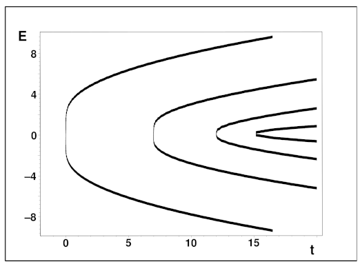
Far from the singular EP limits, i.e., in the middle of the separate open and disjunct non-EP intervals of $t\in (-\infty ,0)$, $t\in (0,7)$, $t\in (7,12)$, $t\in (12,15)$ and $t\in (15,\infty )$, the octuplet of the separate energy levels may be expected to be represented by the real or complex smooth functions of t. Numerically, such an expectation is strongly supported by Figure 1, in which we display all of the real eigenvalues of $H^{\left(8\right)}\left(t\right)$ as the functions of t in the interval ranging from the small negative values up to the $t>16$ domain of full Hermiticity. In the picture, one only has to notice that in the interval of $t\in (15,16)$ characterized by the full reality of the spectrum, the Hamiltonian itself still remains non-Hermitian. In the language of physicists [5], one could speak there about the dynamical regime with unbroken $\mathcal{PT}$-symmetry.

7. Summary

In our paper, we felt motivated by the recent enormous growth of intensity of the study of the quantum dynamical systems living near the EP singularities [56]. These studies are currently opening a comparatively new domain of quantum physics in which the challenging nature of the experiments is paralleled by the equally challenging nature of the necessary amendments of the conventional mathematical tools in functional analysis [57].

In the latter context, it is necessary to emphasize that the number of the newly emerging technical and conceptual difficulties is enormous [9]. At the same time, the existence of several specific features of the mathematics of non-Hermitian operators (cf. the dedicated monograph [9]) appears to have opened several new and promising directions of research in quantum mechanics (cf., e.g., the inspiring older review [5]). Briefly, one can say that at present, the experimental implementations of such an inspiration may be mostly found materialized in the quantum physics and phenomenology of the various forms of open systems [56]. In parallel, the progress in mathematics hitherto appeared more needed, relevant and productive in the closed-system applications. In this sense, our present paper offers a constructive (i.e., algebraic and perturbation-theoretic) mathematical, toy-model-based insight and support of the merits in both of these branches of the use of the updated non-Hermitian quantum theory.

Within the whole, fairly broad area of the related research, we decided to restrict our attention to the special and fairly provocative questions asked by Jones [11,45]. These questions were originally aimed at the illustrations of the specific methodical merits of the QHQM approach, and in particular, at the ability of the upgraded formalism to offer a deeper understanding of the widely studied phenomena of interference between the Hermitian and non-Hermitian components of various quantum systems in the laboratory.

In our paper, we managed to find several interesting and methodically encouraging answers to these questions. We revealed, in particular, that one may expect the existence of an intimate connection between the random or purposeful separation of the system into its weakly interacting (i.e., both Hermitian and non-Hermitian) components and the occurrence of its global non-Hermitian degeneracies.

The difficulty of the general answers to similar questions reflects one of the most influential currently existing terminological ambiguities, namely, the tendency of treating the closed quantum systems and open quantum systems more or less on the same footing. One of the consequences is that the mathematically correct and rigorous theorems may be accompanied by their misleading phenomenological applications. As a typical illustrative example, let us recall the concept of pseudospectrum [8]. Naturally, such a concept is perfectly suitable, say, for the analysis of stability in the open quantum systems, which are characterized by the plainly non-Hermitian Hamiltonians $H\ne H^{†}$ with the complex spectra of resonances [15]. At the same time, the description of the properties of the pseudospectra is much more difficult for the closed systems. Indeed, as long as the evolution of the latter systems is controlled by the quasi-Hermitian Hamiltonians $H\ne H^{†}$ (i.e., one must also re-construct the correct physical inner product metric $\Theta$ [6]), even the specialists in the full-fledged functional analysis find the task prohibitively difficult [58].

For this reason, the scope of our present study of the EP-related phenomena was restricted to the “toy-model” quantum systems for which the dimension N of all of the relevant Hilbert spaces remains finite. The price to pay was that we had to leave many currently studied questions (often motivated by the urgent methodical needs of the relativistic quantum field theory [5,7,13]) simply unnoticed. At the same time, a decisive benefit of the choice of $N<\infty$ is that it is very easy to distinguish between the models of the closed quantum systems (in which the spectra are easily tested to be real) and their open-system generalizations, for which the EP singularities are not only experimentally detectable but also mathematically richer.

In the theoretical part of our paper, we had to recall some of the known results in the EP-related perturbation theory. We re-emphasized that the basic mathematical difference emerges again between the open- and closed-system dynamical regimes. This observation enabled us to explain why, in the unitary, closed-system scenario requiring real spectrum, the construction of the admissible unfolding path in the space of parameters near the EP singularity must be fine-tuned. In the generic, open-system physical scenarios, on the contrary, it makes sense to study all of the complex forms of the spectra.

In the constructive part of our paper, the observation of the genericity of the complex EP(N)-unfolding patterns was supported by a remarkable one-parametric family of illustrative, EP-possessing “solvable” toy-model Hamiltonians $H^{\left(N\right)}\left(t\right)$. The model appeared, at any finite Hilbert-space dimension $N=2J$, exact and non-numerical, possessing a sequence of the EPs characterized by a decreasing degree of degeneracy corresponding to the equally quickly decreasing dimension of the non-Hermitian submatrix component C of the Hamiltonian.

References

- Messiah, A. Quantum Mechanics; North Holland: Amsterdam, The Netherlands, 1961. [Google Scholar]
- Stone, M.H. On one-parameter unitary groups in Hilbert Space. Ann. Math. 1932, 33, 643–648. [Google Scholar] [CrossRef]
- Dieudonne, J. Quasi-Hermitian Operators. In Proceedings of International Symposium on Linear Spaces; Pergamon: Oxford, UK, 1961; pp. 115–122. [Google Scholar]
- Scholtz, F.G.; Geyer, H.B.; Hahne, F.J.W. Quasi-Hermitian Operators in Quantum Mechanics and the Variational Principle. Ann. Phys. (NY) 1992, 213, 74–101. [Google Scholar] [CrossRef]
- Bender, C.M. Making sense of non-Hermitian Hamiltonians. Rep. Prog. Phys. 2007, 70, 947–1118. [Google Scholar] [CrossRef] [Green Version]
- Mostafazadeh, A. Pseudo-Hermitian Representation of Quantum Mechanics. Int. J. Geom. Meth. Mod. Phys. 2010, 7, 1191–1306. [Google Scholar] [CrossRef] [Green Version]
- Bender, C.M. PT Symmetry in Quantum and Classical Physics; World Scientific: Singapore, 2018. [Google Scholar]
- Trefethen, L.N.; Embree, M. Spectra and Pseudospectra; Princeton University Press: Princeton, NJ, USA, 2005. [Google Scholar]
- Bagarello, F.; Gazeau, J.-P.; Szafraniec, F.; Znojil, M. (Eds.) Non-Selfadjoint Operators in Quantum Physics: Mathematical Aspects; Wiley: Hoboken, NJ, USA, 2015. [Google Scholar]
- Krejčiřík, D.; Siegl, P.; Tater, M.; Viola, J. Pseudospectra in non-Hermitian quantum mechanics. J. Math. Phys. 2015, 56, 103513. [Google Scholar] [CrossRef] [Green Version]
- Jones, H.F. Coupling the Hermitian and Pseudo-Hermitian Worlds. (Transparencies of the Conference Talk on July 16, 2007, Available via the PHHQP Webpage). Available online: http://www.staff.city.ac.uk/~fring/PT (accessed on 20 July 2022).
- Jones, H.F. Scattering from localized non-Hermitian potentials. Phys. Rev. D 2007, 76, 125003. [Google Scholar] [CrossRef] [Green Version]
- Bender, C.M.; Jones, H.F. Interactions of Hermitian and non-Hermitian Hamiltonians. J. Phys. A Math. Theor. 2008, 41, 244006. [Google Scholar] [CrossRef] [Green Version]
- Znojil, M. Discrete PT-symmetric models of scattering. J. Phys. A Math. Theor. 2008, 41, 292002. [Google Scholar] [CrossRef] [Green Version]
- Moiseyev, N. Non-Hermitian Quantum Mechanics; CUP: Cambridge, UK, 2011. [Google Scholar]
- Feshbach, H. Unified theory of nuclear reactions. J. Ann. Phys. (NY) 1958, 5, 357–390. [Google Scholar] [CrossRef]
- Kato, T. Perturbation Theory for Linear Operators; Springer: Berlin/Heidelberg, Germany, 1966. [Google Scholar]
- Berry, M.V. Physics of Nonhermitian Degeneracies. Czechosl. J. Phys. 2004, 54, 1039–1047. [Google Scholar] [CrossRef]
- Heiss, W.D. Exceptional points—Their universal occurrence and their physical significance. Czechosl. J. Phys. 2004, 54, 1091–1100. [Google Scholar] [CrossRef]
- Klaiman, S.; Günther, U.; Moiseyev, N. Visualization of Branch Points in P T -Symmetric Waveguides. Phys. Rev. Lett. 2008, 101, 080402. [Google Scholar] [CrossRef] [PubMed] [Green Version]
- Borisov, D.I. Eigenvalues collision for PT-symmetric waveguide. Acta Polytech. 2014, 54, 93. [Google Scholar] [CrossRef]
- Teimourpour, M.H.; Zhong, Q.; Khajavikhan, M.; El-Ganainy, R. Higher Order EPs in Discrete Photonic Platforms. In Parity-Time Symmetry and Its Applications; Christodoulides, D., Yang, J.-K., Eds.; Springer: Singapore, 2018; pp. 261–276. [Google Scholar]
- Goldberg, A.Z.; Al-Qasimi, A.; Mumford, J.; O’Dell, D.H.J. Emergence of singularities from decoherence: Quantum catastrophes. Phys. Rev. A 2019, 100, 063628. [Google Scholar] [CrossRef] [Green Version]
- Ramirez, R.; Reboiro, M.; Tielas, D. Exceptional Points from the Hamiltonian of a hybrid physical system: Squeezing and anti-Squeezing. Eur. Phys. J. D 2020, 74, 193. [Google Scholar] [CrossRef]
- Znojil, M. Passage through exceptional point: Case study. Proc. Roy. Soc. A Math. Phys. Eng. Sci. 2020, 476, 20190831. [Google Scholar] [CrossRef] [Green Version]
- Guenther, U.; Stefani. F. IR-truncated PT -symmetric ix3 model and its asymptotic spectral scaling graph. arXiv 2019, arXiv:1901.08526. [Google Scholar]
- Semorádová, I.; Siegl, P. Diverging eigenvalues in domain truncations of Schroedinger operators with complex potentials. SIAM J. Math. Anal. 2022, in print. arXiv:2107.10557. [Google Scholar]
- Znojil, M. Quantum catastrophes: A case study. J. Phys. A Math. Theor. 2012, 45, 444036. [Google Scholar] [CrossRef] [Green Version]
- Zeeman, E.C. Cxatastrophe Theory-Selected Papers 1972–1977; Addison-Wesley: Reading, UK, 1977. [Google Scholar]
- Arnold, V.I. Catastrophe Theory; Springer: Berlin, Germany, 1992. [Google Scholar]
- Mostafazadeh, A. Hilbert space structures on the solution space of Klein-Gordon type evolution equations. Class. Quant. Grav. 2003, 20, 155–171. [Google Scholar] [CrossRef] [Green Version]
- Znojil, M. Relativistic supersymmetric quantum mechanics based on Klein-Gordon equation. J. Phys. A Math. Gen. 2004, 37, 9557–9571. [Google Scholar] [CrossRef] [Green Version]
- Mostafazadeh, A. Quantum mechanics of Klein-Gordon-type fields and quantum cosmology. Ann. Phys. (N.Y.) 2004, 309, 1–48. [Google Scholar] [CrossRef]
- Znojil, M. Wheeler–DeWitt equation and the applicability of crypto-Hermitian interaction representation in quantum cosmology. Universe 2022, 8, 385. [Google Scholar] [CrossRef]
- Znojil, M.; Borisov, D.I. Arnold’s potentials and quantum catastrophes II. Ann. Phys. 2022, 442, 168896. [Google Scholar] [CrossRef]
- Eremenko, A.; Gabrielov, A. Analytic continuation of eigenvalues of a quartic oscillator. Comm. Math. Phys. 2009, 287, 431. [Google Scholar] [CrossRef] [Green Version]
- Bender, C.M.; Wu, T.T. Anharmonic oscillator. Phys. Rev. 1969, 184, 1231. [Google Scholar] [CrossRef]
- Bender, C.M.; Boettcher, S. Real Spectra in Non-Hermitian Hamiltonians Having PT Symmetry. Phys. Rev. Lett. 1998, 80, 5243. [Google Scholar] [CrossRef] [Green Version]
- Siegl, P.; Krejčiřík, D. On the metric operator for the imaginary cubic oscillator. Phys. Rev. D 2012, 86, 121702(R). [Google Scholar] [CrossRef] [Green Version]
- Caliceti, E.; Graffi, S.; Maioli, M. Perturbation theory of odd anharmonic oscillators. Commun. Math. Phys. 1980, 75, 51. [Google Scholar] [CrossRef]
- Bessis, D. (IPN, Saclay, France). Private communication. 1992. [Google Scholar]
- Alvarez, G. Bender-Wu branch points in the cubic oscillator. J. Phys. A Math. Gen. 1995, 28, 4589–4598. [Google Scholar] [CrossRef]
- Znojil, M. Three-Hilbert-space formulation of Quantum Mechanics. Symmetry Integ. Geom. Meth. Appl. SIGMA 2009, 5, 1. [Google Scholar] [CrossRef]
- Alase, A.; Karuvade, S.; Scandolo, C.M. The operational foundations of PT-symmetric and quasi-Hermitian quantum theory. J. Phys. A Math. Theor. 2022, 55, 244003. [Google Scholar] [CrossRef]
- Jones, H.F. Interface between Hermitian and non-Hermitian Hamiltonians in a model calculation. Phys. Rev. D 2008, 78, 065032. [Google Scholar] [CrossRef] [Green Version]
- Znojil, M. Scattering theory using smeared non-Hermitian potentials. Phys. Rev. D 2009, 80, 045009. [Google Scholar] [CrossRef]
- Znojil, M. Exceptional points and domains of unitarity for a class of strongly non-Hermitian real-matrix Hamiltonians. J. Math. Phys. 2021, 62, 052103. [Google Scholar] [CrossRef]
- Znojil, M. Maximal couplings in PT-symmetric chain-models with the real spectrum of energies. J. Phys. A Math. Theor. 2007, 40, 4863–4875. [Google Scholar] [CrossRef] [Green Version]
- Znojil, M. Tridiagonal PT-symmetric N N Hamiltonians Afine-Tuning Their Obs. Domains Stronglynon-Hermitian Regime. J. Phys. A Math. Theor. 2007, 40, 13131–13148. [Google Scholar] [CrossRef] [Green Version]
- Buslaev, V.; Grecchi, V. Equivalence of unstable anharmonic oscillators and double wells. J. Phys. A Math. Gen. 1993, 26, 5541–5549. [Google Scholar] [CrossRef]
- Albeverio, S.; Kuzhel, S. PT-symmetric operators in quantum mechanics: Krein spaces methods. In Non-Selfadjoint Operators in Quantum Physics: Mathematical Aspects; Bagarello, F., Gazeau, J.-P., Szafraniec, F., Znojil, M., Eds.; Wiley: Hoboken, NJ, USA, 2015. [Google Scholar]
- Char, B.W.; Geddes, K.O.; Gonnet, G.H.; Leong, B.L.; Monagan, M.B.; Watt, S.M. Maple V; Springer: New York, NY, USA, 1991. [Google Scholar]
- Znojil, M. Unitary unfoldings of Bose-Hubbard exceptional point with and without particle number conservation. Proc. Roy. Soc. A Math. Phys. Eng. Sci. A 2020, 476, 20200292. [Google Scholar] [CrossRef] [PubMed]
- Znojil, M. Admissible perturbations and false instabilities in PT-symmetric quantum systems. Phys. Rev. A 2018, 97, 032114. [Google Scholar] [CrossRef] [Green Version]
- Znojil, M. Unitarity corridors to exceptional points. Phys. Rev. A 2019, 100, 032124. [Google Scholar] [CrossRef]
- Christodoulides, D.; Yang, J.-K. (Eds.) Parity-Time Symmetry and Its Applications; Springer: Singapore, 2018. [Google Scholar]
- Krejčiřík, D.; Siegl, P. Elements of spectral theory without the spectral theorem. In Non-Selfadjoint Operators in Quantum Physics: Mathematical Aspects; Bagarello, F., Gazeau, J.-P., Szafraniec, F., Znojil, M., Eds.; Wiley: Hoboken, NJ, USA, 2015. [Google Scholar]
- Siegl, P. (Tech. Univ., Graz, Austria). Private communication. 2016. [Google Scholar]
Figure 1.
The numerically calculated unfoldings and smoothness of the real eigenvalues of our toy model .