
SaMfENet: Self-Attention Based Multi-Scale Feature Fusion Coding and Edge Information Constraint Network for 6D Pose Estimation

1
Guangxi Key Laboratory of Manufacturing System and Advanced Manufacturing Technology, School of Electrical Engineering, Guangxi University, Nanning 530004, China
2
Guangxi Key Laboratory of Intelligent Control and Maintenance of Power Equipment, School of Electrical Engineering, Guangxi University, Nanning 530004, China
*
Author to whom correspondence should be addressed.
Mathematics 2022, 10(19), 3671; https://doi.org/10.3390/math10193671
Submission received: 21 August 2022
/
Revised: 30 September 2022
/
Accepted: 4 October 2022
/
Published: 7 October 2022
(This article belongs to the Special Issue Advances in Computer Vision and Machine Learning)
Abstract
:Accurate estimation of an object’s 6D pose is one of the crucial technologies for robotic manipulators. Especially when the lighting conditions changes or the object is occluded, resulting in the missing or the interference of the object information, which makes the accurate 6D pose estimation more challenging. To estimate the 6D pose of the object accurately, a self-attention-based multi-scale feature fusion coding and edge information constraint 6D pose estimation network is proposed, which can achieve accurate 6D pose estimation by employing RGB-D images. The proposed algorithm first introduces the edge reconstruction module into the pose estimation network, which improves the attention of the feature extraction network to the edge features. Furthermore, a self-attention multi-scale point cloud feature extraction module, i.e., MSPNet, is proposed to extract point cloud geometric features, which are reconstructed from depth maps. Finally, the clustering feature encoding module, i.e., SE-NetVLAD, is proposed to encode multi-modal dense feature sequences to construct more expressive global features. The proposed method is evaluated on the LineMOD and YCB-Video datasets, and the experimental results illustrate that the proposed method has an outstanding performance, which is close to the current state-of-the-art methods.
Keywords:
6D pose estimation; multi-scale feature fusion; attention mechanism; edge information constraintMSC:
68T071. Introduction
Six-dimensional pose estimation is of great significance for robotic grasping, augmented reality, autonomous driving, etc. However, the lighting condition variation and the occlusion of objects can make it extremely difficult for accurate 6D pose estimation.
Generally, the classical pose estimation methods can be roughly divided into two main categories for indoor environments. One kind of method is the corresponding feature points-based method, which establishes corresponding relationships between RGB image feature points and the 3D object model feature points; then the object pose can be calculated by applying the perspective-n-point (PnP) [1] algorithm. The other kind of method is a template matching-based method, which samples the 3D object point cloud model from multiple observation views to establish a template library. Then the image is matched with the templates in the template library to obtain the initial poses and perform subsequent optimization. Although traditional methods have many advantages, such as fast calculation, little amount of data required for training, etc., traditional methods cannot be applied in complex environments due to the weak robustness to disturbances, e.g., changes in illumination, occlusions, and the weak surface texture features of objects.
With the successful application of deep learning in computer vision, the application of deep learning in pose estimation has been researched and explored. This trend has led to the emergence of several data-driven 6D pose estimation methods, such as RGB data input-based networks, e.g., PVNet [2], BB8 [3], and PoseCNN [4], and RGB-D data input-based networks, e.g., DenseFusion [5] and PVN3D [6]. To a certain extent, the deep learning-based 6D pose estimation method has overcome the shortcomings of the above traditional methods. However, vulnerability to environmental disturbance cannot be eliminated easily. For instance, the PoseCNN employs an end-to-end approach to directly regress the 6D poses from RGB images. These methods have a greater advantage in calculating speed but generally have lower accuracy when the ambient lighting conditions are poor, or the object is occluded. With the inspiration of the traditional methods based on corresponding feature points, many methods, such as PVNet, have been proposed to calculate the 6D pose by locating feature points in the image. These methods exploit neural networks to predict feature points, which can improve the robustness significantly compared to traditional methods. However, these methods are still sensitive to influencing factors such as illumination changes and weak texture of the object.
Considering the above issues, the approaches to improving the 6D pose estimation network robustness are worth exploring and discussing. With the illumination condition changes, the stability of the object edge features has been clearly observed. Similarly, with weak object surface textures, there are still effective edge features that can be used for pose estimation. Nowadays, MaskedFusion [7], HybridPose [8], and several other approaches utilize mask or edge features in object 6D pose estimation. For example, MaskedFusion extends the DenseFusion network by employing the mask feature extraction branches. However, MaskedFusion simply adopts the same method for RGB images to the mask of the object. However, the complementary nature of the color and edge features are not emphasized, which leads to MaskedFusion still relying on iterative refinement to achieve high accuracy in pose estimation.
In addition, among the currently advanced methods, e.g., DenseFusion [5], MSCNet [9], and EANet [10], PointNet [11] is usually employed to extract the geometric features of the point cloud. However, PointNet only uses a single scale to extract the point cloud features, which loses the local geometric feature information of the point cloud. This leads to low accuracy pose estimation when the object is heavily occluded. Moreover, PointNet++ [12] is applied in PVN3D [6] to solve the loss of local geometric features of point clouds, while the complex structure of the PointNet++ network leads to slower forward inference in PVN3D.
The pose estimation methods such as DenseFusion and EANet usually use Maxpooling to extract global features of dense feature sequences. However, Maxpooling simply takes the maximum value in the dense feature sequence as the global feature, which ignores the distribution characteristics of the feature sequences. Additionally, the existence of outliers in the dense feature sequence may cause interference to the global features.
To solve the above problem, a novel 6D pose estimation network with edge feature constraints is proposed. To be more specific, texture features extracted by the network are used to perform edge reconstruction and calculate the edge reconstruction loss. Then, the combination of the edge reconstruction loss and the pose estimation loss contributes to optimizing the proposed network. The training phase for both the edge reconstruction and pose estimation tasks is conducted in the meantime. The increasing attention of the pose estimation network to edge features has been drawn by the edge reconstruction module; thereby the robustness to disturbances such as illumination changes has been dramatically improved. Meanwhile, to address the problem that PointNet extracts geometric features at a homogeneous scale, we propose the MSPNet, which is a multi-scale point cloud feature extraction network based on the self-attentiveness mechanism. Then we introduce the MSPNet into our pose estimation network for multi-scale feature extraction of point clouds obtained from depth image reconstruction. MSPNet adopts multiple parallel point cloud feature extraction modules to extract local geometric features at different scales and employs a self-attention mechanism to fuse the local geometric features from different scales.
To address the problem that Maxpooling has insufficient modeling capability and is susceptible to outlier interference, we propose the SE-NetVLAD, a clustered feature coding network. SE-NetVLAD clusters and encodes multi-modal dense feature sequences so that SE-NetVLAD is capable of extracting distributed features in feature sequences to construct more expressive global features. Finally, we further enhance the multi-modal dense feature sequences by reinforcing influential features and suppressing redundant features through a self-attention mechanism.
Our method has been evaluated on the LineMOD Dataset [13] and the YCB-Video Dataset [4]. The experiment results show that our method outperforms the advanced DenseFusion [5] with refinement by 0.7%, and our method has the best performance on smooth, untextured objects in the YCB-Video Dataset.
In summary, there are three main contributions of this work:
- We propose a self-attention-based multi-scale feature fusion coding and edge information constraint network for 6D pose estimation, named SaMfENet. The proposed network introduces an edge reconstruction module, which enhances the attention of the network to edge features. An accurate estimation of the object’s 6D pose can be achieved despite the changing effects of lighting conditions and the weak surface texture of the object.
- A self-attention multi-scale point cloud feature extraction network, named MSPNet, is proposed to extract local geometric features of point clouds at different scales and integrate features from different scales through the self-attention module. MSPNet can improve the 6D pose estimation accuracy with a few model parameters increasing.
- The clustered feature coding network, named SE-NetVLAD, is proposed to extract global features from multi-modal dense feature sequences. Compared to the maximum pooling layer, SE-NetVLAD is less sensitive to outlier interference and is capable of constructing more expressive global features.
The remainder of the article is organized as follows. Section 2 introduces the related works of pose estimation and attention mechanisms. Section 3 describes SaMfENet in detail. Section 4 describes experiments on LineMOD Dataset and YCB-Video Dataset and analyzes the experiment results. Finally, the conclusion of this article is given in Section 5.
Our code is open source, the code is available at https://github.com/r-9li/SaMfENet.
2. Related Work
2.1. Pose Estimation
The existing pose estimation methods can be mainly divided into traditional methods and deep learning-based methods. While traditional methods have a low tolerance to environmental disturbances and poor robustness, we, therefore, focus on 6D object pose estimation methods based on deep learning.
2.1.1. Pose Estimation from RGB Images
The 6D pose estimation methods based on RGB images extract the features of the image through the network and further return the 6D pose of the object. The direct regression method and the key point method are popular approaches for 6D pose estimation. The direct regression method uses the network to regress the object pose directly; for instance, PoseCNN [4] splits the 6D pose estimation task into three subtasks, namely semantic segmentation, 3D translation, and 3D rotation, then constructs a link between these three subtasks to make the network structure more reasonable. SSD-6D [14] extends the object detection task [15] to a 6D pose estimation task and abstracts the 3D rotation of an object to a discrete classification in space. The key point method involves predicting the projection of the object’s 3D key points on the 2D image through the network and then acquiring the object’s poses by the PnP algorithm. This method is more robust and faster than the direct regression method. In YOLO-6D [16], the object is detected by the YOLO [17] module at first, and the 2D projection of the 3D bounding box of the object is obtained, then the PnP algorithm is employed to solve the pose. Moreover, PVNet [2] extracts the features of the object through a convolutional neural network at the beginning and adopts pixel-level unit vector representation. These vectors are then voted on to determine the key points of the object, and the highest scoring key points are used to solve the poses.
Li et al. [18] proposed an iterative refinement method based on deep learning to estimate the 6D pose of objects called DeepIM. DeepIM optimizes the initial pose by minimizing the difference between the observed image and the rendered image. The iterative refinement process stops until the optimized pose converges or the number of iterations reaches a threshold. Further, Labbé et al. [19] proposed a more effective multi-object pose estimation method based on the idea of DeepIM, which is called CosyPose. They employed the rotation parametrization reported in [20] into CosyPose to make CNN training more stable.
Generally speaking, object 6D pose estimating methods based on RGB images have the advantages of simple input and fast processing. However, the neglect of spatial geometric information makes the estimation accuracy of these methods limited and less robust.
2.1.2. Pose Estimation from RGB-D Data
The current methods for pose estimation based on RGB-D images are mainly divided into three types. For the first type, depth information is utilized as additional information to optimize the estimation accuracy, e.g., PoseCNN [4], YOLO-6D [16], and BB8 [3]. These methods employ only RGB images to estimate the object pose roughly in the first stage, then generate point clouds based on depth information and RGB images. Finally, point cloud matching algorithms (e.g., Iterative Closest Point (ICP) [21], Generalized Iterative Closest Point (GICP) [22], and Super 4PCS [23]) are adopted to refine the object pose. For the second type, taking MCN [24] as an example, MCN splices the depth information channel with the RGB information channel and feeds the whole features into the network to predict the object pose. However, neither of these two types of methods deeply fuse RGB information with depth information, so these two types of methods cannot fully exploit the complementary nature of the two types of data. The use of point cloud matching algorithms such as ICP consumes a lot of time, which means these methods (e.g., PoseCNN + ICP, BB8 + ICP) cannot estimate the pose in real time.
By contrast, DenseFusion [5], MaskedFusion [7], and other methods have attempted to integrate RGB features deeply with depth-informed features at a later stage of feature extraction, which has achieved better results than the previous two types of methods. MSCNet [9] extends DenseFusion to extract further contextual information of point-level multi-modal features for enhancing feature expression ability after constructing those features. However, all of these methods only extract the geometric features of the point cloud at a single scale through PointNet, so the local geometric features of the point cloud are lost. Moreover, all of the above approaches focus on extracting color features of RGB images only, ignoring the importance of edge features in the pose estimation task.
To solve the above problem, a self-attention multi-scale point cloud feature extraction module, i.e., MSPNet, is proposed. At the same time, we incorporate the edge feature constraint into the pose estimation network and propose a self-attention-based multi-scale feature fusion coding and edge information constraint 6D pose estimation network.
2.2. Attention Mechanism
The attention mechanism was initially applied in machine translation [25,26,27], and now it has become an important part of neural networks. Many variants of attention mechanisms are widely used in computer vision and natural language processing tasks. For example, SENet [28] can learn the importance of each feature channel autonomously to activate practical features and suppress ineffective ones. ECANet [29] replaces the fully connected layer in SENet with a 1D convolutional layer, improving network performance dramatically with a small increase in the number of parameters and computation. GSoP-Net [30] extends SENet and replaces the global average pooling in SENet with second-order pooling, which compensates for the lack of modeling capability of global average pooling and makes GSoP-Net more capable of extracting global information.
Unlike the traditional convolutional layers with only one convolutional kernel, CondConv [31] assembles multiple convolutional kernels in one convolutional layer. Specifically, CondConv adopts a routing function to calculate the weight of each convolutional kernel based on the input to the convolutional layer and weighs each convolutional kernel by its weight. Finally, the weighted generated convolution kernel is used to convolve the input. CondConv achieves only a slight increase in computation while boosting model capacity and performs well on tasks such as image classification. SKNet [32] is capable of adjusting the receptive field of features adaptively by assigning weights to feature maps generated by convolution kernels of different sizes. Convolutional Block Attention Module (CBAM) [33] combines channel attention with spatial attention, which has excellent performance for improving the accuracy of object detection tasks.
Inspired by SKNet, the attention mechanism is introduced into MSPNet to integrate local features from different scales, avoiding significant increases in network parameters caused by high feature dimensionality.
3. The Proposed Method
The proposed network takes the RGB-D image as an input and outputs the 6D pose of the object. Specifically, the 6D pose of the object is the rigid transformation from the object coordinate system to the camera coordinate system. This rigid transformation is represented as a homogeneous transformation matrix consisting of a rotation transformation and a translation transformation .
3.1. Overview
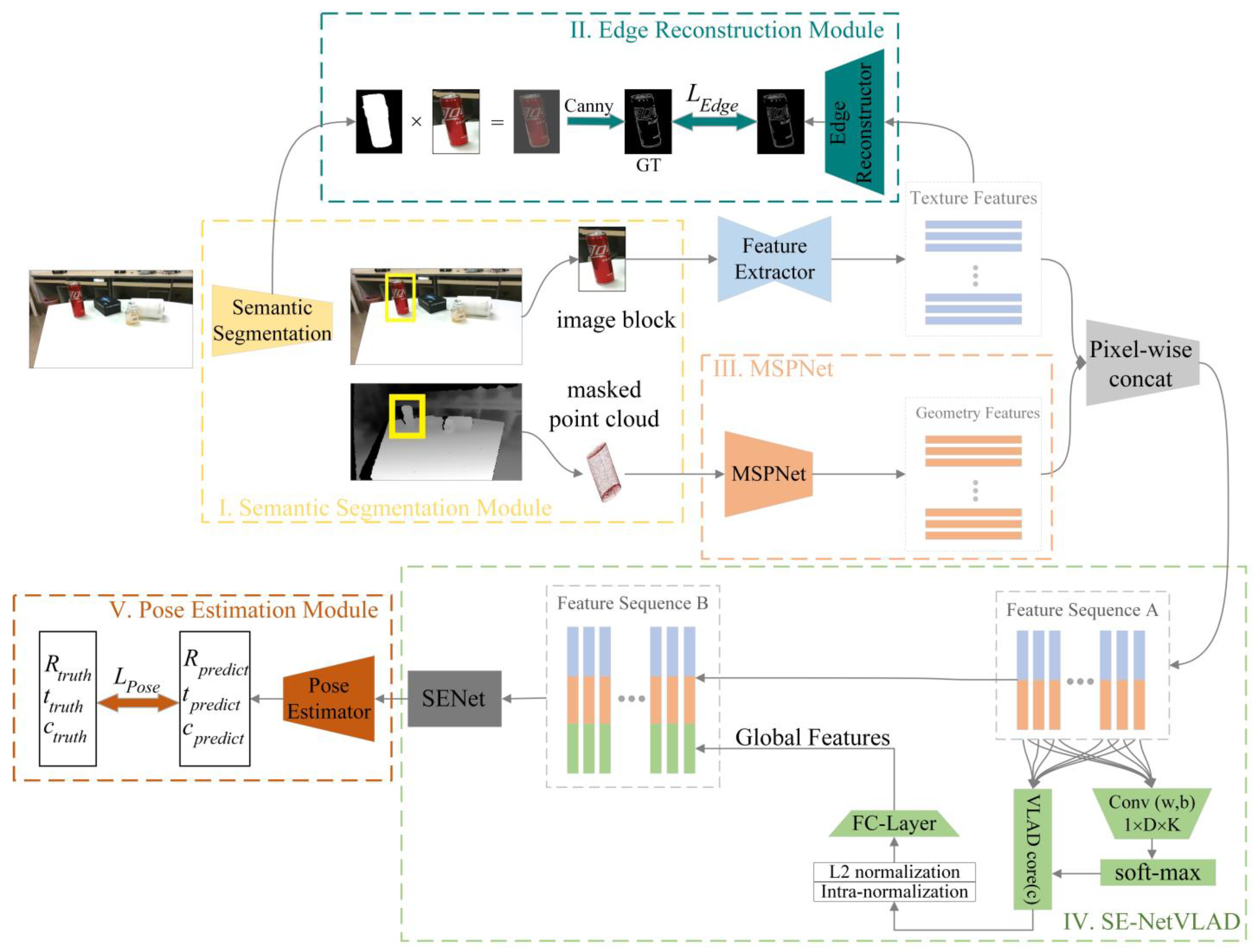
Figure 1 illustrates the overall architecture of SaMfENet. SaMfENet contains five main parts as follows:
- I. Semantic segmentation module. Based on the semantic segmentation network proposed in PoseCNN [4], the input RGB images are segmented to obtain a mask and bounding box for each instance object. The 3D point cloud is transformed from depth pixels covered by the mask, and the image block obtained by cropping with bounding boxes is used for subsequent feature extraction.
- II. Edge reconstruction module. The image block of the instance object is fed into an image feature extractor constructed via an encoder–decoder structure to extract the texture features. Then the edge reconstruction network generates an edge reconstruction image of the object based on the texture features. The object’s edges generated by the Canny [34] operator are used to constrain the edge reconstruction. It can improve the ability of image feature extraction to perceive edge information, thereby enhancing the robustness of the network to illumination changes.
- III. Multi-scale point cloud feature extraction module (MSPNet). The 3D point cloud reconstructed from the RGB-D image is fed into the MSPNet, which can extract the local geometric features of each point through multiple parallel Graph Conv Layers. Each Graph Conv Layer selects a different number of neighborhood points so that multiple parallel Graph Conv Layers can extract local geometric features at different scales. Finally, a self-attention mechanism is applied to fuse the local geometric features at different scales into a multi-scale geometric feature of the point cloud.
- IV. SE-NetVLAD for features fusion. The multi-modal dense feature sequence A constructed by pixel-wise texture features and geometric features are fed into SE-NetVLAD. Then, SE-NetVLAD constructs global features by clustering and encoding feature sequence A and concatenates the global features and feature sequence A at the pixel level. The influential features are further enhanced through a self-attention mechanism, while redundant features are suppressed.
- V. Pose estimation module. Feature sequence B is fed into the pose estimator, which consists of multiple consecutive convolutional layers. The pose estimator is used to perform regression translations and rotations directly.
3.2. Semantic Segmentation
In order to reduce the interference of the surrounding environment on the pose estimation, the object region should be segmented from the image first. In this work, the semantic segmentation network provided by PoseCNN is employed. The image semantic segmentation network constructed by an encoder–decoder structure takes an RGB image as input and outputs N + 1 binary maps. The activated pixels in each binary image indicate that these pixels belong to the object represented by the binary image. Based on the masks of the objects, we can obtain the bounding box that encloses these objects and crop the image with this bounding box to obtain the image block containing these objects. Moreover, the object regions in the depth map can be obtained by multiplying the masks of the objects and the depth map. Further, we transform the depth map into a visible surface point cloud of the object using the camera’s intrinsic parameters.
3.3. Edge-Attention Image Feature Extraction Module
3.3.1. Image Feature Extraction Module
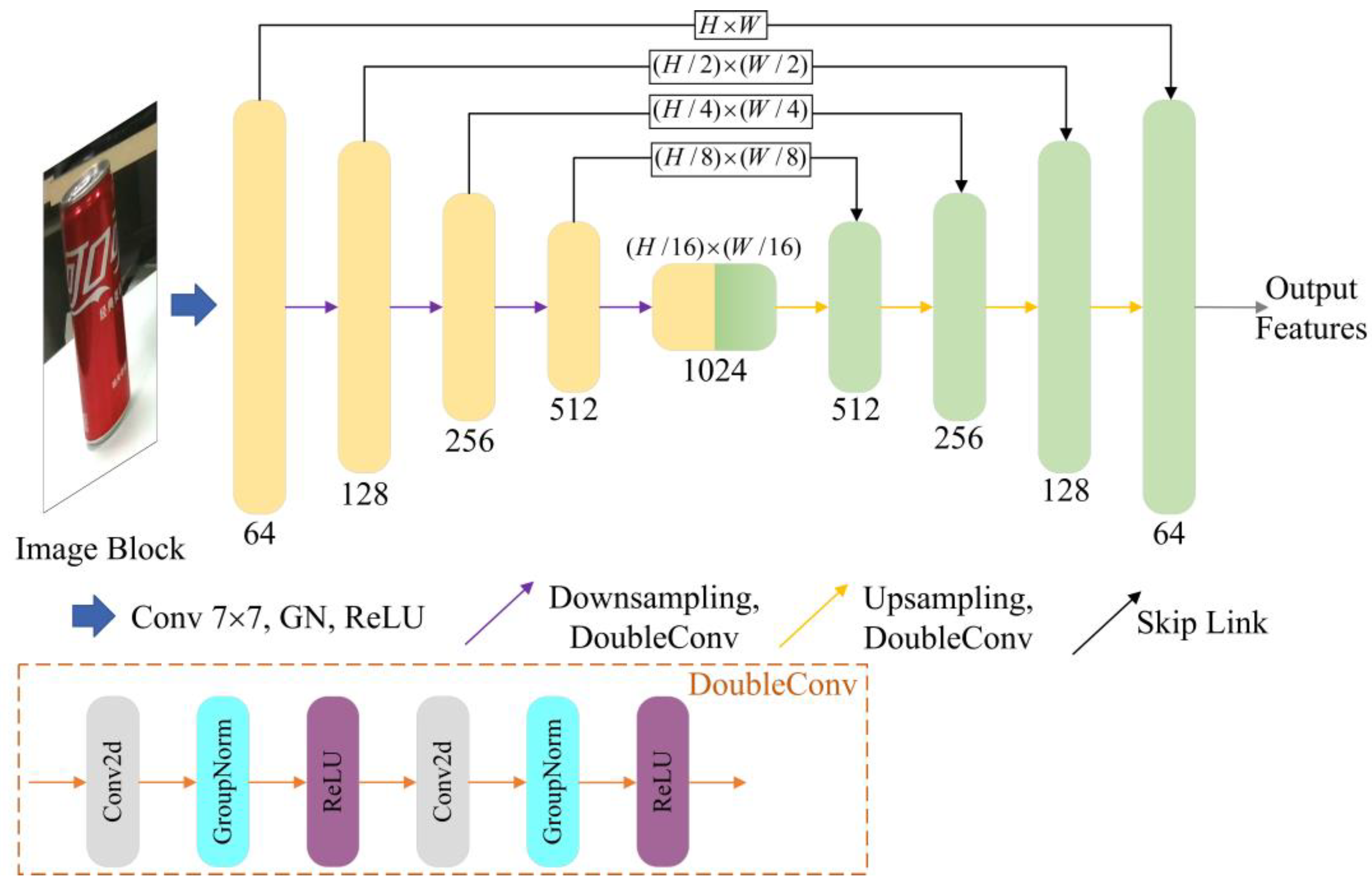
As the size of the cropped image blocks is not fixed, inspired by the property that the fully convolutional network (FCN) is not sensitive to the size of the input image, we designed an image feature extraction module that can be fed with images of arbitrary size. Although PSPNet [35] used in DenseFusion [5] can integrate features at different scales, the lack of shallow image features makes the output feature maps unfavorable for edge reconstruction. Therefore, an encoder–decoder network with a symmetric hourglass-type structure and a skip connection structure between the encoder and decoder is employed.
As shown in Figure 2, we first feed the image block into a 2D convolutional layer to generate a feature map with a size of (H, W, 64). This feature map is then fed into four successive downsampling modules to generate a feature map with a size of (H/16, W/16, 1024). The downsampling module includes two consecutive 2D convolutional layers (DoubleConv) and a maximum pooling layer. For the decoder part, we use four successive upsampling modules to recover the feature map with a size of (H/16, W/16, 1024) to a feature map with a size of (H, W, 64). The upsampling module consists of two consecutive 2D convolutional layers and a bilinear interpolation upsampling layer.
3.3.2. Edge Reconstruction Module
In real scene applications, the texture features of the object surface are easily affected by changes in ambient lighting. Moreover, the surface of some objects is smooth and weakly textured, which makes the texture-based feature extraction method ineffective. We observe that the edge features of the object surface remain stable when the lighting condition changes dramatically, and the objects with weak textures also have effective edge features for pose estimation. Therefore, the edge reconstruction module is designed. As shown in Figure 1(II), this module uses the Edge Reconstructor to generate an edge reconstruction image from the feature map output by the image feature extraction module. The Edge Reconstructor consists of two 1 × 1 convolutional layers, which can map the input feature map with the size of (H, W, 64) to an edge reconstruction image with the size of (H, W, 1). At the same time, we multiply the image block cropped by the bounding box with the mask of the object region to obtain an image block containing the object only. Moreover, we process this image block with the Canny [34] operator to generate the object edge for edge reconstruction.
The loss of the edge reconstruction task is defined as the binary cross-entropy (BCE), whose loss function can be expressed as:
where indicates the position of the pixel on the image,
indicates that pixel
is an edge pixel in the object edge,
represents the value of the pixel
in the edge reconstruction image, and
indicates the percentage of non-edge pixels to all pixels in the object edge.
3.4. Multi-Scale Point Cloud Geometric Feature Extraction Module
Typically, pose estimation methods do not fully exploit the complementary nature of depth information and RGB information. To solve this problem, we employ the depth image to generate the surface point cloud of the object and feed it into our network. Then the geometric features of the point cloud are extracted by a self-attention multi-scale point cloud feature extraction network, MSPNet. MSPNet extracts multi-scale geometric features of the point cloud through a parallel structure. Meanwhile, we introduce the self-attention mechanism into MSPNet to adaptively select the feature extraction scale.
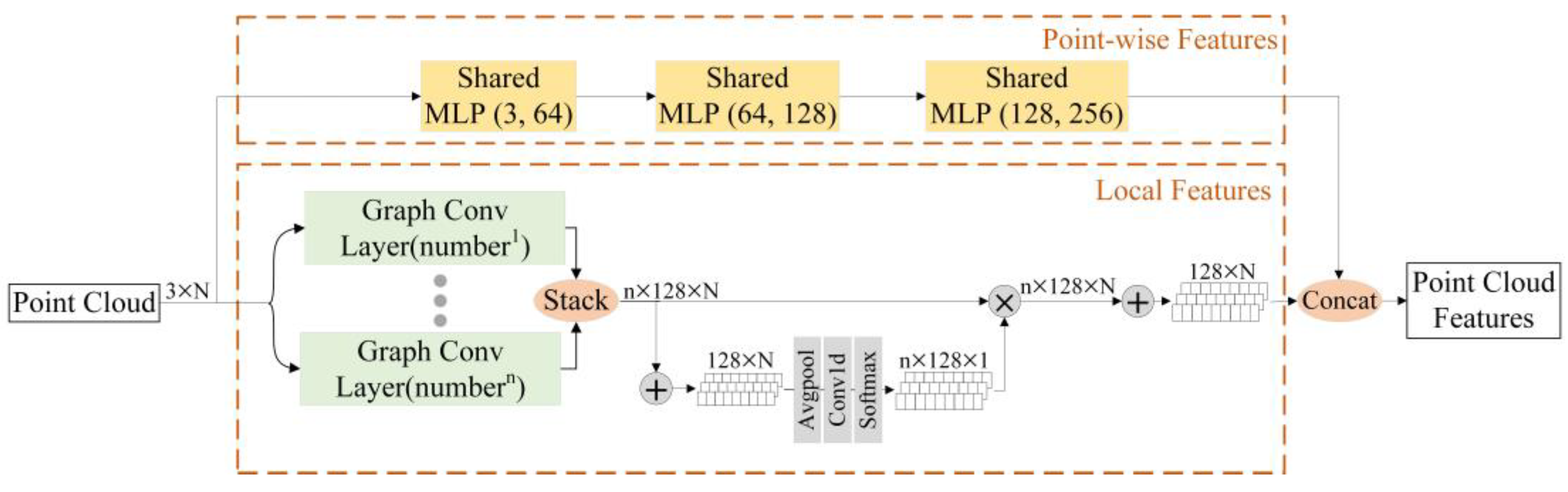
Figure 3 displays the specific process of our network for extracting geometric features. The network can be divided into two parts. The upper branch generates point-level features for each point by encoding the spatial location information of each point through three successive multi-layer perceptrons.
The lower branch aims to extract the local feature for the neighbors of each point. Multiple parallel Graph Conv Layers are employed to extract the local geometric features. Each Graph Conv Layer selects a different number of neighborhood points to extract local geometric features with multiple scales.
Figure 4 demonstrates the structure of the Graph Conv Layer. We first take each point as the center, then select the k nearest neighbor points with Euclidean distance and form a neighbor point set with the size of (3, k, N). Additionally, each point in the point cloud is subtracted by its k neighborhood points to generate a local feature vector with the size of (3, k, N), which is then mapped to a local feature vector with the size of (128, k, N) by a multi-layer perceptron. The process is expressed as:
where represents the i-th point, and
represents the j-th neighborhood point of the i-th point.
represents a non-linear function with parameters, i.e., a multi-layer perceptron.
Meanwhile, an attention mechanism is introduced to assign different weights to each point and its k neighborhood points. As shown in Figure 4, the self-coefficients obtained from the point cloud mapping represent the weights of each point, and the local-coefficients obtained from the local feature vector mapping represent the weights of the k neighborhood points of each point. We add the self-coefficients and local-coefficients to generate the final weight attention-coefficients . Then we multiply the local feature vector by the attention-coefficients with the size of (1, k, N) and then sum the result in the channel dimension to obtain the geometric features of the Graph Conv Layer output. The process can be expressed as:
where and represent different non-linear functions with parameters.
To allow the network to choose the scale for local features extraction adaptively, we introduce a self-attention mechanism after the feature extraction layer. Here, in order to obtain the weights of the feature vectors, we feed the sum of the feature vector output from the feature extraction layer into the network, which consists of the average pooling layer, the fully connected layer, and the softmax layer. The final output local feature vector is the result of the weighted summation of the feature vectors at each scale, which can be expressed as:
At last, the final geometric features are generated by concatenating the point-level features of each point with the local features.
3.5. Feature Fusion Module
3.5.1. Feature Fusion
In order to effectively fuse geometric and texture features, we used a pixel-level dense fusion strategy. This fusion strategy can avoid using a single global feature to estimate the object pose, thereby improving the robustness of the pose estimation network against inaccurate image segmentation or object occlusion. As shown in Figure 1(IV), the geometric features of each point are concatenated with the texture features to generate a multi-modal dense feature sequence.
3.5.2. Global Feature Extraction
Since the object is composed of multiple pixels, global features constructed by features of each pixel can be used to describe the object recapitulatively, which are essential for estimating object poses in a changing environment.
Here, we propose a SE-NetVLAD rather than the commonly used maximum pooling layer or average pooling layer to extract the global features of a feature sequence. Vector of Locally Aggregated Descriptors (VLAD) [36] was originally designed to aggregate local feature descriptors in an image into a global feature description vector. However, VLAD cannot be introduced into neural networks because it applies hard classification to find the nearest clustering center to the local feature descriptors. Hard classification means the neural network cannot optimize end-to-end by back-propagation. We replace the hard classification of local feature descriptors in VLAD with a differentiable soft classification, which allows SE-NetVLAD to be optimized end-to-end through back-propagation.
As shown in Figure 1(IV), the input to SE-NetVLAD is a one-dimensional multi-modal dense feature sequence with the size of (N, D), where D is the feature dimension. We first input the feature sequence into a 1 × 1 convolutional layer with a softmax layer to obtain the soft classification weights with the size of (N, K). can be expressed as:
Afterward, the soft classification weight is multiplied by the residual to obtain a feature vector with a size of (K, D), could be expressed as:
where is the number of clusters. and are the trainable parameter sets. We then reconstruct the feature vector into a 1D feature vector with size of (1, (K × D)), and feed it into a single fully connected layer to map it to a global feature vector. Finally, we concatenate the global feature vector with the multi-modal dense feature sequence at the pixel level to generate a multi-modal dense feature sequence containing the global features.
3.5.3. Self-Attention Mechanism
Multi-modal dense feature sequences may have redundant feature information, so we need to model the importance of feature channels explicitly and suppress redundant channels. Thus, we insert a channel attention module, as shown in Figure 1(IV). The feature sequence with the size of (N, D) is mapped to the channel weight vector with size of (1, D). The final output of the module, the feature sequence , is the weighting of on the original input feature sequence . can be expressed as:
3.6. 6D Object Pose Estimation
3.6.1. Pose Estimator
The pose estimator is composed of three parallel network structures, which are used to regress rotation, translation, and confidence. All three parallel network structures include four consecutive 1 × 1 convolutional layers. To make our method more robust for environmental changes and occlusion solutions, we regress a predicted pose for each feature vector in the multi-modal dense feature sequence. As shown in Figure 1(V), we input all feature vectors in the sequence into the pose estimator and generate a prediction for each feature vector. Meanwhile, we adopt a self-supervised method to select the best prediction, i.e., when the network returns to the pose, the confidence of the prediction result is regressed simultaneously. Among the dense prediction results, the prediction result with the highest confidence is selected as the final network output.
3.6.2. Loss Function
The proposed network model needs to learn the 6D poses of the object and the predicted confidence . In terms of the 6D pose estimation, we define the loss of pose estimation as the distance between the sample points on the object model after the ground truth and the predicted pose transformation. Therefore, the loss function of each dense prediction result is defined as follows:
where is the number of sample points on the 3D model of the object, is the j-th sampled point, is the ground truth, and is the i-th predicted pose.
The above loss function is only applicable to asymmetric objects, which have only one correct pose. While symmetrical objects may have more than one correct pose, still using the above loss function will result in the ambiguity of the object pose estimation. Therefore, for symmetrical objects, we define the loss of pose estimation as the distance between the sampled points on the object model after the ground truth and their nearest neighbor after the predicted pose transformation, where the loss function can be expressed as follows:
To make the network learn a confidence level for each prediction, we apply the confidence of the prediction results to weight the loss of the prediction results and add a confidence regularization term. The final pose estimation loss function can be expressed as:
where is the number of predicted outcomes and is a balanced hyperparameter.
Finally, we combine the edge reconstruction loss function and the pose estimation loss function as the final loss function with the hyperparameter , as shown in Equation (12).
4. Experiments
4.1. Datasets
To evaluate the performance of the proposed network, two open datasets (LineMOD Dataset [13] and YCB-Video Dataset [4]) are used to conduct experiments.
The LineMOD Dataset, which is well accepted to evaluate various classical or learning-based pose estimation methods, contains 13 weakly textured objects from 13 videos and does not contain synthetic images.
The YCB-Video Dataset consists of 92 videos containing a total number of 21 objects. Further, the YCB-Video Dataset contains distractions such as lighting condition changes and objects being occluded, which makes this dataset challenging.
4.2. Metrics
The accuracy of the pose estimation can be measured by two metrics, the average distance (ADD) and the average closest point distance (ADD-S).
The average distance is defined as the average distance between the sampling points on the object 3D model after the ground truth transformation and the sampling points after the predicted pose transformation, which can be expressed as:
where is the set of 3D model points and is the number of sample points.
The average closest point distance calculates the distance between the sampling points on the 3D model after the ground truth transformation and the closest point after the predicted pose transformation and then averages the distances between the closest points of all sampling points, which can be expressed as:
4.3. Implementation Details
Our method is implemented based on the PyTorch framework and adopts the Adam optimizer to optimize the network parameters at training time. All experiments in this work run on a desktop computer with an Intel® Xeon® E5-2680 v4 CPU and NVIDIA RTX 3090 2 GPUs. Within the process of training, we set the initial learning rate to 0.0001, the maximum number of iterations to 500, the number of sampling points to 1000, hyperparameter to 0.3, and hyperparameter to 0.015.
4.4. Evaluation on LineMOD Dataset
In the LineMOD Dataset, we consider the pose estimation to be correct if ADD-(S) (measured by ADD for asymmetric objects and ADD-S for symmetric objects) is lower than ten percent of the object diameter, which is the same as the previous work [5]. We use the percentage of correct key-frames for pose estimation to all key-frames to evaluate various methods. In addition, we refer to this percentage as accuracy in the following.
Table 1 shows the performance of our method and other state-of-the-art RGB-based or RGB-D-based methods on the LineMOD Dataset. From Table 1, the average accuracy of the RGB-based methods, such as BB8 (62.7%), PVNet (86.3%), PoseCNN + DeepIM (88.6%), and HRPose (91.6%), are lower than ours (95.0%), which is due to the fact that the RGB-based methods do not utilize spatial geometric information. When the ambient lighting conditions are not desirable or the surface texture of the object is weak (e.g., ape, duck), effective texture features cannot be extracted, resulting in inaccurate pose estimation. For the RGB-D-based method, SSD-6D + ICP only uses depth information in the post-processing stage without a deep fusion of texture features and geometric features, so the average accuracy of this method merely reaches 79%. EANet also exploits edge cues, but since our method uses MSPNet to extract multi-scale geometric features of point clouds and constructs more expressive dense feature sequences, our method outperforms EANet by 3.5% in the average accuracy. MSCNet uses multi-scale dense features for pose estimation, but since it does not use edge information to constrain the network, the pose estimation accuracy is lower when the object surface texture is weak, and the average accuracy is lower than our method by 0.4%.
We notice that keypoint-based methods (such as PVNet, HRPose) can achieve high pose estimation accuracy on bench can in the LineMOD Dataset. This is because bench and can have obvious texture features and geometric corners, so the keypoint-based methods can stably predict keypoints on bench. While our method does not exploit keypoints, it performs slightly worse on these two types of objects.
Moreover, we present the visualized results of our method on the LineMOD Dataset, which can be seen in Figure 5.
4.5. Evaluation of YCB-Video Dataset
Table 2 shows the pose estimation results on the YCB-Video Dataset. Two metrics are used to measure the effectiveness of the methods. One is the area under the ADD-S score-threshold curve (AUC), with thresholds ranging from 0 to 10 cm. Another indicator is the percentage of ADD-S scores of less than 2 cm (<2 cm). All methods use semantic segmentation masks from PoseCNN to guarantee fair comparison.
The experimental results illustrate that our method outperforms CosyPose, DenseFusion, MSCNet, and G2L-Net by 2.8%, 1.4%, 1.1%, and 0.2% on the first metric, respectively. The maximum error tolerated by robot grasping is 2 cm. Our method surpasses PoseCNN + ICP, DenseFusion, and MSCNet by 2.4%, 0.3%, and 1.7% in this metric, respectively. This proves that our method is more suitable for grasping tasks in the real world. An edge reconstruction module is introduced into the network, which implicitly improves the attention of the image feature extraction module to edge features, so our method shows the best performance on weakly textured objects such as banana, mug, and wood_block.
In the YCB-Video Dataset, large_clamp and extra_large_clamp are two types of objects with the same appearance but different sizes. Therefore, it is difficult for the semantic segmentation network provided by PoseCNN to generate the correct semantic segmentation masks for these two types of objects, which leads to poor performance of our network on large_clamp and extra_large_clamp. Moreover, scissors in the YCB-Video Dataset are small and have a discontinuous surface, so the edge-attention image feature extraction module cannot completely extract the texture features of scissors from the masked RGB images. Therefore, our network has lower pose estimation accuracy on scissors.
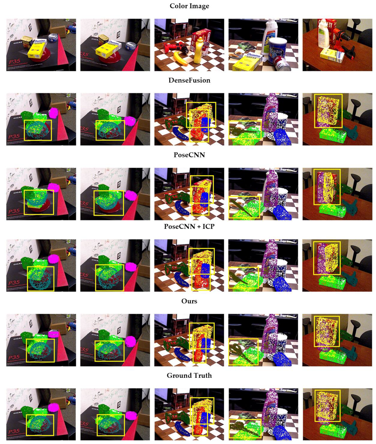
Figure 6 presents the qualitative analysis results of different methods on the YCB-Video Dataset. All methods use the semantic segmentation results provided by PoseCNN in this experiment. We transform the point cloud of the object according to the predicted 6D pose and project it onto a 2D image. The higher degree of coincidence between the transformed point cloud and the object means the higher accuracy of pose estimation. Our network predicts the results that have the highest degree of coincidence on smooth and textureless objects, such as bowl and banana. Conversely, DenseFusion and PoseCNN + ICP fail to accurately estimate the pose of the bowl and banana. This is because our method introduces edge information constraints into the pose estimation network, which improves the attention of our network to edge features and enables it to extract effective features for pose estimation even on smooth and texture-less objects. Because of the pixel-level prediction, our network also has a robust anti-occlusion capability and shows high prediction accuracy on the severely occluded cracker_box, scissors, and mustard_bottle.
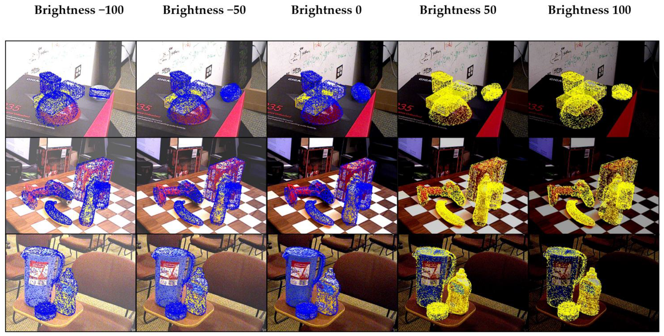
Figure 7 shows the performance of our method when the lighting condition changes. We randomly selected three images from the YCB-Video Dataset and then used the OpenCV to change the brightness of the images to simulate changes in illumination. From Figure 7, we can see that the pose estimation results hardly change with the brightness. This proves that our method is robust to lighting condition changes.
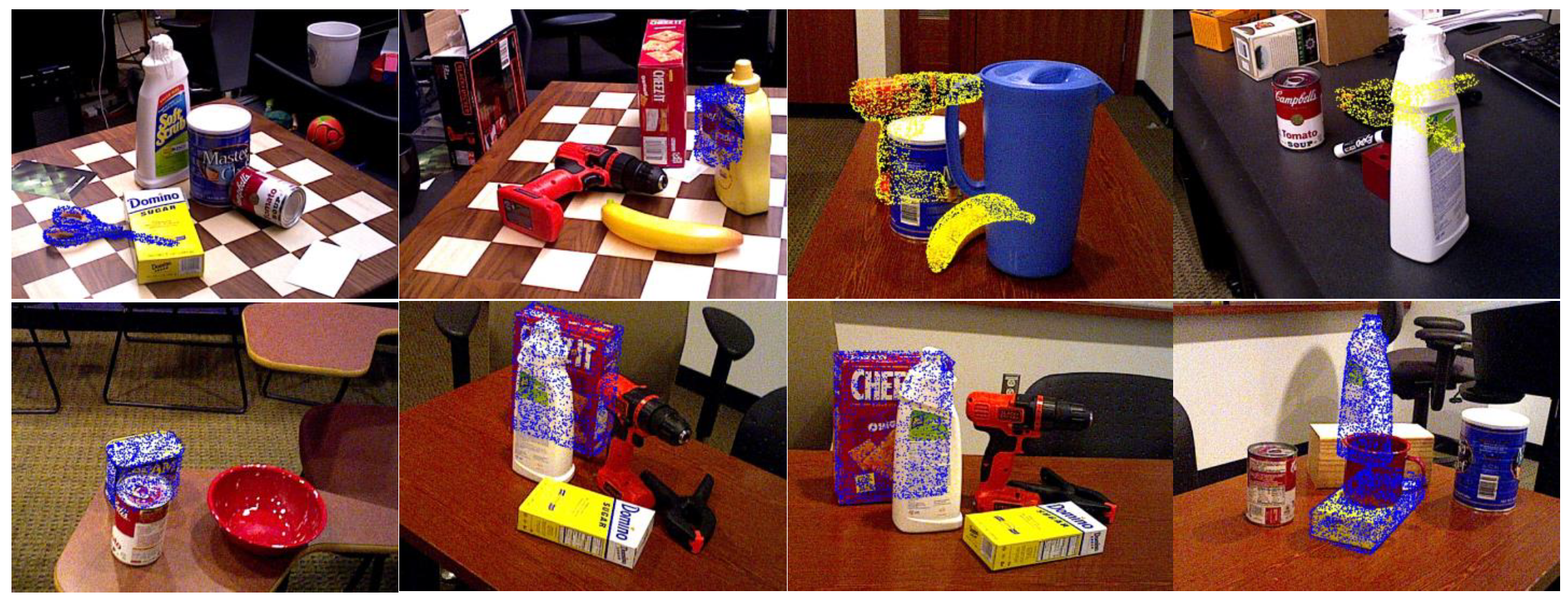
Figure 8 shows the performance of our method when the object is occluded. For a clearer presentation, we only render the pose estimation results of occluded objects on the graph. Figure 8 proves that our method can still estimate the 6D pose of the object accurately when the object is heavily occluded.
4.6. Ablation Study
All ablation experiments are performed on the LineMOD Dataset. The ablation study results are shown in Table 3, where the definition of accuracy is the same as the evaluation metric for the LineMOD Dataset. We test our improvement against DenseFusion [5] as a benchmark, i.e., model (a) represents DenseFusion without refinement. Based on DenseFusion, we employed the edge reconstruction module, MSPNet and SE-NetVLAD, forming model (b), model (c), and model (d), respectively. Model (d) represents our method.
Comparing model (a) and model (b), after the edge reconstruction module is introduced into the network, the pose estimation accuracy of model (b) is improved by 4.3%. This proves the edge reconstruction module can implicitly increase the attention of the image feature extraction module to edge features, thus improving the pose estimation performance. At the same time, we noticed that this multi-task learning training method could significantly improve the problem of difficulties in training the image feature extraction module because of the overall deep network and could also improve the speed of network convergence during training.
Comparing model (b) with model (c), model (b) uses PointNet to extract the geometric features of the reconstructed point cloud. While in model (c), we improved it to our proposed multi-scale point cloud feature extraction network MSPNet. Compared with model (b), the pose estimation accuracy of model (c) is improved by 3.4%, which proves that the multi-scale extraction of geometric features of point clouds can help improve the performance of pose estimation.
Similarly, the effectiveness of SE-NetVLAD can be verified by comparing model (c) and model (d). Table 3 shows that model (d) improves the pose estimation accuracy by 0.7% compared to model (c). Combining the above comparisons, we can find that each module proposed in our network makes a great contribution to improving the performance of pose estimation.
5. Conclusions
In this paper, we propose an end-to-end 6D pose estimation network based on RGB-D images, which was named SaMfENet. After a series of experiments, we prove the effectiveness of our method on the task of object 6D pose estimation. The proposed method can stably estimate the 6D pose of smooth, weak texture objects in complex lighting conditions. Our network is also robust to situations such as objects being severely occluded, meeting the needs of grasping tasks in the real scene. Moreover, ablation experiments prove that edge information constraints and multi-scale feature fusion can significantly improve pose estimation accuracy.
Our network is developed for real scene applications. In future work, we will apply our network to a robot to improve its performance in practical applications. Moreover, our network relies on a robust semantic segmentation network to segment object regions. However, using the independently trained semantic segmentation network, it is difficult to provide reliable and robust semantic segmentation results. In future work, we have a plan to deeply integrate the semantic segmentation network as a module into our network and train the semantic segmentation network together with the pose estimation network.
Author Contributions
Formal analysis, X.L.; Funding acquisition, Y.L.; Methodology, Z.L. and Y.L.; Software, Z.L.; Writing—original draft, Z.L.; Writing—review and editing, S.C., J.D. and Y.L. All authors have read and agreed to the published version of the manuscript.
Funding
This work was supported by the Guangxi Key Laboratory of Manufacturing System & Advanced Manufacturing Technology (Grant No. 20-065-40S005), the Key Laboratory of Advanced Manufacturing technology, Ministry of Education (Grant No. GZUAMT2021KF04), and the National College Students Innovation and Entrepreneurship Training Program (Grant No. 202110593003).
Institutional Review Board Statement
Not applicable.
Informed Consent Statement
Not applicable.
Data Availability Statement
Not applicable.
Conflicts of Interest
The authors declare no conflict of interest.
References
- Lepetit, V.; Moreno-Noguer, F.; Fua, P. Epnp: An accurate o (n) solution to the pnp problem. Int. J. Comput. Vis. 2009, 81, 155–166. [Google Scholar] [CrossRef] [Green Version]
- Peng, S.; Liu, Y.; Huang, Q.; Zhou, X.; Bao, H. Pvnet: Pixel-wise voting network for 6dof pose estimation. In Proceedings of the IEEE/CVF Conference on Computer Vision and Pattern Recognition, Padua, Italy, 18–23 July 2019; pp. 4561–4570. [Google Scholar]
- Rad, M.; Lepetit, V. Bb8: A scalable, accurate, robust to partial occlusion method for predicting the 3d poses of challenging objects without using depth. In Proceedings of the IEEE International Conference on Computer Vision, Venice, Italy, 22–29 October 2017; pp. 3828–3836. [Google Scholar]
- Xiang, Y.; Schmidt, T.; Narayanan, V.; Fox, D. Posecnn: A convolutional neural network for 6d object pose estimation in cluttered scenes. arXiv 2017, arXiv:1711.00199. [Google Scholar]
- Wang, C.; Xu, D.; Zhu, Y.; Martín-Martín, R.; Lu, C.; Fei-Fei, L.; Savarese, S. Densefusion: 6d object pose estimation by iterative dense fusion. In Proceedings of the IEEE/CVF Conference on Computer Vision and Pattern Recognition, Long Beach, CA, USA, 15–20 June 2019; pp. 3343–3352. [Google Scholar]
- He, Y.; Sun, W.; Huang, H.; Liu, J.; Fan, H.; Sun, J. Pvn3d: A deep point-wise 3d keypoints voting network for 6d of pose estimation. In Proceedings of the IEEE/CVF Conference on Computer Vision and Pattern Recognition, Seattle, WA, USA, 13–19 June 2020; pp. 11632–11641. [Google Scholar]
- Pereira, N.; Alexandre, L.A. MaskedFusion: Mask-based 6D object pose estimation. In Proceedings of the 2020 19th IEEE International Conference on Machine Learning and Applications (ICMLA), Miami, FL, USA, 14–17 December 2020; pp. 71–78. [Google Scholar]
- Song, C.; Song, J.; Huang, Q. Hybridpose: 6d object pose estimation under hybrid representations. In Proceedings of the IEEE/CVF Conference on Computer Vision and Pattern Recognition, Seattle, WA, USA, 13–19 June 2020; pp. 431–440. [Google Scholar]
- Gao, F.; Sun, Q.; Li, S.; Li, W.; Li, Y.; Yu, J.; Shuang, F. Efficient 6D object pose estimation based on attentive multi-scale contextual information. IET Comput. Vis. 2022, 16, 596–606. [Google Scholar] [CrossRef]
- Zhang, Y.; Liu, Y.; Wu, Q.; Zhou, J.; Gong, X.; Wang, J. EANet: Edge-attention 6D pose estimation network for texture-less objects. IEEE Trans. Instrum. Meas. 2022, 71, 1–13. [Google Scholar] [CrossRef]
- Qi, C.R.; Su, H.; Mo, K.; Guibas, L.J. Pointnet: Deep learning on point sets for 3d classification and segmentation. In Proceedings of the IEEE Conference On computer Vision and Pattern Recognition, Honolulu, HI, USA, 21–26 July 2017; pp. 652–660. [Google Scholar]
- Qi, C.R.; Yi, L.; Su, H.; Guibas, L.J. Pointnet++: Deep hierarchical feature learning on point sets in a metric space. Adv. Neural Inf. Process. Syst. 2017, 30, 5099–5108. [Google Scholar]
- Hinterstoisser, S.; Holzer, S.; Cagniart, C.; Ilic, S.; Konolige, K.; Navab, N.; Lepetit, V. Multimodal templates for real-time detection of texture-less objects in heavily cluttered scenes. In Proceedings of the 2011 International Conference on Computer Vision, Barcelona, Spain, 6–13 November 2011; pp. 858–865. [Google Scholar]
- Kehl, W.; Manhardt, F.; Tombari, F.; Ilic, S.; Navab, N. Ssd-6d: Making rgb-based 3d detection and 6d pose estimation great again. In Proceedings of the IEEE International Conference on Computer Vision, Venice, Italy, 22–29 October 2017; pp. 1521–1529. [Google Scholar]
- Liu, W.; Anguelov, D.; Erhan, D.; Szegedy, C.; Reed, S.; Fu, C.-Y.; Berg, A.C. Ssd: Single shot multibox detector. In Proceedings of the European Conference on Computer Vision, Amsterdam, The Netherlands, 11–14 October 2016; pp. 21–37. [Google Scholar]
- Tekin, B.; Sinha, S.N.; Fua, P. Real-time seamless single shot 6d object pose prediction. In Proceedings of the IEEE Conference on Computer Vision and Pattern Recognition, Salt Lake City, UT, USA, 18–23 June 2018; pp. 292–301. [Google Scholar]
- Redmon, J.; Divvala, S.; Girshick, R.; Farhadi, A. You only look once: Unified, real-time object detection. In Proceedings of the IEEE Conference on Computer Vision and Pattern Recognition, Las Vegas, NV, USA, 27–30 June 2016; pp. 779–788. [Google Scholar]
- Li, Y.; Wang, G.; Ji, X.; Xiang, Y.; Fox, D. Deepim: Deep iterative matching for 6d pose estimation. In Proceedings of the European Conference on Computer Vision (ECCV), Munich, Germany, 8–14 September 2018; pp. 683–698. [Google Scholar]
- Labbé, Y.; Carpentier, J.; Aubry, M.; Sivic, J. Cosypose: Consistent multi-view multi-object 6d pose estimation. In Proceedings of the European Conference on Computer Vision, Glasgow, UK, 23–28 August 2020; pp. 574–591. [Google Scholar]
- Zhou, Y.; Barnes, C.; Lu, J.; Yang, J.; Li, H. On the continuity of rotation representations in neural networks. In Proceedings of the IEEE/CVF Conference on Computer Vision and Pattern Recognition, Long Beach, CA, USA, 15–20 June 2019; pp. 5745–5753. [Google Scholar]
- Besl, P.J.; McKay, N.D. Method for registration of 3-D shapes. In Proceedings of the Sensor Fusion IV: Control Paradigms and Data Structures, Boston, MA, USA, 12–15 November 1992; pp. 586–606. [Google Scholar]
- Segal, A.; Haehnel, D.; Thrun, S. Generalized-icp. In Proceedings of the Robotics: Science and Systems, Seattle, WA, USA, 28 June–1 July 2009; p. 435. [Google Scholar]
- Mellado, N.; Aiger, D.; Mitra, N.J. Super 4pcs fast global pointcloud registration via smart indexing. Comput. Graph. Forum 2014, 33, 205–215. [Google Scholar] [CrossRef] [Green Version]
- Li, C.; Bai, J.; Hager, G.D. A unified framework for multi-view multi-class object pose estimation. In Proceedings of the European Conference on Computer Vision (ECCV), Munich, Germany, 8–14 September 2018; pp. 254–269. [Google Scholar]
- Vaswani, A.; Shazeer, N.; Parmar, N.; Uszkoreit, J.; Jones, L.; Gomez, A.N.; Kaiser, Ł.; Polosukhin, I. Attention is all you need. Adv. Neural Inf. Process. Syst. 2017, 30, 5998–6008. [Google Scholar]
- Bahdanau, D.; Cho, K.; Bengio, Y. Neural machine translation by jointly learning to align and translate. arXiv 2014, arXiv:1409.0473. [Google Scholar]
- Luong, M.-T.; Pham, H.; Manning, C.D. Effective approaches to attention-based neural machine translation. arXiv 2015, arXiv:1508.04025. [Google Scholar]
- Hu, J.; Shen, L.; Sun, G. Squeeze-and-excitation networks. In Proceedings of the IEEE Conference on Computer Vision and Pattern Recognition, Salt Lake City, UT, USA, 18–23 June 2018; pp. 7132–7141. [Google Scholar]
- Wang, Q.; Wu, B.; Zhu, P.; Li, P.; Zuo, W.; Hu, Q. Supplementary material for ‘ECA-Net: Efficient channel attention for deep convolutional neural networks. In Proceedings of the 2020 IEEE/CVF Conference on Computer Vision and Pattern Recognition, IEEE, Seattle, WA, USA, 13–19 June 2020; pp. 13–19. [Google Scholar]
- Gao, Z.; Xie, J.; Wang, Q.; Li, P. Global second-order pooling convolutional networks. In Proceedings of the IEEE/CVF Conference on Computer Vision and Pattern Recognition, Long Beach, CA, USA, 15–20 June 2019; pp. 3024–3033. [Google Scholar]
- Yang, B.; Bender, G.; Le, Q.V.; Ngiam, J. Condconv: Conditionally parameterized convolutions for efficient inference. Adv. Neural Inf. Process. Syst. 2019, 32, 1305–1316. [Google Scholar]
- Li, X.; Wang, W.; Hu, X.; Yang, J. Selective kernel networks. In Proceedings of the IEEE/CVF Conference on Computer Vision and Pattern Recognition, Long Beach, CA, USA, 15–20 June 2019; pp. 510–519. [Google Scholar]
- Woo, S.; Park, J.; Lee, J.-Y.; Kweon, I.S. Cbam: Convolutional block attention module. In Proceedings of the European Conference on Computer Vision (ECCV), Munich, Germany, 8–14 September 2018; pp. 3–19. [Google Scholar]
- Canny, J. A computational approach to edge detection. IEEE Trans. Pattern Anal. Mach. Intell. 1986, PAMI-8, 679–698. [Google Scholar] [CrossRef]
- Zhao, H.; Shi, J.; Qi, X.; Wang, X.; Jia, J. Pyramid scene parsing network. In Proceedings of the IEEE Conference on Computer Vision and Pattern Recognition, Honolulu, HI, USA, 21–26 July 2017; pp. 2881–2890. [Google Scholar]
- Jégou, H.; Douze, M.; Schmid, C.; Pérez, P. Aggregating local descriptors into a compact image representation. In Proceedings of the 2010 IEEE Computer Society Conference on Computer Vision and Pattern Recognition, San Francisco, CA, USA, 13–18 June 2010; pp. 3304–3311. [Google Scholar]
- Guan, Q.; Sheng, Z.; Xue, S. HRPose: Real-time high-resolution 6d pose estimation network using knowledge distillation. arXiv 2022, arXiv:2204.09429. [Google Scholar]
- Chen, W.; Jia, X.; Chang, H.J.; Duan, J.; Leonardis, A. G2l-net: Global to local network for real-time 6d pose estimation with embedding vector features. In Proceedings of the IEEE/CVF Conference on Computer Vision and Pattern Recognition, Seattle, WA, USA, 13–19 June 2020; pp. 4233–4242. [Google Scholar]
Figure 1.
The overall architecture of SaMfENet. SaMfENet can be divided into five parts. First, the input image is semantically segmented to obtain image blocks containing the object and the object point cloud reconstructed from the depth images. The image block is fed into the image feature extraction module to extract features afterward. We add edge feature constraints to improve the attention of the image feature extraction module to edge features. At the same time, the object point cloud is fed into MSPNet to extract the multi-scale geometric features of the point cloud. In addition, the two features emerged at the pixel level to obtain a multi-modal dense feature sequence, which is fed into SE-NetVLAD to extract the global features. Finally, the dense feature sequence is fed into the pose estimator to predict the rotation and translation.

Figure 2.
The structure of our image feature extraction module. The input of the module is an image block obtained by bounding box cropping, and the output is a feature map of the image block.
Figure 2.
The structure of our image feature extraction module. The input of the module is an image block obtained by bounding box cropping, and the output is a feature map of the image block.

Figure 3.
Structure of the multi-scale point cloud feature extraction network (MSPNet). The network can be divided into two parts, the upper part is the point-level feature extraction branch, while the lower part is the local feature extraction branch. The output features of the two branches are spliced as the geometric features of the point cloud. MLP is the abbreviation for multi-layer perceptron, and the numbers in brackets indicate the size of the layers.

Figure 4.
Structure of the Graph Conv Layer, where k is the number of the selected neighborhood points. MLP is the multi-layer perceptron, and the numbers in parentheses indicate the dimensions of the layers.
Figure 4.
Structure of the Graph Conv Layer, where k is the number of the selected neighborhood points. MLP is the multi-layer perceptron, and the numbers in parentheses indicate the dimensions of the layers.

Figure 5.
Visualization of results on the LineMOD Dataset.

Figure 6.
Qualitative results of the YCB-Video Dataset. The yellow box in the image shows that our method profoundly outperforms other methods on this object (from left to right: bowl, cracker_box, mustard_bottle, scissors, and cracker_box).
Figure 6.
Qualitative results of the YCB-Video Dataset. The yellow box in the image shows that our method profoundly outperforms other methods on this object (from left to right: bowl, cracker_box, mustard_bottle, scissors, and cracker_box).

Figure 7.
Visualized results of our method on the YCB-Video Dataset when lighting condition changes.
Figure 7.
Visualized results of our method on the YCB-Video Dataset when lighting condition changes.

Figure 8.
Visualized results of our method on the YCB-Video Dataset when objects are occluded.


Table 1.
Quantitative evaluation results on the LineMOD Dataset using the ADD-(S) metric, where the data shown in bold are the highest scores among different methods, and the objects marked with an asterisk * are symmetrical objects.
Table 1.
Quantitative evaluation results on the LineMOD Dataset using the ADD-(S) metric, where the data shown in bold are the highest scores among different methods, and the objects marked with an asterisk * are symmetrical objects.
| Input | RGB | RGB-D | |||||||
|---|---|---|---|---|---|---|---|---|---|
| Method | BB8 [3] | PVNet [2] | PoseCNN [4] + DeepIM [18] | HRPose [37] | SSD-6D [14] + ICP [21] | MSCNet [9] | DenseFusion [5] | EANet [10] | Ours |
| ape | 40.4 | 43.6 | 77.0 | 68.3 | 65.0 | 89.0 | 79.5 | 85.5 | 90.1 |
| bench | 91.8 | 99.9 | 97.5 | 99.4 | 80.0 | 93.1 | 84.2 | 92.2 | 91.0 |
| camera | 55.7 | 86.9 | 93.5 | 89.8 | 78.0 | 95.9 | 76.5 | 90.1 | 96.7 |
| can | 64.1 | 95.5 | 96.5 | 98.6 | 86.0 | 93.2 | 86.6 | 92.5 | 91.9 |
| cat | 62.6 | 79.3 | 82.1 | 90.0 | 70.0 | 95.0 | 88.8 | 93.0 | 96.4 |
| driller | 74.4 | 96.4 | 95.0 | 98.9 | 73.0 | 94.2 | 77.7 | 87.0 | 95.1 |
| duck | 44.3 | 52.6 | 77.7 | 72.7 | 66.0 | 90.3 | 76.3 | 79.9 | 90.8 |
| eggbox * | 57.8 | 99.2 | 97.1 | 100.0 | 100.0 | 100.0 | 99.9 | 99.7 | 99.8 |
| glue * | 41.2 | 95.7 | 99.4 | 98.7 | 100.0 | 100.0 | 99.4 | 98.9 | 99.7 |
| hole | 67.2 | 81.9 | 52.8 | 84.6 | 49.0 | 92.2 | 79.0 | 87.8 | 93.7 |
| iron | 84.7 | 98.9 | 98.3 | 99.0 | 78.0 | 96.5 | 92.1 | 94.8 | 97.9 |
| lamp | 76.5 | 99.3 | 97.5 | 99.4 | 73.0 | 95.1 | 92.3 | 95.7 | 96.6 |
| phone | 54.0 | 92.4 | 87.7 | 91.9 | 79.0 | 94.8 | 88.0 | 92.5 | 95.9 |
| Mean | 62.7 | 86.3 | 88.6 | 91.6 | 79.0 | 94.6 | 86.2 | 91.5 | 95.0 |
Table 2.
Quantitative evaluation results using the ADD-S metric on the YCB-Video Dataset, where the data shown in bold are the highest scores among the different methods, and the objects marked with an asterisk * are symmetrical objects.
Table 2.
Quantitative evaluation results using the ADD-S metric on the YCB-Video Dataset, where the data shown in bold are the highest scores among the different methods, and the objects marked with an asterisk * are symmetrical objects.
| Input | RGB | RGB-D | ||||||||||
|---|---|---|---|---|---|---|---|---|---|---|---|---|
| Methods | CosyPose [19] | PoseCNN [4] + ICP [21] | DenseFusion [5] | MSCNet [9] | G2L-Net [38] | Ours | ||||||
| AUC | <2 cm | AUC | <2 cm | AUC | <2 cm | AUC | <2 cm | AUC | <2 cm | AUC | <2 cm | |
| 002_master_chef_can | 92.6 | - | 95.8 | 100.0 | 95.2 | 100.0 | 94.7 | 96.0 | 94.0 | - | 95.9 | 100.0 |
| 003_cracker_box | 93.7 | - | 92.7 | 91.6 | 92.5 | 99.3 | 93.4 | 89.4 | 88.7 | - | 94.1 | 94.8 |
| 004_sugar_box | 96.6 | - | 98.2 | 100.0 | 95.1 | 100.0 | 95.7 | 100.0 | 96.0 | - | 97.2 | 100.0 |
| 005_tomato_soup_can | 92.5 | - | 94.5 | 96.9 | 93.7 | 96.9 | 94.1 | 96.7 | 86.4 | - | 94.2 | 96.9 |
| 006_mustard_bottle | 96.0 | - | 98.6 | 100.0 | 95.9 | 100.0 | 95.3 | 100.0 | 95.9 | - | 95.4 | 100.0 |
| 007_tuna_fish_can | 96.6 | - | 97.1 | 100.0 | 94.9 | 100.0 | 95.5 | 98.3 | 96.0 | - | 94.7 | 100.0 |
| 008_pudding_box | 80.8 | - | 97.9 | 100.0 | 94.7 | 100.0 | 94.4 | 99.0 | 93.5 | - | 95.9 | 100.0 |
| 009_gelatin_box | 97.0 | - | 98.8 | 100.0 | 95.8 | 100.0 | 97.6 | 100.0 | 96.8 | - | 97.3 | 100.0 |
| 010_potted_meat_can | 90.6 | - | 92.7 | 93.6 | 90.1 | 93.1 | 90.0 | 89.6 | 86.2 | - | 91.2 | 94.1 |
| 011_banana | 95.4 | - | 97.1 | 99.7 | 91.5 | 93.9 | 90.3 | 94.5 | 96.3 | - | 97.3 | 100.0 |
| 019_pitcher_base | 96.1 | - | 97.8 | 100.0 | 94.6 | 100.0 | 93.9 | 100.0 | 91.8 | - | 96.7 | 100.0 |
| 021_bleach_cleanser | 92.2 | - | 96.9 | 99.4 | 94.3 | 99.8 | 94.7 | 99.3 | 92.0 | - | 95.5 | 99.6 |
| 024_bowl * | 82.4 | - | 81.0 | 54.9 | 86.6 | 69.5 | 93.1 | 93.1 | 86.7 | - | 89.5 | 93.4 |
| 025_mug | 94.0 | - | 95.0 | 99.8 | 95.5 | 100.0 | 94.4 | 100.0 | 95.4 | - | 97.1 | 100.0 |
| 035_power_drill | 94.7 | - | 98.2 | 99.6 | 92.4 | 97.1 | 91.7 | 99.3 | 95.2 | - | 96.0 | 99.6 |
| 036_wood_block * | 78.3 | - | 87.6 | 80.2 | 85.5 | 93.4 | 90.3 | 98.8 | 86.2 | - | 91.1 | 99.2 |
| 037_scissors | 81.3 | - | 91.7 | 95.6 | 96.4 | 100.0 | 87.6 | 59.7 | 83.8 | - | 84.1 | 67.4 |
| 040_large_marker | 90.7 | - | 97.2 | 99.7 | 94.7 | 99.2 | 96.1 | 99.7 | 96.8 | - | 97.0 | 99.9 |
| 051_large_clamp * | 74.8 | - | 75.2 | 74.9 | 71.6 | 78.5 | 71.6 | 76.1 | 94.4 | - | 73.8 | 77.5 |
| 052_extra_large_clamp * | 78.5 | - | 64.4 | 48.8 | 69.0 | 69.5 | 68.2 | 61.7 | 92.3 | - | 67.6 | 66.1 |
| 061_foam_brick * | 92.0 | - | 97.2 | 100.0 | 92.4 | 100.0 | 95.1 | 100.0 | 94.7 | - | 95.5 | 100.0 |
| Mean | 89.8 | - | 93.0 | 93.2 | 91.2 | 95.3 | 91.5 | 93.9 | 92.4 | - | 92.6 | 95.6 |
Table 3.
Results of ablation experiments.
| Model | (a) | (b) | (c) | (d) |
|---|---|---|---|---|
| Edge Reconstruction Module | × | ✓ | ✓ | ✓ |
| MSPNet | × | × | ✓ | ✓ |
| SE-NetVLAD | × | × | × | ✓ |
| Accuracy | 86.2 | 90.5 | 93.9 | 94.6 |
Publisher’s Note: MDPI stays neutral with regard to jurisdictional claims in published maps and institutional affiliations. |
© 2022 by the authors. Licensee MDPI, Basel, Switzerland. This article is an open access article distributed under the terms and conditions of the Creative Commons Attribution (CC BY) license (https://creativecommons.org/licenses/by/4.0/).
Share and Cite
MDPI and ACS Style
Li, Z.; Li, X.; Chen, S.; Du, J.; Li, Y. SaMfENet: Self-Attention Based Multi-Scale Feature Fusion Coding and Edge Information Constraint Network for 6D Pose Estimation. Mathematics 2022, 10, 3671. https://doi.org/10.3390/math10193671
AMA Style
Li Z, Li X, Chen S, Du J, Li Y. SaMfENet: Self-Attention Based Multi-Scale Feature Fusion Coding and Edge Information Constraint Network for 6D Pose Estimation. Mathematics. 2022; 10(19):3671. https://doi.org/10.3390/math10193671
Chicago/Turabian StyleLi, Zhuoxiao, Xiaobing Li, Shihao Chen, Jialong Du, and Yong Li. 2022. "SaMfENet: Self-Attention Based Multi-Scale Feature Fusion Coding and Edge Information Constraint Network for 6D Pose Estimation" Mathematics 10, no. 19: 3671. https://doi.org/10.3390/math10193671
Note that from the first issue of 2016, this journal uses article numbers instead of page numbers. See further details here.