Article

Computational Analysis of XLindley Parameters Using Adaptive Type-II Progressive Hybrid Censoring with Applications in Chemical Engineering

1
Department of Mathematical Sciences, College of Science, Princess Nourah Bint Abdulrahman University, P.O. Box 84428, Riyadh 11671, Saudi Arabia
2
Department of Statistics, Faculty of Science, King Abdulaziz University, Jeddah 21589, Saudi Arabia
3
Department of Statistics, Faculty of Commerce, Zagazig University, Zagazig 44519, Egypt
4
Faculty of Technology and Development, Zagazig University, Zagazig 44519, Egypt
*
Author to whom correspondence should be addressed.
Mathematics 2022, 10(18), 3355; https://doi.org/10.3390/math10183355
Submission received: 27 July 2022 / Revised: 5 September 2022 / Accepted: 8 September 2022 / Published: 15 September 2022
(This article belongs to the Special Issue Advances in Computational Statistics and Applications)

Abstract

:
This work addresses the estimation issues of the XLindley distribution using an adaptive Type-II progressive hybrid censoring scheme. Maximum likelihood and Bayesian approaches are used to estimate the unknown parameter, reliability, and hazard rate functions. Bayesian estimators are explored under the assumption of independent gamma priors and a symmetric loss function. The approximate confidence intervals and the highest posterior density credible intervals are also computed. An extensive simulation study that takes into account various sample sizes and censoring schemes is implemented to evaluate the various estimating methods. Finally, for an explanation, two real data sets from the chemical engineering field are provided to show that the XLindley distribution is the best model compared to some competitive models for the same real data. The Bayesian paradigm utilizing the Metropolis–Hastings algorithm to generate samples from the posterior distribution is recommended to estimate any parameter of life of the XLindley distribution when data are obtained from adaptive Type-II progressively hybrid censored sample.

1. Introduction

Studies on reliability and life testing frequently use censored data. It is necessary for experimenters to gather data using censored samples for reasons including conserving the working experimental units for future use, decreasing the total time on the test, and financial constraints. The two censoring methods that are most commonly applied in life testing and reliability studies are time censoring (Type-I) and failure censoring (Type-II) schemes. These methods lack the flexibility to allow units to be withdrawn from the experiment at any point other than the terminal point. To avoid this disadvantage, a more flexible censoring scheme known as a progressive Type-II censoring scheme is introduced. Kundu and Joarder [1] suggested a progressive Type-I hybrid censoring scheme, in which n identical items are tested using a specified progressive censoring scheme R 1 , R 2 , · · · , R m and the test is ended at random time T * = m i n ( X m : m : n , T ) , where T is a predetermined time. This scheme has the disadvantage that the useful sample size is random and might be found to be a very small number or zero for reliable products. As a result, the statistical inference methods will be inefficient.
To overcome this drawback, Ng et al. [2] proposed an adaptive progressive Type-II hybrid censoring scheme to increase the efficiency of statistical analysis. The number of failures m is predetermined in advance in this scheme, and the testing time is permitted to run over the prefixed time T. Moreover, we have the progressive censoring scheme R 1 , R 2 , · · · , R m , but the values of some of the R i may be adjusted consequently during the test. This scheme can be described briefly as follows: Assume that n units are placed on a life test and m < n is the desired number of failures. At the time of the first failure X 1 : m : n , R 1 units are randomly removed from the test. Similarly, at the time of the second failure X 2 : m : n , R 2 units are randomly withdrawn from the test, and so on. If the m t h failure happens before time T ( i . e . , X m : m : m < T ) , the test stops at this time and we will have the usual progressive Type-II censoring. On the other hand, if X d : m : n < T < X d + 1 : m : n , where d + 1 < m and X d : m : n is the d t h failure time happen before time T, then we will not withdraw any surviving item from the test by putting R d + 1 , R d + 2 , · · · , R m 1 = 0 and R m * = n m i = 1 d R i . This setting allows us to end the test when we reach the preferred number of failures m, and the total test time will not be too far away from the ideal time T. Let x 1 : m : n < < x d : m : n < T < x d + 1 : m : n < < x m : m : n be an adaptive progressively Type-II hybrid censored sample from a continuous population with probability density function (PDF) f ( x ) and cumulative distribution function (CDF) F ( x ) with progressive censoring scheme R 1 , , R d , 0 , , 0 , R m * , then the likelihood function of the observed data can be expressed as follows
L = C i = 1 m f ( x i : m : n ) i = 1 d [ 1 F ( x i : m : n ) ] R i [ 1 F ( x m : m : n ) ] R m * ,
where C is a constant that is independent of the parameters. Various studies based on the adaptive progressive Type-II hybrid censoring scheme have been conducted. Hemmati and Khorram [3] studied the estimation problems of the exponential distribution in the presence of a competing risks model. Nassar and Abo-Kasem [4] investigated some estimation methods for the inverse Weibull distribution. Ateya and Mohammed [5] discussed the statistical inferences of the exponentiated exponential distribution. Nassar et al. [6,7] studied the estimation of Weibull and Rayleigh distributions, respectively. See also, Sobhi and Soliman [8], Panahi and Moradi [9], Chen and Gui [10], Panahi and Asadi [11], Okasha et al. [12] and Alotaibi et al. [13] among many others.
Furthermore, the Lindley distribution, first proposed by Lindley [14], has been used extensively in different areas of science and technology. It is an important statistical model for studying stress–strength reliability modeling. Recently, Chouia and Zeghdoudi [15] proposed a new modification version of the Lindley distribution, as a special mixture of exponential and Lindley distributions, called XLindley (XL) distribution. Suppose that X is a lifetime random variable of an experimental units follow XL with scale parameter λ . Hence, the corresponding PDF and CDF of X are given by
f ( x ; λ ) = λ 2 λ + x + 2 1 + λ 2 e λ x , x > 0 , λ > 0 ,
and
F ( x ; λ ) = 1 1 + λ x 1 + λ 2 e λ x , x > 0 , λ > 0 ,
respectively. The reliability characteristics of any lifetime model are the main features for evaluating the capacity of any electronic system that a reliability practitioner has frequently used.
Therefore, some reliability indices of the XL distribution can be also investigated as unknown parameters, namely, reliability function (RF) R ( · ) and hazard rate function (HRF) h ( · ) at distinct time t which can be given, respectively, by
R ( t ; λ ) = 1 + λ t 1 + λ 2 e λ t , t > 0 , λ > 0 ,
and
h ( t ; λ ) = λ 2 λ + t + 2 1 + λ 2 + λ t , t > 0 , λ > 0 .
The novelty of our study comes from the fact that it is the first to investigate the estimation issues of the XL distribution under the adaptive progressive Type-II hybrid censoring scheme. We can list the main objectives of this study as follows: (1) To obtain the maximum likelihood estimator (MLE) of the scale parameter λ , RFand HRF along with their approximate confidence intervals (ACIs). (2) To acquire the Bayesian estimators of the different parameters using the squared error loss (SEL) function as well as the associated highest posterior density (HPD) credible intervals. (3) To compare the efficiency of the various point and interval estimators through a simulation study. (4) To show the applicability of the offered methods via exploring two real data sets, and to see how the different proposed methods can work in real-life scenarios.
The rest of the article is structured as follows: Section 2 is devoted to discussing the MLEs and ACIs of the parameter, and RF and HRF for the the XL distribution. In Section 3, the Bayesian estimating method is discussed. The findings of a simulation investigation are presented in Section 4. Two real data sets are examined in Section 5, and the paper is concluded in Section 6.

2. Classical Inference

Let x 1 : m : n < < x d : m : n < T < x d + 1 : m : n < < x m : m : n be an adaptive progressively Type-II hybrid censored sample of size m with progressive censoring scheme R 1 , , R d , 0 , , 0 , R m from XL model. In this case, the likelihood function, ignoring the constant term, can be obtained from (1), (2) and (3), as follows
L ( λ ) = λ 1 + λ 2 m exp λ i = 1 m x i + i = 1 d R i x i + R m * x m + i = 1 m log ( λ + x i + 2 ) × i = 1 d 1 + λ x i ( 1 + λ ) 2 R i 1 + λ x m ( 1 + λ ) 2 R m * ,
where x i = x i : m : n , i = 1 , , m for simplicity. Let ( λ ) = log L ( λ ) be the log-likelihood function, then the MLE of the parameter λ , denoted by λ ^ , can be obtained by maximizing ( λ ) expressed as
( λ ) = 2 m log λ 1 + λ λ i = 1 m x i + i = 1 d R i x i + R m * x m + i = 1 m log ( λ + x i + 2 ) + i = 1 d R i log 1 + λ x i ( 1 + λ ) 2 + R m * log 1 + λ x m ( 1 + λ ) 2 ,
with respect to λ .
Instead of maximizing the objective function in (7), the MLE λ ^ can be acquired by solving the following nonlinear equation
d ( λ ) d λ = 2 m λ ( 1 + λ ) i = 1 m x i + i = 1 d R i x i + R m * x m + i = 1 m ( λ + x i + 2 ) 1 + 1 λ 1 + λ i = 1 d R i x i [ 1 + λ ( λ + x i + 2 ) ] 1 + 1 λ 1 + λ R m * x m [ 1 + λ ( λ + x m + 2 ) ] 1 = 0 .
One can see from (8) that there is no closed form for the MLE λ ^ . Hence, to obtain the MLE of the parameter λ , a numerical technique may be utilized to solve (8) to arrive at λ ^ . Once λ ^ is obtained, it is simple to use the invariance property of the MLE to estimate RF and HRF. By replacing the parameter λ with the corresponding MLE λ ^ , we can obtain the MLEs of RF and HRF from (4) and (5), respectively, as follows
R ^ ( t ) = 1 + λ ^ t ( 1 + λ ^ ) 2 e λ ^ t
and
h ^ ( t ) = λ ^ 2 λ ^ + t + 2 1 + λ ^ 2 + λ ^ t .
Employing the asymptotic properties of the MLE, it is of interest to construct the ACI of the unknown parameter λ as well as RF and HRF. Based on the law of large samples, it is known that λ ^ is normally distributed with mean λ and variance–covariance matrix I 1 ( λ ) , where I ( λ ) is the Fisher information matrix obtained by taking expectation of minus second order derivative of the log-likelihood function. The second-order derivative of ( λ ) with respect to λ is given by
d 2 ( λ ) d λ 2 = 2 m 1 ( 1 + λ ) 2 1 λ 2 i = 1 m ( λ + x i + 2 ) 2 1 ( 1 + λ ) 2 i = 1 d R i x i [ λ ( 6 + 2 x i λ x i 2 λ 2 ) + x i + 4 ] [ 1 + λ ( λ + x i + 2 ) ] 2 1 ( 1 + λ ) 2 R m * x m [ λ ( 6 + 2 x m λ x m 2 λ 2 ) + x m + 4 ] [ 1 + λ ( λ + x m + 2 ) ] 2 .
Practically, we usually estimate I 1 ( λ ) by I 1 ( λ ^ ) due to the complex expression of (11) where the expectation is not possible to obtain in this case. Thus,
I 1 ( λ ^ ) = d 2 ( λ ) d λ 2 λ = λ ^ 1 .
Then, using the level of significance α , the 100 ( 1 α ) % ACI of λ can be obtained as
λ ^ ± z α / 2 v a r ^ ( λ ^ ) ,
where v a r ^ ( λ ^ ) is obtained from (12) and z α / 2 is the upper ( α / 2 ) th percentile point of the standard normal distribution.
Furthermore, to create the ACIs of RF and HRF, we need to obtain the variances of their estimators. Here, we utilize the delta method to approximate estimates of the variance of estimators of RF and HRF. It carries a too-complicated function for analytically calculating the variance, makes a linear approximation of that function, and then obtains the variance of the simpler linear function, see Greene [16].
To obtain such variances, let Φ R = ( d R ( t ) / d λ ) | λ = λ ^ and Φ h = ( d h ( t ) / d λ ) | λ = λ ^ , where
d R ( t ) d λ = λ t e λ t [ λ ( 3 + t + λ ) + t + 4 ] ( 1 + λ ) 3
and
d h ( t ) d λ = λ ( λ 3 + 2 t λ 2 + 4 λ 2 + λ t 2 + 4 λ t + 7 λ + 2 t + 4 ) [ 1 + λ ( λ + t + 2 ) ] 2 .
Then, the approximate estimated variances of R ^ ( t ) and h ^ ( t ) can be acquired, respectively, as
v a r ^ ( R ^ ) [ Φ R I 1 ( λ ^ ) Φ R ] and v a r ^ ( h ^ ) [ Φ h I 1 ( λ ^ ) Φ h ] ,
where I 1 ( λ ^ ) is given by (12). Now, the 100 ( 1 α ) approximate confidence intervals for R ( x ) and h ( x ) are given, respectively, by
R ^ ( t ) ± z α 2 v a r ^ ( R ^ ) and h ^ ( t ) ± z α 2 v a r ^ ( h ^ ) .

3. Bayes MCMC Paradigm

In this section, we investigate the Bayesian estimation of the unknown parameter λ , RF and HRF of XL model under the assumption that the data are adaptive progressively Type-II hybrid censored samples. The Bayesian estimators are acquired utilizing the SEL function which is the most popular symmetric loss function. The selection of prior distributions is essential in Bayesian analysis, despite there being no clear regulation or procedures in the literature on choosing the most suitable priors for the unknown parameters. Here, we assume the gamma prior for the parameter λ . It is noted that there is no conjugate prior for the parameter λ and it is not easy to employ Jeffrey’s prior due to the complex expression of the Fisher information matrix. Accordingly, we assume the gamma prior in this case. Since the gamma prior supplies different shapes based on parameter values and is flexible in nature, it can be adopted as an appropriate prior for the parameter λ and may not deliver difficult inferential cases. For more details on the use of gamma prior, see Ahmed [17] and Dey et al. [18]. Suppose that λ G a m m a ( a , b ) , thus the prior distribution of λ can be expressed up to proportional as
g ( λ ) λ a 1 e b λ , a , b > 0 ,
where a and b are the hyperparameters. To obtain the Bayesian estimator of the parameter λ , we need to derive the corresponding posterior distribution. By combining the likelihood function in (6) with the prior distribution in (15), the posterior distribution of the parameter λ can be expressed as follows
π ( λ | d a t a ) = λ 2 m + a 1 A ( 1 + λ ) 2 m exp λ i = 1 m x i + i = 1 d R i x i + R m * x m + b + i = 1 m log ( λ + x i + 2 ) × i = 1 d 1 + λ x i ( 1 + λ ) 2 R i 1 + λ x m ( 1 + λ ) 2 R m * ,
where A is the normalized constant expressed as
A = 0 λ 2 m + a 1 ( 1 + λ ) 2 m exp λ i = 1 m x i + i = 1 d R i x i + R m * x m + b + i = 1 m log ( λ + x i + 2 ) × i = 1 d 1 + λ x i ( 1 + λ ) 2 R i 1 + λ x m ( 1 + λ ) 2 R m * d λ .
To obtain the Bayesian estimator of the unknown parameter λ or any function of it as RF and HRF, say g ( λ ) , under the SEL function, we need to acquire the posterior mean as follows:
g ˜ ( λ ) = 0 g ( λ ) L ( λ ) π ( λ ) d λ 0 L ( λ ) π ( λ ) d λ .
Due to the complex form of (17), which consists of the ratio of two integrals, it is not possible to obtain the Bayesian estimator of g ( λ ) analytically. Therefore, we adopt the MCMC procedure to obtain the Bayesian estimates of λ , RF and HRF, and the associated HPD credible intervals. To apply the MCMC procedure, we must derive the full conditional distribution of the parameter λ . From (16), the full conditional distribution can be written as follows
ψ ( λ | d a t a ) λ 2 m + a 1 ( 1 + λ ) 2 m exp λ i = 1 m x i + i = 1 d R i x i + R m * x m + b + i = 1 m log ( λ + x i + 2 ) × exp i = 1 d R i log 1 + λ x i ( 1 + λ ) 2 + R m * log 1 + λ x m ( 1 + λ ) 2 .
It is clear from (18) that the full conditional distribution of the parameter λ cannot be reduced to any well-known distribution. Thus, to obtain the Bayesian estimates of the parameter λ , RF, and HRF, the Markov chain Monte Carlo (MCMC) method is employed. In our case, the Metropolis–Hastings (M–H) algorithm is considered to generate samples from (
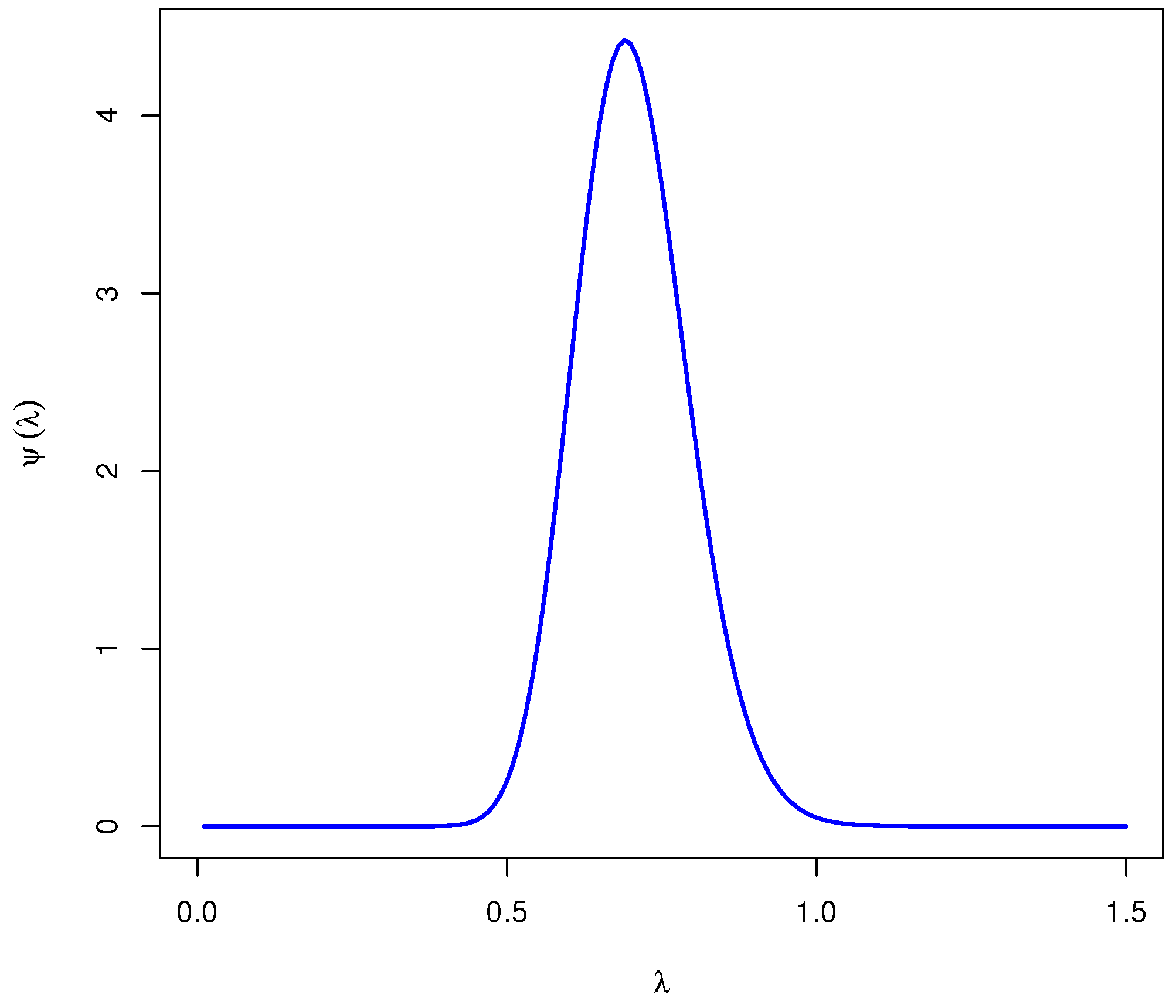
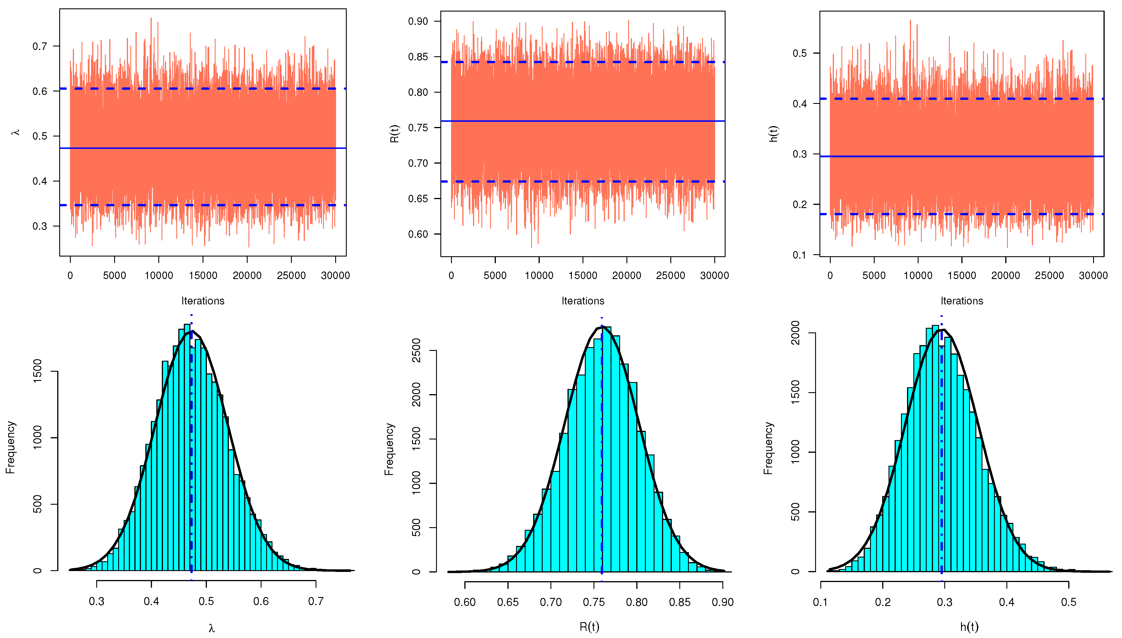
18) and then to obtain the Bayesian estimates as well as the corresponding HPD credible intervals. An important issue when using the M–H procedure is to select the proposal distribution of the parameter λ . A simple way is to plot the full conditional distribution in (18). Figure 1 shows that the distribution in (18) behaves similarly to the normal distribution. Therefore, to generate samples utilizing M–H procedure and calculate the Bayesian estimates of λ , RF and HRF and the associated HPD credible intervals, the following steps should be completed:
Step 1.
Set the start value for the parameter λ , say λ ( 0 ) = λ ^ .
Step 2.
Put j = 1 .
Step 3.
Generate λ from the full conditional distribution in (18) from the normal distribution N ( λ ( j 1 ) , v a r ( λ ( j 1 ) ) ) .
Step 4.
Calculate the ratio:
p ( λ ( j 1 ) | λ ) = min 1 , ψ ( λ ) ψ ( λ ( j 1 ) ) .
Step 5.
Generate w, where w U ( 0 , 1 ) .
Step 6.
If w p ( λ ( j 1 ) | λ ) , set λ ( j ) = λ , otherwise, set λ ( j ) = λ ( j 1 ) .
Step 7.
Based on a distinct value t, obtain R ( j ) ( t ) and h ( j ) ( t ) as
R ( j ) ( t ) = 1 + λ ( j ) t 1 + λ ( j ) 2 e λ ( j ) t
and
h ( j ) ( t ) = λ ( j ) 2 λ ( j ) + t + 2 1 + λ ( j ) 2 + λ ( j ) t .
Step 8.
Put j = j + 1 .
Step 9.
Redo Steps 3–8 H times to bring
λ ( 1 ) , R ( 1 ) ( t ) , h ( 1 ) ( t ) , , λ ( H ) , R ( H ) ( t ) , h ( H ) ( t ) .
Step 10.
Calculate the Bayesian estimates of λ , R ( t ) and h ( t ) employing the SEL function, after a burn-in period M, as
λ ˜ = 1 H M j = M + 1 H λ ( j ) , R ˜ ( t ) = 1 H M j = M + 1 H R ( j ) ( t ) and h ˜ ( t ) = 1 H M j = M + 1 H h ( j ) ( t ) .
Step 11.
To acquire the HPD credible intervals of λ , RF, and HRF: First, sort the generated samples of λ ( j ) , R ( j ) ( t ) and h ( j ) ( t ) after burn-in period as λ ( M + 1 ) , λ ( M + 2 ) , , λ ( H ) , R ( M + 1 ) ( t ) , R ( M + 2 ) ( t ) , , R ( H ) ( t ) and h ( M + 1 ) ( t ) , h ( M + 2 ) ( t ) , , h ( H ) ( t ) , respectively. Employing the procedure suggested by Chen and Shao [19], the 100 ( 1 α ) % two-sided HPD credible interval for the unknown parameter λ is given by
λ j * , λ j * + 1 α H M ,
where j * = M + 1 , M + 2 , , H is selected such that
λ j * + [ 1 α H M ] λ j * = min 1 j α ( H M ) ( λ ( j + [ 1 α H M ] ) λ ( j ) ) .
The largest integer less than or equal to x is denoted by [ x ] . Then, the HPD credible interval of x with the smallest length is that interval. The HPD credible intervals of RF and HRF can be easily computed using the same approach.

4. Monte Carlo Simulation

To evaluate the behavior of the proposed estimators of the unknown parameters λ , R ( t ) , and h ( t ) obtained in the proceeding sections, based on two different true values of λ as XL ( λ ) = XL ( 0.5 ) and XL ( 1.5 ) , some Monte Carlo simulations are conducted. At given time t = 0.1 , the true value of the reliability characteristics R ( t ) and h ( t ) are 0.972 and 0.283 for XL ( 0.5 ) as well as 0.881 and 1.266 for XL ( 1.5 ) , respectively. Using various combinations of n, m, R, and T, a 1000 adaptive Type-II progressively hybrid censored samples are generated. Using various choices of n (total sample size), ( m / n ) 100 % (failure information percentage (FIP)) and T (threshold time point) such as: n (=40, 80), m (=30, 60, 90)% and T (=1, 2), the simulation study is performed. Once the observed number of failed subjects achieves (or exceeds) a certain value m, the experiment is stopped.
In addition, to assess the performance of removal patterns R i , i = 1 , 2 , , m , various progressive censoring schemes (PCSs) are also taken into account as
PCS-1 : R 1 = n m , R i = 0 for i 1 , PCS-2 : R m 2 = n m , R i = 0 for i m / 2 , PCS-3 : R m = n m , R i = 0 for i m .
To simulate adaptive Type-II progressively hybrid censored samples of size m from a given sample of size n with given progressive Type-II censoring scheme R i , i = 1 , 2 , , m , perform the following procedure:
Step 1.
Generate an ordinary Type-II progressive censored sample ( X i , R i ) , i = 1 , 2 , , m , as discussed in Balakrishnan and Cramer [20] as
(i)
Generate m independent observations as y 1 , y 2 , , y m .
(ii)
Set υ i = y i i + j = m i + 1 m R j 1 , for i = 1 , 2 , , m .
(iii)
Set u i = 1 υ m υ m 1 υ m i + 1 for i = 1 , 2 , , m . Hence, u i , i = 1 , 2 , , m is a simulated sample of size m from the uniform U ( 0 , 1 ) distribution.
(iv)
Set X i = F 1 ( u i ; λ ) , i = 1 , 2 , , m , the Type-II progressive censored sample from XL ( λ ) is generated.
Step 2.
Obtain d-th failure and discard X i for i = d + 2 , , m .
Step 3.
Obtain order statistics X d + 2 , , X m from a truncated distribution f x / 1 F x d + 1 with sample size n d j = 1 d R j 1 .
To assess the performance of the gamma conjugate priors on the Bayesian estimates, by considering two information criteria for selecting the hyperparameter values called prior mean and prior variance, two sets of the hyperparameters ( a , b ) are used, namely:
  • Prior-I (say P1):(1.5, 3) and Prior-II (say P2):(2.5, 5) when XL ( 0.5 ) .
  • Prior-I (say P1):(4.5, 3) and Prior-II (say P2):(7.5, 5) when XL ( 1.5 ) .
Using the MCMC algorithm described in Section 3, 12,000 MCMC samples are generated and then the first 2,000 MCMC variates are discarded as burn-in. After that, the Bayes estimates of λ , R ( t ) , and h ( t ) utilizing the SEL function and associated 95% HPD credible intervals are computed based on the remaining 10,000 MCMC samples. However, based on each setting, both frequentist/Bayes point estimates as well as the asymptotic/HPD credible interval estimates of λ , R ( t ) , and h ( t ) are obtained. The average estimates of λ , R ( t ) , and h ( t ) (say ω ) based on any method are obtained as
ω ^ η ¯ = 1 D i = 1 D ω ^ η ( i ) , η = 1 , 2 , 3 ,
where D is the number of generated sequence data, ω ^ ( i ) is the calculated estimate of ω at the j-th simulated sample, ω 1 = λ , ω 2 = R ( t ) and ω 3 = h ( t ) .
Further, the comparison between the point estimates of ω is made based on their root mean squared errors (RMSEs) and mean relative absolute biases (MRABs) as
RMSE ( ω ^ η ) = 1 D i = 1 D ω ^ η ( i ) ω η 2 , η = 1 , 2 , 3
and
MRAB ( ω ^ η ) = 1 D i = 1 D 1 ω η ω ^ η ( i ) ω η , η = 1 , 2 , 3 ,
respectively. Furthermore, the comparison between interval estimates is made using their average confidence lengths (ACLs) and coverage percentages (CPs) given, respectively, by
ACL ( 1 α ) % ( ω ) = 1 D i = 1 D U ω ^ ( i ) L ω ^ ( i ) , η = 1 , 2 , 3 ,
and
CP ( 1 α ) % ( ω ) = 1 D i = 1 D 1 L ω ^ ( i ) ; U ω ^ ( i ) ω , η = 1 , 2 , 3 ,
where 1 ( · ) is the indicator function and L ( · ) and U ( · ) denote the lower and upper bounds of the interval estimate.
Using three useful packages programmed in R 4.1.2 software, namely, the ‘coda’ (by Plummer et al. [21]), ‘maxLik’ (by Henningsen and Toomet [22]), and ‘GoFKernel’ (by Pavia [23]) packages, all numerical evaluations were implemented. Recently, these packages were also recommended by Elshahhat and Nassar [24] and Elshahhat and Elemary [25]. The R 
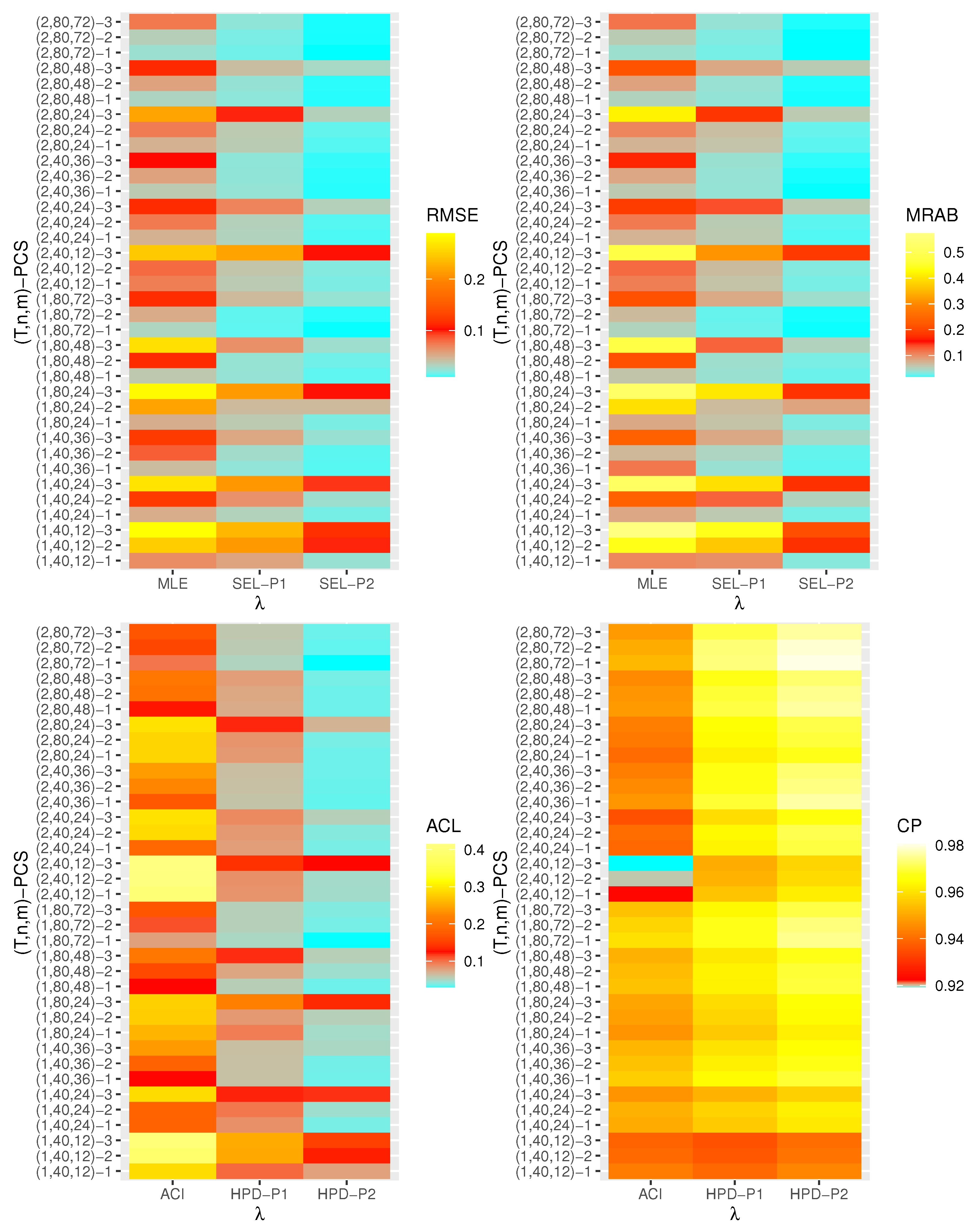
codes that support the findings of this study are available from the corresponding author upon reasonable request. All simulation results of λ , R ( t ) , and h ( t ) are displayed with heatmap plots in Figure 2, Figure 3, Figure 4, Figure 5, Figure 6 and Figure 7, respectively, while all numerical results are provided in the 
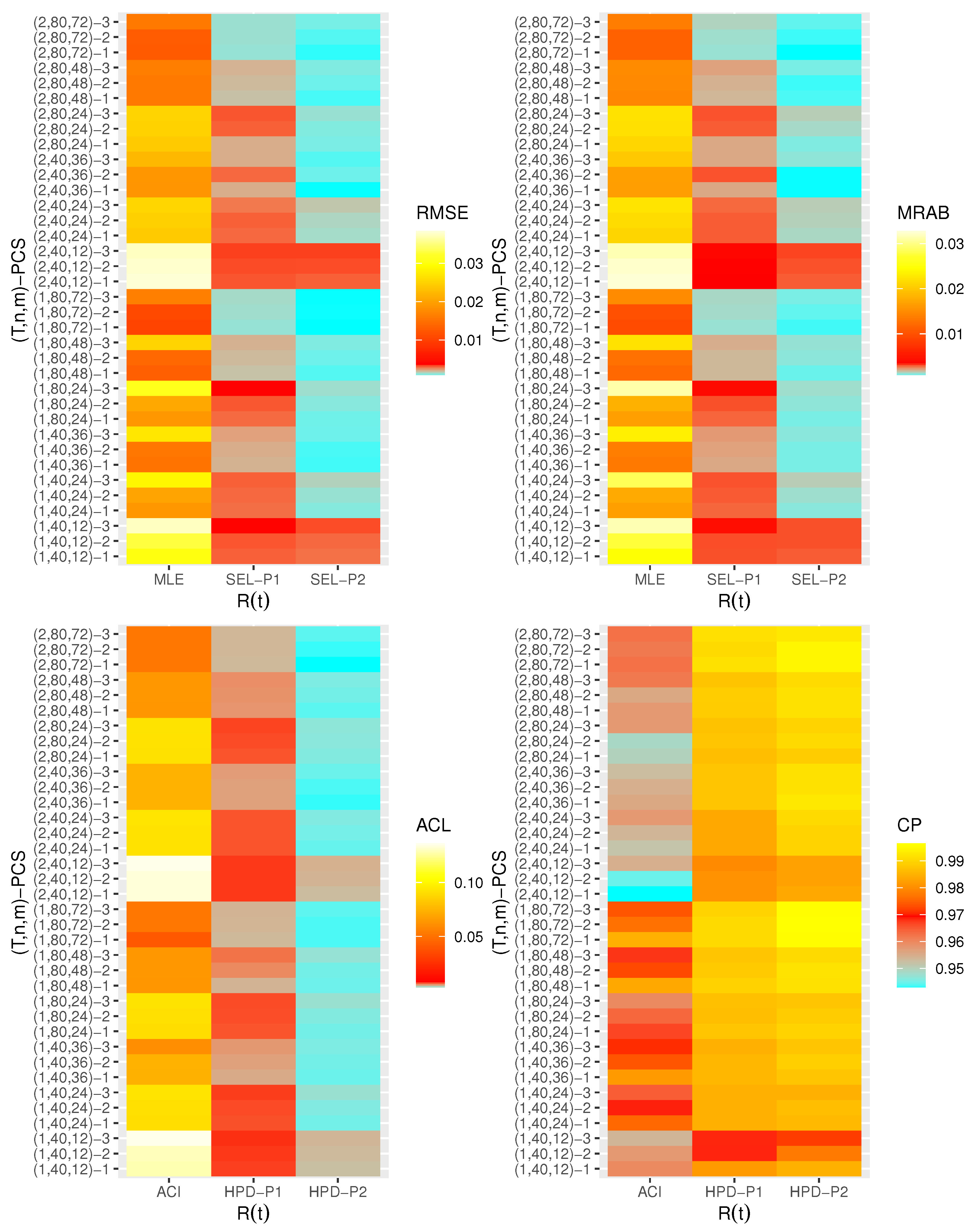
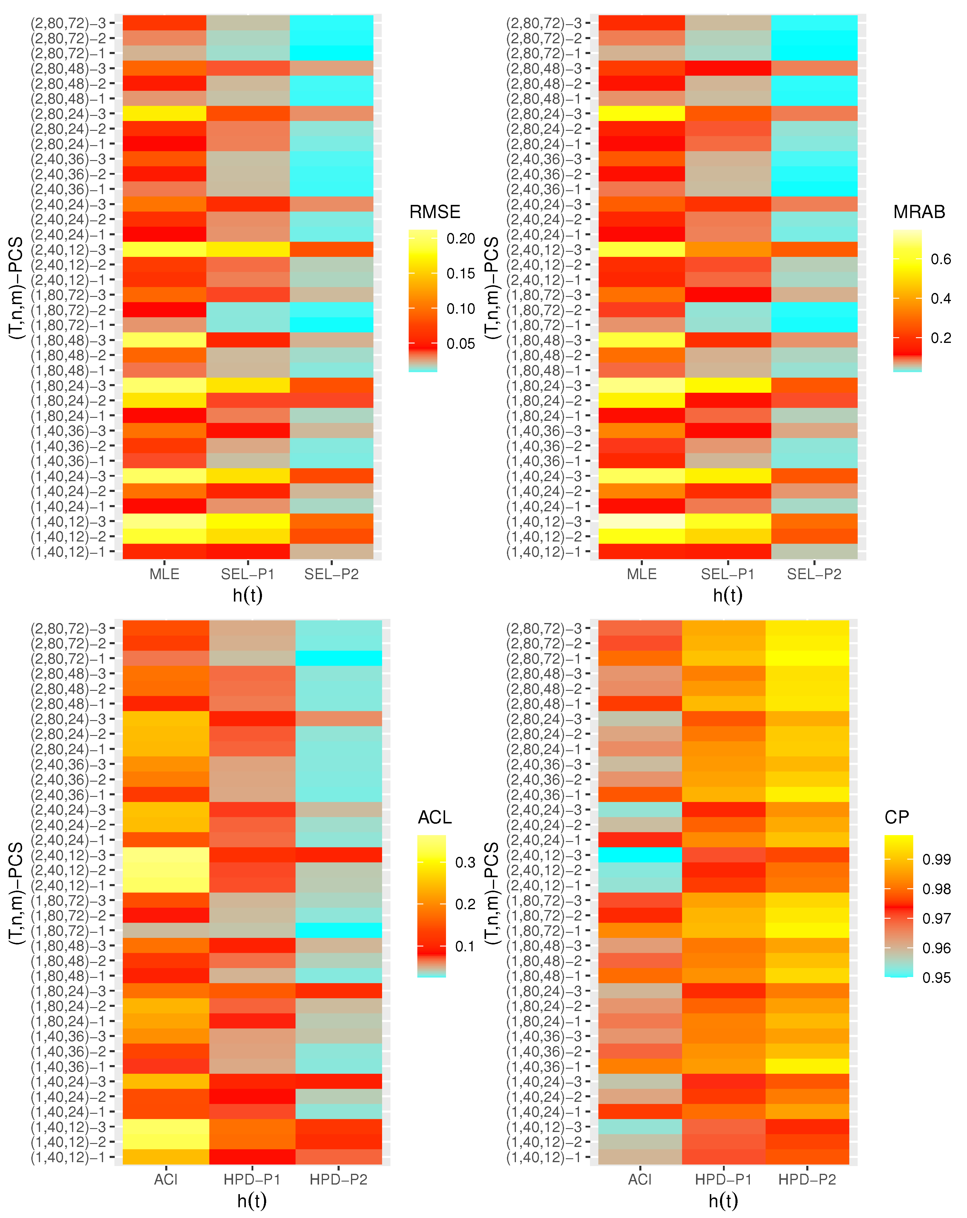
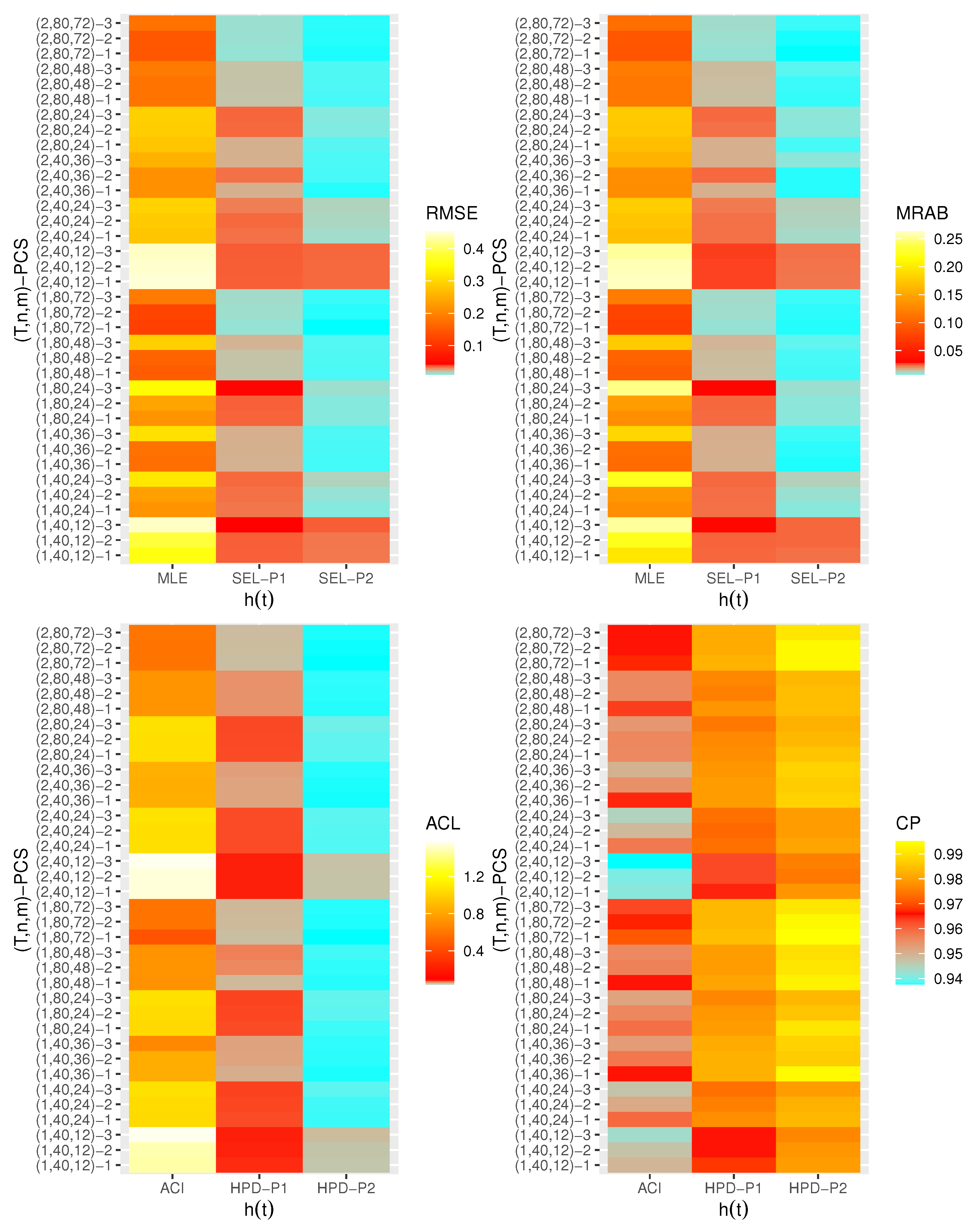
Supplementary File. In each heatmap plot, ‘ x - lab ’ displays the proposed estimation methods, while ‘ y - lab ’ represents the different choices of ( T , n , m ) -PCS. For designation, based on P1, for example, we have used the notation “SEL-P1” for the Bayes estimates from the SEL function and “HPD-P1” denotes to HPD credible intervals, respectively. In each heatmap, the colors vary from blue to yellow through red color. For example, in the case of the RMSE of λ in Figure 2, when the color tends to be blue, it indicates that the RMSE has a small value, while the yellow color refers to a high value of the RMSE. A moderate value for the RMSE is presented in red color. From Figure 2, Figure 3, Figure 4, Figure 5, Figure 6 and Figure 7, the following conclusions can be drawn:
  • Generally, the proposed estimates of the unknown parameters λ , R ( t ) , and h ( t ) behave well in terms of lowest RMSE, MRAB, and ACL values, as well as the highest CP values;
  • As n(or m) increases, all estimates of λ , R ( t ) , and h ( t ) perform better. A similar result is found in the case of the total number of removal patterns, as R i , i = 1 , 2 , , m , decreases;
  • Comparing PCSs 1, 2 and 3, we can observe that the RMSEs, MRABs, ACLs, and CPs of all unknown parameters are critically good based on PCS-1 (when the live items n m are removed at the first X ( 1 ) stage) compared to others. Since the expected duration of the life test experiment based on the first stage is greater than any other, the data collected under PCS-1 provided more information about the unknown parameters λ , R ( t ) , and h ( t ) than those obtained based on any others;
  • Comparing the gamma priors P1 and P2 on the Bayesian analysis, since the variance of P2 is less than the variance of P1, it can be seen that the Bayesian point/interval estimators of all unknown parameters from P2 perform more satisfactorily than those obtained from P1 in terms of the lowest RMSE, MRAB, and ACL values and largest CP values;
  • As T increases, the RMSEs and MRABs of all estimates of all unknown parameters for XL ( 0.5 ) decrease, while there is an increase for XL ( 1.5 ) ;
  • As T increases, the ACLs of all ACIs of all unknown parameters increase for both XL ( 0.5 ) and XL ( 1.5 ) , whereas the associated CPs decrease.
  • As T increases, the ACLs of all HPD credible interval estimates of all unknown parameters decrease for XL ( 0.5 ) and increase for XL ( 1.5 ) . The opposite behavior is also observed in case of the CPs for all HPD credible interval estimates of λ , R ( t ) , and h ( t ) ;
  • As λ increases, the RMSEs and MRABs of the MLEs of λ , R ( t ) , and h ( t ) increase, while those based on the MCMC of λ decrease and increase for R ( t ) and h ( t ) in most cases;
  • As λ increases, the associated ACLs of the ACIs of λ , R ( t ) , and h ( t ) become wider, while those based on the HPD credible interval estimates of λ decrease and increase for R ( t ) and h ( t ) in most cases. Additionally, as λ increases, the opposite behavior is noted in the case of CPs for ACI/HPD credible interval estimates of λ , R ( t ) , and h ( t ) ;
  • To sum up, the Bayesian paradigm utilizing the M–H algorithm is advised to estimate the scale parameter λ and the reliability indices RF and HRF of the XL distribution in the presence of the adaptive Type-II progressively hybrid censored scheme.

5. Real-Life Applications

The principal aim of this section is to demonstrate the usefulness of the proposed estimation methods and to show how the proposed estimators can be used in practice. Therefore, in this section, we investigate the analysis of two real data sets from the chemical engineering field.

5.1. Sodium Sulfur

The first application is to analyze one real data set that represents the lifetimes (in cycles) of sodium sulfur for twenty batteries. This data set was given by Ansell and Ansell [26] and reanalyzed by Phillips [27]. The lifetimes of sodium sulfur batteries (SSB) are: 76, 82, 210, 315, 385, 412, 491, 504, 522, 646+, 678, 775, 884, 1131, 1446, 1824, 1827, 2248, 2385, 3077. Note that lifetime observation with ‘+’ is right censored data. For computational convenience, each failure time point in the original SSB data set is divided by one thousand.
First, in addition to the gamma G ( α , λ ) and Weibull W ( α , λ ) distributions, the XL distribution is compared with other well-known competing distributions, namely: exponential E ( λ ) , Lindley L ( λ ) , and Xgamma X G ( λ ) proposed by Sen et al. [28]. To validate the proposed models, the Kolmogorov–Smirnov (KS) distance with its p-value is considered. Moreover, several measures of goodness of fit are also used namely: Akaike (A), Bayesian (B), consistent Akaike (CA) and Hannan–Quinn (HQ) information criteria. Clearly, the best lifetime model corresponds to the lowest value of KS distance, A, B, CA, and HQ criteria and largest p-value. The values of MLEs of the model parameters with their standard errors (SEs) in parentheses as well as the goodness-of-fit measures based on the SSB data set are computed and reported in Table 1. In this application, our calculations obtained here were developed based on only those observations which were completely observed and we left out those observations which were still running. Table 1 shows that the XLindley fits the SSB data quite well. It is also evident that XL distribution has the lowest values of A, CA, B, HQ, and KS goodness criteria, as well as the highest p-value. Thus, we can conclude that the XL distribution provides a better fit than all fitted competitive models based on the given SSB data set. For further appropriate clarification, Figure 8a presents the histogram of the SSB data and the fitted PDFs, while Figure 8b shows the empirical and fitted RFs. We also include the quantile–quantile (QQ) plots of all competitive distributions, as displayed in Figure 9. It is clear from these figures that the graphical representations support the same conclusion based on numerical results.
Using the complete SSB data set, three different artificial adaptive Type-II progressively hybrid censored samples (with m = 10 ) based on different PCSs are generated and reported in Table 2. For instance, the censoring scheme R = ( 2 , 1 , 1 , 1 , 2 ) is used as R = ( 2 , 1 * 3 , 2 ) . Via the M–H algorithm sampler, from 40,000 MCMC samples with 10,000 burn-in, the Bayes MCMC estimates of λ , R ( t ) , and h ( t ) (at time t = 1 ) with their SEs are developed using noninformative prior.
Furthermore, the two-sided 95% ACI/HPD credible interval estimates with their interval lengths (ILs) are calculated. The classical estimate of λ is chosen as the initial guess in order to run the MCMC algorithm. Based on the data in Table 2, all estimates of λ , R ( t ) , and h ( t ) are obtained and listed in Table 3. In Table 3, the SEs of point estimates as well as the ILs of interval estimates are tabulated in the second row corresponding to each unknown parameter. It is evident from Table 3 that the point estimates of λ , R ( t ) , and h ( t ) obtained by likelihood/Bayesian methods, as well as their interval estimates obtained by asymptotic/credible intervals, are similar.
To evaluate the convergence of MCMC procedure, using sample 1 information as an example, we trace plots of MCMC outputs of λ , R ( t ) , and h ( t ) with their sample mean (horizontal soled line (—)) and two bounds of 95% HPD credible intervals (horizontal dashed lines (- - -)) are shown in Figure 10. Additionally, using a Gaussian kernel based on the sample 1 information, the histograms of the simulated MCMC estimates of λ , R ( t ) , and h ( t ) with their sample mean (vertical dash-dotted line (:)) are also plotted in Figure 10. It shows that the MCMC technique converges very well and that the simulated MCMC variates of all unknown parameters are fairly symmetrical. Moreover, a comparison of the estimated HRFs based on the generated samples 1, 2, and 3 from the SSB data is plotted in Figure 11. It indicates that the estimated HRFs are clearly increasing in both maximum likelihood and Bayes methods.

5.2. Vinyl Chloride

Vinyl chloride is a colorless gas that burns easily and is a known human carcinogen. It must be produced industrially for use in commercial products, including pipes, wire and cable coatings, and packaging materials. Therefore, exposure to this gas should be avoided as much as possible and its levels should be kept as low as technically possible. This subsection presents analysis of 34 data points for vinyl chloride (in milligrams/liter) obtained from clean up-gradient monitoring wells as: 0.1, 0.1, 0.2, 0.2, 0.4, 0.4, 0.4, 0.5, 0.5, 0.5, 0.6, 0.6, 0.8, 0.9, 0.9, 1.0, 1.1, 1.2, 1.2, 1.3, 1.8, 2.0, 2.0, 2.3, 2.4, 2.5, 2.7, 2.9, 3.2, 4.0, 5.1, 5.3, 6.8, 8.0. This data set was reported by Bhaumik et al. [29] and recently analyzed by Elshahhat and Elemary [25]. Once again, using the same goodness-of-fit criteria discussed in Section 5.1, we fit the XL distribution to the complete vinyl chloride data set along with its competitors, namely, XG, E, L, G, and W distributions.
The fitted results of XL, XG, E, L, G, and W distributions based on vinyl chloride data are presented in Table 4. As a result, it can be seen that the XL distribution fits the vinyl chloride data quite satisfactorily, which implies that the XL distribution is the best model compared to other fitted models for the same real data. Moreover, the histogram of the vinyl chloride data and the fitted PDFs as well as the plot of fitted/empirical RFs of XL, XG, E, L, G, and W distributions are provided in Figure 12a,b. Further, from the vinyl chloride data, the QQ plots are depicted in Figure 13. Now, from the complete vinyl chloride data, three different adaptive Type-II progressively hybrid censored samples (using m = 14 and various choices of R) are generated and listed in Table 5.
From the data in Table 5, both frequentist and Bayes MCMC estimates with their SEs of the unknown parameters of λ , R ( t ) , and h ( t ) (at distinct time t = 1 are calculated and listed in Table 6. Moreover, two-sided 95% ACI/HPD interval estimates with their ILs are computed and are also presented in Table 6. It shows that the likelihood/Bayes (or ACI/HPD interval) estimates of λ , R ( t ) , and h ( t ) are very close to each other as expected.
For example, based on sample 1, trace and histogram plots of MCMC outputs of λ , R ( t ) , and h ( t ) are displayed in Figure 14. This indicates that the MCMC simulated variates of all unknown parameters converge well and behave symmetrically. Lastly, we can conclude that the proposed methodologies provide a good demonstration of the proposed XL lifetime model in the presence of chemical engineering data. Using the generated samples 1, 2, and 3 from vinyl chloride data, the corresponding estimated HRFs are displayed in Figure 15. This shows that the estimated HRFs based on both MLEs and MCMC estimates are increasingly behaving well.

6. Concluding Remarks

In this paper, we explored the estimation problems of the XLindley distribution using an adaptive progressive Type-II hybrid censored data. The maximum likelihood estimation method as a classical estimation method is considered for obtaining point estimators for the unknown parameter, reliability, and hazard rate functions. The associated approximate confidence intervals are also computed. Furthermore, the Bayesian approach is employed based on independent gamma priors and the Bayesian estimates are acquired using the squared-error loss function. The Bayesian estimators are obtained using the MCMC technique due to the complicated expression of the posterior distribution. Additionally, the highest posterior density credible intervals are computed. A simulation study was used to examine the performance of the various suggested estimators by considering different options for the sample sizes, the observed number of failures, and progressive censoring schemes. Two real data sets are examined to demonstrate the possible application of the suggested approaches. The results of the simulation study showed that the Bayesian technique yields point and interval estimates that are more accurate than those produced by the maximum likelihood approach. Moreover, the real data investigation revealed that the XLindley distribution yields more satisfactory results when compared with some other competitive models.

Supplementary Materials

The following information can be downloaded at: https://www.mdpi.com/article/10.3390/math10183355/s1, Table S1: The AEs (first-column), RMSEs (second-column) and MRABs (third-column) of λ when λ = 0.5; Table S2: The AEs (first-column), RMSEs (second-column) and MRABs (third-column) of λ when λ = 1.5; Table S3: The AEs (first-column), RMSEs (second-column) and MRABs (third-column) of R(t) when λ = 0.5; Table S4: The AEs (first-column), RMSEs (second-column) and MRABs (third-column) of R(t) when λ = 1.5; Table S5: The AEs (first-column), RMSEs (second-column) and MRABs (third-column) of h(t) when λ = 0.5; Table S6: The AEs (first-column), RMSEs (second-column) and MRABs (third-column) of h(t) when λ = 1.5; Table S7: The ACLs (first-column) and CPs (second-column) of ACI/HPD credible intervals of λ when λ = 0.5; Table S8: The ACLs (first-column) and CPs (second-column) of ACI/HPD credible intervals of λ when λ = 1.5; Table S9: The ACLs (first-column) and CPs (second-column) of ACI/HPD credible intervals of R(t) when λ = 0.5; Table S10: The ACLs (first-column) and CPs (second-column) of ACI/HPD credible intervals of R(t) when λ = 1.5; Table S11: The ACLs (first-column) and CPs (second-column) of ACI/HPD credible intervals of h(t) when λ = 0.5; Table S12: The ACLs (first-column) and CPs (second-column) of ACI/HPD credible intervals of h(t) when λ = 1.5.

Author Contributions

Methodology, R.A. and M.N.; Funding acquisition, R.A.; Software, A.E.; Supervision, A.E. and M.N.; Writing—original draft, M.N. and A.E.; Writing—review & editing, A.E. and R.A. All authors have read and agreed to the published version of the manuscript.

Funding

This research was funded by Princess Nourah bint Abdulrahman University Researchers Supporting Project number (PNURSP2022R50), Princess Nourah bint Abdulrahman University, Riyadh, Saudi Arabia.

Data Availability Statement

The authors confirm that the data supporting the findings of this study are available within the article.

Acknowledgments

The authors would like to express their thanks to the editor and the three anonymous referees for valuable comments and helpful observations. Princess Nourah bint Abdulrahman University Researchers Supporting Project number (PNURSP2022R50), Princess Nourah bint Abdulrahman University, Riyadh, Saudi Arabia.

Conflicts of Interest

The authors declare no conflict of interest.

References

  1. Kundu, D.; Joarder, A. Analysis of Type-II progressively hybrid censored data. Comput. Stat. Data Anal. 2006, 50, 2509–2528. [Google Scholar] [CrossRef]
  2. Ng, H.K.T.; Kundu, D.; Chan, P.S. Statistical analysis of exponential lifetimes under an adaptive Type-II progressive censoring scheme. Nav. Res. Logist. 2009, 56, 687–698. [Google Scholar] [CrossRef]
  3. Hemmati, F.; Khorram, E. On adaptive progressively Type-II censored competing risks data. Commun. Stat.-Simul. Comput. 2017, 46, 4671–4693. [Google Scholar] [CrossRef]
  4. Nassar, M.; Abo-Kasem, O.E. Estimation of the inverse Weibull parameters under adaptive type-II progressive hybrid censoring scheme. J. Comput. Appl. Math. 2017, 315, 228–239. [Google Scholar] [CrossRef]
  5. Ateya, S.F.; Mohammed, H.S. Statistical inferences based on an adaptive progressive type-II censoring from exponentiated exponential distribution. J. Egypt. Math. Soc. 2017, 25, 393–399. [Google Scholar] [CrossRef]
  6. Nassar, M.; Abo-Kasem, O.; Zhang, C.; Dey, S. Analysis of Weibull distribution under adaptive type-II progressive hybrid censoring scheme. J. Indian Soc. Probab. Stat. 2018, 19, 25–65. [Google Scholar] [CrossRef]
  7. Nassar, M.; Alotaibi, R.; Dey, S. Estimation Based on Adaptive Progressively Censored under Competing Risks Model with Engineering Applications. Math. Probl. Eng. 2022, 2022, 6731230. [Google Scholar] [CrossRef]
  8. Sobhi, M.M.A.; Soliman, A.A. Estimation for the exponentiated Weibull model with adaptive Type-II progressive censored schemes. Appl. Math. Model. 2016, 40, 1180–1192. [Google Scholar] [CrossRef]
  9. Panahi, H.; Moradi, N. Estimation of the inverted exponentiated Rayleigh distribution based on adaptive Type II progressive hybrid censored sample. J. Comput. Appl. Math. 2020, 364, 112345. [Google Scholar] [CrossRef]
  10. Chen, S.; Gui, W. Statistical analysis of a lifetime distribution with a bathtub-shaped failure rate function under adaptive progressive type-II censoring. Mathematics 2020, 8, 670. [Google Scholar] [CrossRef]
  11. Panahi, H.; Asadi, S. On adaptive progressive hybrid censored Burr type III distribution: Application to the nano droplet dispersion data. Qual. Technol. Quant. Manag. 2021, 18, 179–201. [Google Scholar] [CrossRef]
  12. Okasha, H.; Nassar, M.; Dobbah, S.A. E-Bayesian estimation of Burr Type XII model based on adaptive Type-II progressive hybrid censored data. AIMS Math. 2021, 6, 4173–4196. [Google Scholar] [CrossRef]
  13. Alotaibi, R.; Elshahhat, A.; Rezk, H.; Nassar, M. Inferences for Alpha Power Exponential Distribution Using Adaptive Progressively Type-II Hybrid Censored Data with Applications. Symmetry 2022, 14, 651. [Google Scholar] [CrossRef]
  14. Lindley, D.V. Fiducial distributions and Bayes’ theorem. J. R. Stat. Soc. Ser. B 1958, 20, 102–107. [Google Scholar] [CrossRef]
  15. Chouia, S.; Zeghdoudi, H. The XLindley Distribution: Properties and Application. J. Stat. Theory Appl. 2021, 20, 318–327. [Google Scholar] [CrossRef]
  16. Greene, W.H. Econometric Analysis, 4th ed.; Prentice-Hall: New York, NY, USA, 2000. [Google Scholar]
  17. Ahmed, E.A. Bayesian estimation based on progressive Type-II censoring from two-parameter bathtub-shaped lifetime model: An Markov chain Monte Carlo approach. J. Appl. Stat. 2014, 41, 752–768. [Google Scholar] [CrossRef]
  18. Dey, S.; Wang, L.; Nassar, M. Inference on Nadarajah–Haghighi distribution with constant stress partially accelerated life tests under progressive type-II censoring. J. Appl. Stat. 2021, 49, 2891–2912. [Google Scholar] [CrossRef]
  19. Chen, M.H.; Shao, Q.M. Monte Carlo estimation of Bayesian credible and HPD intervals. J. Comput. Graph. Stat. 1999, 8, 69–92. [Google Scholar]
  20. Balakrishnan, N.; Cramer, E. The Art of Progressive Censoring; Springer, Birkhäuser: New York, NY, USA, 2014. [Google Scholar]
  21. Plummer, M.; Best, N.; Cowles, K.; Vines, K. CODA: Convergence diagnosis and output analysis for MCMC. R News 2006, 6, 7–11. [Google Scholar]
  22. Henningsen, A.; Toomet, O. maxLik: A package for maximum likelihood estimation in R. Comput. Stat. 2011, 26, 443–458. [Google Scholar] [CrossRef]
  23. Pavia, J.M. Testing goodness-of-fit with the kernel density estimator: GoFKernel. J. Stat. Softw. 2015, 66, 1–27. [Google Scholar] [CrossRef]
  24. Elshahhat, A.; Nassar, M. Bayesian survival analysis for adaptive Type-II progressive hybrid censored Hjorth data. Comput. Stat. 2021, 36, 1965–1990. [Google Scholar] [CrossRef]
  25. Elshahhat, A.; Elemary, B.R. Analysis for Xgamma Parameters of Life under Type-II Adaptive Progressively Hybrid Censoring with Applications in Engineering and Chemistry. Symmetry 2021, 13, 2112. [Google Scholar] [CrossRef]
  26. Ansell, R.O.; Ansell, J.I. Modelling the reliability of sodium sulphur cells. Reliab. Eng. 1987, 17, 127–137. [Google Scholar] [CrossRef]
  27. Phillips, M.J. Statistical Methods for Reliability Data Analysis. In Handbook of Reliability Engineering; Springer: London, UK, 2003. [Google Scholar]
  28. Sen, S.; Maiti, S.S.; Chandra, N. The xgamma distribution: Statistical properties and application. J. Mod. Appl. Stat. Methods. 2016, 15, 774–788. [Google Scholar] [CrossRef]
  29. Bhaumik, D.K.; Kapur, K.; Gibbons, R.D. Testing parameters of a gamma distribution for small samples. Technometrics 2009, 51, 326–334. [Google Scholar] [CrossRef]
Figure 1. The full conditional distributions of λ .
Mathematics 10 03355 g001
Figure 2. The heatmaps for the estimation results of λ when λ = 0.5 .
Mathematics 10 03355 g002
Figure 3. The heatmaps for the estimation results of λ when λ = 1.5 .
Mathematics 10 03355 g003
Figure 4. The heatmaps for the estimation results of R ( t ) when λ = 0.5 .
Mathematics 10 03355 g004
Figure 5. The heatmaps for the estimation results of R ( t ) when λ = 1.5 .
Mathematics 10 03355 g005
Figure 6. The heatmaps for the estimation results of h ( t ) when λ = 0.5 .
Mathematics 10 03355 g006
Figure 7. The heatmaps for the estimation results of h ( t ) when λ = 1.5 .
Mathematics 10 03355 g007
Figure 8. Fitted XL and competing models from SSB data. (a) PDFs. (b) RFs.
Mathematics 10 03355 g008
Figure 9. The QQ plots of the XL and competing models from SSB data.
Mathematics 10 03355 g009
Figure 10. Trace plots (top-panel) and Histograms (bottom-panel) of λ , R ( t ) , and h ( t ) from SSB data.
Mathematics 10 03355 g010
Figure 11. Estimated hazard rate plots from the SSB data.
Mathematics 10 03355 g011
Figure 12. Fitted XL and competing models from vinyl chloride data. (a) PDFs. (b) RFs.
Mathematics 10 03355 g012
Figure 13. The QQ plots of the XL and competing models from vinyl chloride data.
Mathematics 10 03355 g013
Figure 14. Trace plots (top panel) and histograms (bottom panel) of λ , R ( t ) , and h ( t ) from vinyl chloride data.
Mathematics 10 03355 g014
Figure 15. Estimated hazard rate plots from the vinyl chloride data.
Mathematics 10 03355 g015
Table 1. Summary fit for the SSB data.
ModelMLE(SE)ACABHQKS
θ λ Distancep-Value
XL-1.1897(0.2230)40.327240.565541.267640.48700.10090.979
XG-1.7176(0.2910)40.334240.569541.278640.49400.11270.947
E-0.9859(0.2262)40.540140.775441.484640.70000.10910.959
L-1.4191(0.2466)41.327041.549242.322741.52130.10150.976
G1.1697(0.2119)1.0749(0.2228)41.820642.570643.709542.14030.12450.896
W1.2970(0.3788)1.2787(0.4537)41.800542.550543.689442.12020.11910.921
Table 2. Different generated samples from SSB data set.
Sample T ( d ) R R m * Censored Data
14(10) ( 9 , 0 * 9 ) 00.076, 0.775, 0.884, 1.131, 1.446, 1.824, 1.827, 2.248, 2.385, 3.077
20.7(5) ( 0 * 4 , 5 , 4 , 0 * 4 ) 40.076, 0.082, 0.210, 0.315, 0.385, 0.775, 0.884, 1.131, 1.446, 1.824
30.4(5) ( 0 * 9 , 9 ) 90.076, 0.082, 0.210, 0.315, 0.385, 0.412, 0.491, 0.504, 0.522, 0.678
Table 3. The point and interval estimates of λ , R ( t ) , and h ( t ) from SSB data.
SampleParameterMLEMCMCACIHPD
1 λ 0.79760.6233(0.4132,1.1820)(0.4033,0.8636)
0.19610.00070.76880.4603
R ( 1 ) 0.56160.6654(0.3457,0.7775)(0.5265,0.8049)
0.11010.00050.43180.2785
h ( 1 ) 0.59960.4340(0.3691,0.8301)(0.2246,0.6556)
0.11760.00060.46100.4310
2 λ 0.82610.6486(0.4388,1.2133)(0.4190,0.8862)
0.19760.00070.77460.4672
R ( 1 ) 0.54620.6502(0.3347,0.7578)(0.5085,0.7878)
0.10790.00040.42310.2793
h ( 1 ) 0.62750.4577(0.3845,0.8706)(0.2467,0.6868)
0.12400.00070.48610.4401
3 λ 1.24910.8647(0.6276,1.8706)(0.5382,1.1899)
0.31710.00101.24300.6517
R ( 1 ) 0.35760.5318(0.1353,0.5798)(0.3710,0.7054)
0.11340.00050.44440.3344
h ( 1 ) 1.05110.6673(0.3979,1.7043)(0.3529,0.9911)
0.33330.00101.30650.6382
Table 4. Summary fit for the vinyl chloride data.
ModelMLE(SE)ACABHQKS
θ λ Distancep-Value
XL-0.5321(0.0913)112.9052113.0302114.4316113.42570.08900.9507
XG-1.0313(0.1235)114.9701115.0951116.4965115.49060.13840.5330
E-0.7145(0.0944)113.4008113.5258114.9271113.92130.10810.8221
L-0.8238(0.1054)114.6073114.7323116.1336115.12780.13270.5878
G1.0627(0.2281)0.5654(0.1536)114.8263115.2134117.8790115.86740.09730.9042
W1.0121(0.1328)1.8855(0.3377)114.8996115.2867117.9523115.94070.09160.9376
Table 5. Different generated samples from vinyl chloride data.
Sample T ( d ) R R m * Censored Data
10.50(1) ( 10 , 10 , 0 * 12 ) 100.1, 0.6, 0.8, 0.9, 0.9, 1.0, 1.1, 1.2, 1.2, 1.3, 1.8, 2.0, 2.0, 2.3
21.15(7) ( 0 * 6 , 10 , 10 , 0 * 6 ) 00.1, 0.1, 0.2, 0.2, 0.4, 0.4, 0.4, 1.2, 3.2, 4.0, 5.1, 5.3, 6.8, 8.0
32.2(13) ( 0 * 12 , 10 , 10 ) 100.1, 0.1, 0.2, 0.2, 0.4, 0.4, 0.4, 0.5, 0.5, 0.5, 0.6, 0.6, 0.8, 2.3
Table 6. The point and interval estimates of λ , R ( t ) , and h ( t ) from vinyl chloride data.
SampleParameterMLEMCMCACIHPD
1 λ 0.52260.4730(0.3274,0.7178)(0.3464,0.6055)
0.09960.00040.39040.2591
R ( 1 ) 0.72670.7593(0.5848,0.8685)(0.6740,0.8424)
0.07240.00020.28370.1684
h ( 1 ) 0.33860.2951(0.2725,0.4047)(0.1807,0.4094)
0.03370.00030.13220.2287
2 λ 0.52120.4698(0.3192,0.7232)(0.3399,0.6063)
0.13010.00040.40400.2664
R ( 1 ) 0.72750.7614(0.5806,0.8745)(0.6735,0.8466)
0.07500.00030.29390.1731
h ( 1 ) 0.33740.2923(0.2692,0.4055)(0.1746,0.4093)
0.03480.00030.13630.2347
3 λ 0.56660.5135(0.3577,0.7754)(0.3764,0.6473)
0.10660.00040.41770.2709
R ( 1 ) 0.69850.7331(0.5526,0.8444)(0.6456,0.8197)
0.07440.00030.29170.1741
h ( 1 ) 0.37900.3313(0.2998,0.4581)(0.2106,0.4546)
0.04040.00040.15830.2440
Publisher’s Note: MDPI stays neutral with regard to jurisdictional claims in published maps and institutional affiliations.

