Hermite-Hadamard-Type Integral Inequalities for Convex Functions and Their Applications

Abstract

In this paper, we establish new generalizations of the Hermite-Hadamard-type inequalities. These inequalities are formulated in terms of modules of certain powers of proper functions. Generalizations for convex functions are also considered. As applications, some new inequalities for the digamma function in terms of the trigamma function and some inequalities involving special means of real numbers are given. The results also include estimates via arithmetic, geometric and logarithmic means. The examples are derived in order to demonstrate that some of our results in this paper are more exact than the existing ones and some improve several known results available in the literature. The constants in the derived inequalities are calculated; some of these constants are sharp. As a visual example, graphs of some technically important functions are included in the text.

1. Introduction

The Hermite-Hadamard-type inequalities are very important in many topics of mathematics and its applications, and its original version is defined in the following way [1,2]:

$$h\left(\frac{a+b}{2}\right)\leqq \frac{1}{b-a}{\int }_a^{b}h\left(x\right)dx\leqq \frac{h\left(a\right)+h\left(b\right)}{2},$$

(1)

where a convex function h is defined on the interval $I\subseteq \mathbb{R}\to \mathbb{R}$ for real numbers $a,b\in I(a < b)$.

The Hermite-Hadamard-type inequalities (1) are an important instrument in abstract and applied mathematical fields, such as mathematical analysis, function theory, optimization, control theory, the theory of special means and different variants of entropy problems, interpolations and approximations, numerical methods including numerical integration, information theory, probability and statistics. The results of this article may be applied to integral inequalities for fractional interval-valued functions and the corresponding differential equations and optimization problems. Integral inequalities of the Hermite-Hadamard type are also important in the transmutation theory for estimating different kinds of kernels for transmutational operators (see [3]). Thus, obviously, the results of this paper are matched with the topic of this Special Issue, “Analytical and Computational Methods in Differential Equations, Special Functions, Transmutations and Integral Transforms”.

A considerable amount of work on these types of inequalities are known and recently, new proofs, generalizations, refinements, computer and numerical applications and illustrations were developed. As a result, many authors have focused on the Hermite-Hadamard-type inequalities for various classes of convex functions and mappings (see, for instance, [1,2,4,5,6,7,8,9,10,11,12,13,14,15,16,17,18,19,20,21,22,23]; see also the references cited therein).

From among very recent important papers, let us mention [20] in its connections with inclusion theory, and fuzzy sets are studied with the use of an interval analysis. Namely, different kinds of convexity and non-convexity conditions lead to interesting classes of inequalities, including problems with inclusions. For studying fuzzy order relations, an idea of logarithmic convexity is vital and fruitful. In this way, various discrete forms of Hermite-Hadamard and Jensen and Schur inequalities are studied for fuzzy interval-valued functions based upon considerations for logarithmic convex settings. It leads to new ideas and novel approaches in fuzzy optimization problems and interval-valued functions and the corresponding mathematical modeling. Moreover, the connected notion of interval-valued preinvex functions is also exploited; as an example, in [21], it is applied to the Riemann–Liouville fractional integrals in fractional calculus.

Dragomir and Agarwal [7], among other important results, proved the following inequality connected with the right-hand side of the inequality (1):

Theorem 1.

If h is a differentiable function on an interval $[a,b],$ and $|h^{\prime }|$ is a convex function on $[a,b],$ then the following inequality holds true:

$$\left|\frac{h\left(a\right)+h\left(b\right)}{2}-\frac{1}{b-a}{\int }_a^{b}h\left(x\right)dx\right|\leqq \frac{b-a}{8}\left(|h^{\prime }\left(a\right)|+|h^{\prime }\left(b\right)|\right).$$

(2)

Kirmaci [12] proved the following result connected with the left part of the inequality (1).

Theorem 2.

Under assumptions of the above Theorem A, the following holds true:

$$\left|h\left(\frac{a+b}{2}\right)-\frac{1}{b-a}{\int }_a^{b}h\left(x\right)dx\right|\leqq \frac{b-a}{8}\left(|h^{\prime }\left(a\right)|+|h^{\prime }\left(b\right)|\right).$$

(3)

Other interesting results in this direction were proved in [23], with several refinements and extensions of the Hermite–Hadamard and Jensen inequalities in n variables.

In this paper, we establish some new Hermite-Hadamard-type inequalities for a class of functions with convex derivatives under some conditions. As consequences of our results, new inequalities involving the digamma and trigamma functions are obtained and some inequalities involving special means of real numbers are given. The analytical and numerical computation shows that the obtained results are better than the corresponding similar inequalities in (2) and (3).

2. New Hermite-Hadamard-Type Inequalities for Convex Functions

The notion of convexity is very important and basic in mathematics. For results on convex functions, we may mention references [1,2,24,25,26,27].

The following lemma is very useful to obtain the results of this paper. Its proof is based on an integration by parts. We, therefore, omit the details involved.

Lemma 1.

Let h be an absolutely continuous function on an interval $[a,b]$ and let its derivative $h^{\prime }\in L_1[a,b]$. Then the following result holds true:

$$\begin{array}{c}\frac{1}{3}\left[h\left(a\right)+h\left(\frac{a+b}{2}\right)+h\left(b\right)\right]-\frac{1}{b-a}{\int }_a^{b}h\left(x\right)dx\hfill \\ =(b-a)[{\int }_0^{\frac{1}{2}}\left(x-\frac{1}{3}\right)h^{\prime }\left(a+x(b-a)\right)dx\hfill \\ +{\int }_{\frac{1}{2}}^1(x-\frac{2}{3})h^{\prime }\left(a+x(b-a)\right)dx].\hfill \end{array}$$

(4)

Theorem 3.

Let h be an absolutely continuous function on an interval $[a,b]$ and let its derivative $h^{\prime }\in L_1[a,b]$. Suppose also that $|h^{\prime }{|}^q$ is convex on $[a,b]$ for some $q\geqq 1$. Then the following result holds true:

$$\begin{array}{cc}\hfill & |\frac{1}{3}\left[h\left(a\right)+h\left(\frac{a+b}{2}\right)+h\left(b\right)\right]-\frac{1}{b-a}{\int }_a^{b}h\left(x\right)dx|\leqq (b-a){\left(\frac{5}{72}\right)}^{1-\frac{1}{q}}\hfill \\ \hfill & ·\left\{{\left(\frac{111|h^{\prime }{\left(a\right)|}^q}{1944}+\frac{|h^{\prime }{\left(b\right)|}^q}{81}\right)}^{\frac{1}{q}}+{\left(\frac{|h^{\prime }{\left(a\right)|}^q}{81}+\frac{111|h^{\prime }{\left(b\right)|}^q}{1944}\right)}^{\frac{1}{q}}\right\}.\hfill \end{array}$$

(5)

Proof. 

From Lemma 1, we have

$$\begin{array}{cc}\hfill & |\frac{1}{3}\left[h\left(a\right)+h\left(\frac{a+b}{2}\right)+h\left(b\right)\right]-\frac{1}{b-a}{\int }_a^{b}h\left(x\right)dx|\hfill \\ \hfill & =(b-a)|{\int }_0^{\frac{1}{2}}\left(x-\frac{1}{3}\right)h^{\prime }\left(a+x(b-a)\right)dx\hfill \\ \hfill & +{\int }_{\frac{1}{2}}^1\left(x-\frac{2}{3}\right)h^{\prime }\left(a+x(b-a)\right)dx|\hfill \\ \hfill & \leqq (b-a)\{{\int }_0^{\frac{1}{2}}\left|x-\frac{1}{3}\right|\left|h^{\prime }\left(a+x(b-a)\right)\right|dx\hfill \\ \hfill & +{\int }_{\frac{1}{2}}^1\left|x-\frac{2}{3}\right|\left|h^{\prime }\left(a+x(b-a)\right)\right|dx\}.\hfill \end{array}$$

(6)

Firstly, we assume that $q=1$, and by using the fact that the function $|h^{\prime }|$ is convex on $[a,b]$, we derive the following inequality:

$$\begin{array}{cc}\hfill & {\int }_0^{\frac{1}{2}}\left|x-\frac{1}{3}\right|\left|h^{\prime }\left(a+x(b-a)\right)\right|dx+{\int }_{\frac{1}{2}}^1\left|x-\frac{2}{3}\right|\left|h^{\prime }\left(a+x(b-a)\right)\right|dx\hfill \\ \hfill & \leqq {\int }_0^{\frac{1}{2}}\left|x-\frac{1}{3}\right|\left[(1-x)\left|h^{\prime }\left(a\right)\right|+x\left|h^{\prime }\left(b\right)\right|\right]dx\hfill \\ \hfill & +{\int }_{\frac{1}{2}}^1\left|x-\frac{2}{3}\right|\left((1-x)\left|h^{\prime }\left(a\right)\right|+x\left|h^{\prime }\left(b\right)\right|\right)dx\hfill \\ \hfill & \leqq \left|h^{\prime }\left(a\right)\right|\left({\int }_0^{\frac{1}{2}}(1-x)\left|x-\frac{1}{3}\right|+{\int }_{\frac{1}{2}}^1(1-x)\left|x-\frac{2}{3}\right|dx\right)\hfill \\ \hfill & +\left|h^{\prime }\left(b\right)\right|\left({\int }_0^{\frac{1}{2}}x\left|x-\frac{1}{3}\right|+{\int }_{\frac{1}{2}}^{1}x\left|x-\frac{2}{3}\right|dx\right)\hfill \\ \hfill & =\frac{5\left(\left|h^{\prime }\left(a\right)\right|+\left|h^{\prime }\left(b\right)\right|\right)}{72}.\hfill \end{array}$$

(7)

Therefore, the desired inequality asserted by Theorem 3 in the case $q=1$ holds true.

Now, we suppose that $q>1.$ Further, we will use the Hölder integral inequality in the classical settings for $L_p-L_q$ functions; About this inequality, see, e.g., the monograph [2]. Thus, from the Hölder integral inequality (with $p=\frac{q}{q-1}$), we obtain

$$\begin{array}{cc}\hfill & {\int }_0^{\frac{1}{2}}\left|x-\frac{1}{3}\right|\left|h^{\prime }\left(a+x(b-a)\right)\right|dx\hfill \\ \hfill & ={\int }_0^{\frac{1}{2}}{\left|x-\frac{1}{3}\right|}^{1-\frac{1}{q}}\left({\left|x-\frac{1}{3}\right|}^{\frac{1}{q}}\left|h^{\prime }\left(a+x(b-a)\right)\right|\right)dx\hfill \\ \hfill & \leqq {\left({\int }_0^{\frac{1}{2}}\left|x-\frac{1}{3}\right|dx\right)}^{1-\frac{1}{q}}{\left({\int }_0^{\frac{1}{2}}\left|x-\frac{1}{3}\right|{\left|h^{\prime }\left(a+x(b-a)\right)\right|}^{q}dx\right)}^{\frac{1}{q}}\hfill \\ \hfill & \leqq {\left(\frac{5}{72}\right)}^{1-\frac{1}{q}}{\left(|h^{\prime }{\left(a\right)|}^q{\int }_0^{\frac{1}{2}}(1-x)\left|x-\frac{1}{3}\right|dx+{\left|h^{\prime }\left(b\right)\right|}^q{\int }_0^{\frac{1}{2}}x\left|x-\frac{1}{3}\right|dx\right)}^{\frac{1}{q}}\hfill \\ \hfill & \leqq {\left(\frac{5}{72}\right)}^{1-\frac{1}{q}}{\left(\frac{111|h^{\prime }{\left(a\right)|}^q}{1944}+\frac{|h^{\prime }{\left(b\right)|}^q}{81}\right)}^{\frac{1}{q}}.\hfill \end{array}$$

(8)

In the same way, we find that

$${\int }_{\frac{1}{2}}^1\left|x-\frac{2}{3}\right|\left|h^{\prime }\left(a+x(b-a)\right)\right|dx\leqq {\left(\frac{5}{72}\right)}^{1-\frac{1}{q}}{\left(\frac{|h^{\prime }{\left(a\right)|}^q}{81}+\frac{111|h^{\prime }{\left(b\right)|}^q}{1944}\right)}^{\frac{1}{q}}.$$

(9)

Keeping (6), (8) and (9) in mind, we obtain the result (5) asserted by Theorem 3. □

Theorem 4.

Let h be an absolutely continuous function on an interval $[a,b]$ and let its derivative $h^{\prime }\in L_1[a,b].$ Suppose also that $|h^{\prime }{|}^q$ is convex on $[a,b]$ for some $q>1$. Then the following result holds true:

$$\begin{array}{cc}\hfill & \left|\frac{1}{3}\left[h\left(a\right)+h\left(\frac{a+b}{2}\right)+h\left(b\right)\right]-\frac{1}{b-a}{\int }_a^{b}h\left(x\right)dx\right|\hfill \\ \hfill & \leqq \frac{b-a}{12}{\left(\frac{1+2^{p+1}}{3(p+1)}\right)}^{\frac{1}{p}}{\left[|h^{\prime }{\left(a\right)|}^q+{\left|h^{\prime }\left(b\right)\right|}^q\right]}^{\frac{1}{q}}\hfill \end{array}$$

(10)

with

$$\frac{1}{p}+\frac{1}{q}=1.$$

Proof. 

As the function $|h^{\prime }{|}^q$ is convex on $[a,b]$, we have

$${\int }_0^{\frac{1}{2}}{\left|h^{\prime }\left(a+x(b-a)\right)\right|}^{q}dx\leqq \frac{3{\left|h^{\prime }\left(a\right)\right|}^q+{\left|h^{\prime }\left(b\right)\right|}^q}{8},$$

and

$${\int }_{\frac{1}{2}}^1{\left|h^{\prime }\left(a+x(b-a)\right)\right|}^{q}dx\leqq \frac{{\left|h^{\prime }\left(a\right)\right|}^q+3{\left|h^{\prime }\left(b\right)\right|}^q}{8}.$$

Straightforward calculation yields

$${\int }_0^{\frac{1}{2}}|x-\frac{1}{3}{|}^{p}dx={\int }_{\frac{1}{2}}^1|x-\frac{2}{3}{|}^{p}dx=\frac{1+2^{p+1}}{6^{p+1}(p+1)}.$$

(11)

Thus, by applying the Hölder integral inequality, we obtain

$$\begin{array}{cc}\hfill & {\int }_0^{\frac{1}{2}}\left|x-\frac{1}{3}\right|·\left|h^{\prime }\left(a+x(b-a)\right)\right|dx\hfill \\ \hfill & \leqq {\left({\int }_0^{\frac{1}{2}}{\left|x-\frac{1}{3}\right|}^{p}dx\right)}^{\frac{1}{p}}{\left({\int }_0^{\frac{1}{2}}{\left|h^{\prime }\left(a+x(b-a)\right)\right|}^{q}dx\right)}^{\frac{1}{q}}\hfill \\ \hfill & \leqq {\left(\frac{1+2^{p+1}}{6^{p+1}(p+1)}\right)}^{\frac{1}{p}}{\left(\frac{3{\left|h^{\prime }\left(a\right)\right|}^q+{\left|h^{\prime }\left(b\right)\right|}^q}{8}\right)}^{\frac{1}{q}},\hfill \end{array}$$

(12)

and

$$\begin{array}{cc}\hfill & {\int }_{\frac{1}{2}}^1\left|x-\frac{2}{3}\right|·\left|h^{\prime }\left(a+x(b-a)\right)\right|dx\hfill \\ \hfill & \leqq {\left({\int }_{\frac{1}{2}}^1{\left|x-\frac{2}{3}\right|}^{p}dx\right)}^{\frac{1}{p}}{\left({\int }_0^{\frac{1}{2}}{\left|h^{\prime }\left(a+x(b-a)\right)\right|}^{q}dx\right)}^{\frac{1}{q}}\hfill \\ \hfill & \leqq {\left(\frac{1+2^{p+1}}{6^{p+1}(p+1)}\right)}^{\frac{1}{p}}{\left(\frac{{\left|h^{\prime }\left(a\right)\right|}^q+3{\left|h^{\prime }\left(b\right)\right|}^q}{8}\right)}^{\frac{1}{q}}.\hfill \end{array}$$

(13)

Finally, upon combining (6), (12) and (13) and making some elementary simplifications, the asserted result (10) follows. □

Next, for the sake of brevity, we define

$$\mathsf{\Xi }(a,b):=\frac{1}{3}\left[h\left(a\right)+h\left(b\right)+h\left(A(a,b)\right)\right]-\frac{1}{b-a}{\int }_a^{b}h\left(x\right)dx\ne 0$$

and

$$A(a,b):=\frac{a+b}{2}.$$

As usual, we denote by $A(a,b)$ an arithmetic mean of two non-negative numbers a and b.

Theorem 5.

Under the conditions of Theorem 3, the following Hermite-Hadamard-type inequality holds true:

$$\begin{array}{cc}\hfill & \left|h\left(\frac{a+b}{2}\right)-\frac{1}{b-a}{\int }_a^{b}h\left(x\right)dx\right|\leqq (b-a)\left|{\rho }_1(a,b)\right|{\left(\frac{5}{72}\right)}^{1-\frac{1}{q}}\hfill \\ \hfill & ·\left\{{\left(\frac{111|h^{\prime }{\left(a\right)|}^q}{1944}+\frac{|h^{\prime }{\left(b\right)|}^q}{81}\right)}^{\frac{1}{q}}+{\left(\frac{|h^{\prime }{\left(a\right)|}^q}{81}+\frac{111|h^{\prime }{\left(b\right)|}^q}{1944}\right)}^{\frac{1}{q}}\right\},\hfill \end{array}$$

(14)

where

$${\rho }_1(a,b):=1-2\frac{A\left(h\left(a\right),h\left(b\right)\right)-h\left(A(a,b)\right)}{3\mathsf{\Xi }(a,b)}.$$

Furthermore, the next result is true:

$$\left|h\left(\frac{a+b}{2}\right)-\frac{1}{b-a}{\int }_a^{b}h\left(x\right)dx\right|\leqq \frac{5(b-a)|{\rho }_1(a,b)|}{72}\left[\left|h^{\prime }\left(a\right)\right|+\left|h^{\prime }\left(b\right)\right|\right].$$

(15)

Proof. 

With the aid of the Formula (4), we obtain

$$\begin{array}{cc}\hfill & \left|h\left(\frac{a+b}{2}\right)-\frac{1}{b-a}{\int }_a^{b}h\left(x\right)dx\right|\hfill \\ \hfill & =(b-a)|{\int }_0^{\frac{1}{2}}(x-\frac{1}{3})h^{\prime }\left(a+x(b-a)\right)dx+{\int }_{\frac{1}{2}}^1(x-\frac{2}{3})h^{\prime }\left(a+x(b-a)\right)dx\hfill \\ \hfill & -\frac{2}{3}\left(\frac{A\left(h\left(a\right),h\left(b\right)\right)-h\left(A(a,b)\right)}{(b-a)}\right)|\hfill \\ \hfill & =(b-a)\left|{\int }_0^{\frac{1}{2}}(x-\frac{1}{3})h^{\prime }\left(a+x(b-a)\right)dx+{\int }_{\frac{1}{2}}^1(x-\frac{2}{3})h^{\prime }\left(a+x(b-a)\right)dx\right|\hfill \\ \hfill & ·\left|1-\frac{2}{3}\left(\frac{A\left(h\left(a\right),h\left(b\right)\right)-h\left(A(a,b)\right)}{\mathsf{\Xi }(a,b)}\right)\right|.\hfill \end{array}$$

(16)

Obviously, by repeating the same calculations as in the proof of Theorem 3 with the help of (16), we achieve the required result (14).

Finally, taking $q=1$ in (14) leads to the inequality (15). This completes the proof of Theorem 5. □

Remark 1.

We note that, if $|{\rho }_1| < \frac{9}{5},$ then the inequality (15) is better than the inequality (3). It means that the absolute positive constant at the right-hand side of the inequality (15) is smaller, and so better, than the right-hand side of the inequality (3). Consequently, under the above condition $|{\rho }_1| < \frac{9}{5},$ the inequality (15) is more exact than the inequality (3).

Now, we present some examples to illustrate cases that the right-hand side of inequality (15) is better than the right-hand side of inequality (3).

• Let us consider the function $h\left(x\right)=e^x$ and $[a,b]=[t,t+1],t\in \mathbb{R}.$ Then, we have

  $${\rho }_1=\frac{3+3\sqrt{e}-3e}{4+\sqrt{e}-2e}\approx -0.98362.$$
  Consequently, the inequality (15) is better than the inequality (3). It means that the positive constant on the right-hand side of the inequality (15) is smaller (better!) than the positive constant on the right-hand side of the inequality (3).
• Let us take $h\left(x\right)=\psi \left(x\right)$, where

  $$\psi \left(x\right):=\frac{{\mathsf{\Gamma }}^{\prime }\left(x\right)}{\mathsf{\Gamma }\left(x\right)}$$

  is the digamma function and $[a,b]=[t,t+2](t>0).$ It is known that the trigamma function ${\psi }^{\prime }\left(x\right)$ is convex on $(0,\infty ).$ Hence, by using the following identity:

  $$\psi (t+1)=\psi \left(t\right)+\frac{1}{t},$$

  (17)

  we have

  $$A\left(h\left(t\right),h(t+2)\right)-h\left(A(t,t+2)\right)=-\frac{1}{2t(t+1)}$$

  and

  $$\mathsf{\Xi }(t,t+2)=\psi \left(t\right)+\frac{2}{3t}+\frac{1}{3(t+1)}-\frac{1}{2}log(t^2+t).$$
  Therefore, we get

  $${\rho }_1(t,t+2)=1+\frac{2}{6t(t+1)\psi \left(t\right)-3t(t+1)log\left(t(t+1)\right)+6t+4}.$$
  Hence, we obtain

  $$F\left(t\right):=|{\rho }_1(t,t+2)| < \frac{9}{5}$$

  for all $t>0$ (see Figure 1 which verifies our claim). Consequently, for this case, the right-hand side of the inequality (15) is better than the right-hand side of the inequality (3).
• Next, we let $h\left(x\right)=\psi \left(x\right)$ and $[a,b]=[t,t+1](t>0)$. Hence, for this case, we have

  $$A\left(h\left(t\right),h(t+1)\right)-h\left(A(t,t+1)\right)=\psi \left(t\right)-\psi \left(t+\frac{1}{2}\right)+\frac{1}{2t},$$

  and

  $$\mathsf{\Xi }(t,t+1)=\frac{2}{3}\psi \left(t\right)+\frac{1}{3}\psi \left(t+\frac{1}{2}\right)-logt+\frac{1}{3t}.$$
  Hence, we obtain

  $${\rho }_1(t,t+1)=\frac{3t\psi (t+1/2)-3tlogt}{2t\psi \left(t\right)+t\psi (t+1/2)-3tlogt+1}.$$
  By Figure $,$ we see that

  $$G\left(t\right):=|{\rho }_1(t,t+1)| < \frac{9}{5},$$

  which implies that (15) improves (3).

Theorem 6.

Under the conditions of Theorem 4, it is asserted that

$$\begin{array}{cc}\hfill & \left|h\left(\frac{a+b}{2}\right)-\frac{1}{b-a}{\int }_a^{b}h\left(x\right)dx\right|\hfill \\ \hfill & \leqq \frac{(b-a)|{\rho }_1(a,b)|}{12}{\left(\frac{1+2^{p+1}}{3(p+1)}\right)}^{\frac{1}{p}}{\left[|h^{\prime }{\left(a\right)|}^q+{\left|h^{\prime }\left(b\right)\right|}^q\right]}^{\frac{1}{q}}\hfill \end{array}$$

(18)

for

$$\frac{1}{p}+\frac{1}{q}=1.$$

In particular, the following inequality holds true:

$$\begin{array}{cc}\hfill & \left|h\left(\frac{a+b}{2}\right)-\frac{1}{b-a}{\int }_a^{b}h\left(x\right)dx\right|\hfill \\ \hfill & \leqq \frac{(b-a)|{\rho }_1(a,b)|}{12}{\left[|h^{\prime }{\left(a\right)|}^2+{\left|h^{\prime }\left(b\right)\right|}^2\right]}^{\frac{1}{2}}.\hfill \end{array}$$

(19)

Proof. 

By using the same consequent steps as in Theorem 4 with the help of the Formula (16), we obtain the inequality (18) asserted by Theorem 6. We choose to omit the details involved. □

Remark 2.

Under the conditions of Theorem 6, we see that the left-hand side of the inequality (19) is better than the inequality (3) if $|{\rho }_1(a,b)| < \frac{3}{2}.$ It means that the absolute positive constant on the right-hand side of the inequality (19) is smaller, and so better, than the right-hand side of the inequality (3). Consequently, under the above condition $|{\rho }_1(a,b)| < \frac{3}{2},$ the inequality (19) is more exact than the inequality (3).

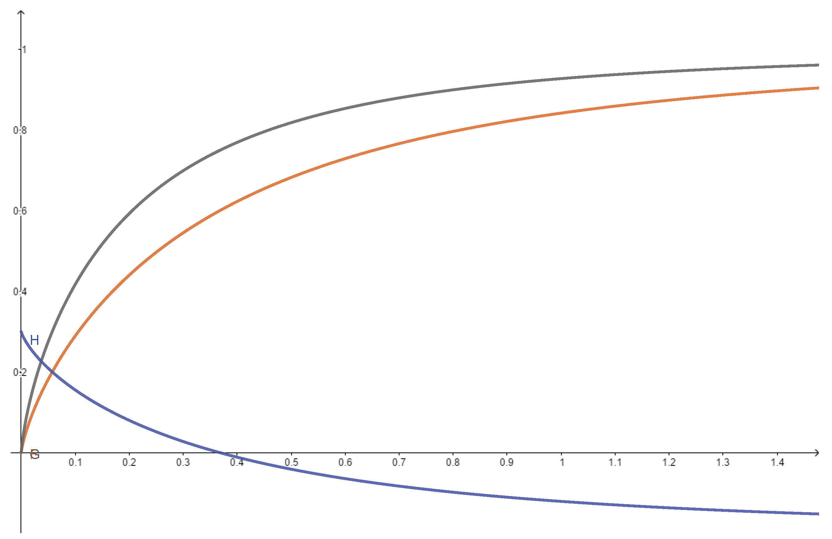
We note that the examples used in Remark 1 also verify conditions $|{\rho }_1(a,b)| < \frac{3}{2},$ and it is illustrated by Figure 1 (see below).

Figure 1. Graphs of the functions F and G (from Remark 1) and H (from Remark 3).

Figure 1. Graphs of the functions F and G (from Remark 1) and H (from Remark 3).

Theorem 7.

Under the assumptions of Theorem 3, the following inequality holds true:

$$\begin{array}{cc}\hfill & \left|\frac{h\left(a\right)+h\left(b\right)}{2}-\frac{1}{b-a}{\int }_a^{b}h\left(x\right)dx\right|\leqq \left|{\rho }_2(a,b)\right|(b-a){\left(\frac{5}{72}\right)}^{1-\frac{1}{q}}\hfill \\ \hfill & ·\left\{{\left(\frac{111|h^{\prime }{\left(a\right)|}^q}{1944}+\frac{|h^{\prime }{\left(b\right)|}^q}{81}\right)}^{\frac{1}{q}}+{\left(\frac{|h^{\prime }{\left(a\right)|}^q}{81}+\frac{111|h^{\prime }{\left(b\right)|}^q}{1944}\right)}^{\frac{1}{q}}\right\},\hfill \end{array}$$

(20)

where

$${\rho }_2(a,b)=:1-\frac{h\left(A(a,b)\right)-A\left(h\left(a\right),h\left(b\right)\right)}{3\mathsf{\Xi }(a,b)}.$$

Proof. 

From Lemma 1, we have

$$\begin{array}{cc}\hfill & \left|\frac{h\left(a\right)+h\left(b\right)}{2}-\frac{1}{b-a}{\int }_a^{b}h\left(x\right)dx\right|\hfill \\ \hfill & =(b-a)|{\int }_0^{\frac{1}{2}}\left(x-\frac{1}{3}\right)h^{\prime }\left(a+x(b-a)\right)dx\hfill \\ \hfill & +{\int }_{\frac{1}{2}}^1\left(x-\frac{2}{3}\right)h^{\prime }\left(a+x(b-a)\right)dx\hfill \\ \hfill & -\frac{h\left(A(a,b)\right)-A\left(h\left(a\right),h\left(b\right)\right)}{3(b-a)}|\hfill \\ \hfill & =(b-a)|{\int }_0^{\frac{1}{2}}\left(x-\frac{1}{3}\right)h^{\prime }\left(a+x(b-a)\right)dx\hfill \\ \hfill & +{\int }_{\frac{1}{2}}^1\left(x-\frac{2}{3}\right)h^{\prime }\left(a+x(b-a)\right)dx|\hfill \\ \hfill & ·\left|1-\frac{h\left(A(a,b)\right)-A\left(h\left(a\right),h\left(b\right)\right)}{3\mathsf{\Xi }(a,b)}\right|.\hfill \end{array}$$

(21)

By repeating the same steps as in the proof of Theorem 3 together with the above relation, we derive the assertion of Theorem 7. Exactly, these steps consist of using integral representation with the derivative $h^{\prime }$ via the arithmetic means (21) and following obvious integral estimates instead of (6), and after that, using the Hölder integral inequality [2] for the cases $q=1$ and $q>1$ one by one. □

Remark 3.

If we take $q=1$ in Theorem 7, we obtain

$$\begin{array}{cc}\hfill & \left|\frac{h\left(a\right)+h\left(b\right)}{2}-\frac{1}{b-a}{\int }_a^{b}h\left(x\right)dx\right|\hfill \\ \hfill & \leqq \frac{5|{\rho }_2(a,b)|(b-a)}{72}\left(|h^{\prime }\left(a\right)|+|h^{\prime }\left(b\right)|\right).\hfill \end{array}$$

(22)

We note that the obtained midpoint inequality (22) is better than the inequality (2) if $|{\rho }_2| < \frac{9}{5}.$ It means that the absolute positive constant at the right-hand side of the inequality (22) is smaller, and so better, than the right-hand side of the inequality (2); so, under the above condition $|{\rho }_2| < \frac{9}{5}$, the inequality (22) is more exact than the inequality (2).

In order to support this observation, we consider the following example: set $h\left(x\right)=\psi \left(x\right)$ and $[a,b]=[t,t+2]t>0.$ In this case, we have

$$h\left(A(t,t+2)\right)-A\left(h\left(t\right),h(t+2)\right)=\frac{1}{2t(t+1)}$$

and

$${\rho }_2(t,t+2)=1-\frac{1}{6t(t+1)\psi \left(t\right)-3t(t+1)log\left(t(t+1)\right)+6t+4}.$$

We set

$$H\left(t\right)=\frac{9}{5}-\left|1-\frac{1}{6t(t+1)\psi \left(t\right)-3t(t+1)log\left(t(t+1)\right)+6t+4}\right|.$$

Figure 1 illustrates that the right-hand side of the inequality (22) is sharper than the right-hand side of the inequality (2) on the interval $[t,t+2]$, where $t\in (0,0.367217).$

Theorem 8.

With the assumptions of Theorem 4, the following inequality holds true:

$$\begin{array}{cc}\hfill & \left|\frac{h\left(a\right)+h\left(b\right)}{2}-\frac{1}{b-a}{\int }_a^{b}h\left(x\right)dx\right|\hfill \\ \hfill & \leqq \frac{(b-a)|{\rho }_2(a,b)|}{12}{\left(\frac{1+2^{p+1}}{3(p+1)}\right)}^{\frac{1}{p}}{\left[|h^{\prime }{\left(a\right)|}^q+{\left|h^{\prime }\left(b\right)\right|}^q\right]}^{\frac{1}{q}}\hfill \end{array}$$

(23)

with

$$\frac{1}{p}+\frac{1}{q}=1.$$

Proof. 

We just repeat the same calculations as in the proof of Theorem 4 using (21). □

On setting $p=q=2$ in (23), we obtain the following consequence.

Corollary 1.

With the conditions of Theorem 4, it is asserted that

$$\begin{array}{cc}\hfill & \left|\frac{h\left(a\right)+h\left(b\right)}{2}-\frac{1}{b-a}{\int }_a^{b}h\left(x\right)dx\right|\hfill \\ \hfill & \leqq \frac{(b-a)|{\rho }_2(a,b)|}{12}\sqrt{|h^{\prime }{\left(a\right)|}^2+{\left|h^{\prime }\left(b\right)\right|}^2}.\hfill \end{array}$$

(24)

Remark 4.

We note that the left-hand side of the inequality (24) is better than the left-hand side of the inequality (2) if $|{\rho }_2| < \frac{3}{2}.$ It means that the absolute positive constant on the right-hand side of the inequality (24) is smaller, and so better, than the right-hand side of the inequality (2). Consequently, under the above condition $|{\rho }_2| < \frac{3}{2},$ the inequality (24) is sharper than the inequality (2).

3. Applications

3.1. Some New Inequalities for the Digamma Function in Terms of the Trigamma Function

Our aim in this section is to establish new inequalities involving the digamma and trigamma functions.

Proposition 1.

For $t>0,$ the next inequality holds true:

$$\left|\psi \left(t\right)-log\left(\sqrt{t(t+1)}\right)+\frac{3t+2}{3t(t+1)}\right|\leqq \frac{5}{72}\left(2{\psi }^{\prime }\left(t\right)-\frac{2t^2+2t+1}{t^2{(t+1)}^2}\right).$$

(25)

Proof. 

Upon setting $h\left(x\right)=\psi \left(x\right)$ and $[a,b]=[t,t+2]$ in Theorem 3 ($q=1$) and using (17), we obtain

$$\left|3\psi \left(t\right)+\frac{2}{t}+\frac{1}{t+1}-\frac{3}{2}log\left(t(t+1)\right)\right|\leqq \frac{5}{24}\left(|{\psi }^{\prime }(t+2)|+|{\psi }^{\prime }\left(t\right)|\right).$$

(26)

Again, by using (17), we have

$${\psi }^{\prime }(t+2)={\psi }^{\prime }\left(t\right)-\frac{1}{t^2}-\frac{1}{{(t+1)}^2}.$$

In view of the above relations and straightforward calculation, we derive the desired inequality (25) asserted by Proposition 1. □

Proposition 2.

For any $t>0,$ the following inequality holds true:

$$\left|2\psi \left(t\right)+\psi \left(t+\frac{1}{2}\right)-3logt+\frac{1}{t}\right|\leqq \frac{5}{24}\left(2{\psi }^{\prime }\left(t\right)+\frac{1}{t}\right).$$

(27)

Proof. 

We set $h\left(x\right)=\psi \left(x\right)$ and $[a,b]=[t,t+1],t>0$ in Theorem 3. The details involved are derived by a straightforward calculation. □

3.2. Applications of Hermite-Hadamard-Type Inequalities to Linear Combinations of Some Special Means

The study of different kinds of means is fulfilled in (for example) [2,25,28,29,30]. It is one of the most important notions in mathematical analysis and its applications.

With the aid of some results in Section 3, our aim in this section is to derive some new inequalities involving combinations of special means and its powers.

As usual, for arbitrary positive real numbers a and b, we define the following items.

• The arithmetic and geometric means given by

  $$A(x,y)=\frac{x+y}{2}\mathrm{and}G(x,y)=\sqrt{ab}.$$
• The logarithmic mean given by

  $$L(a,b)=\frac{b-a}{logb-loga}(a\ne b).$$
• The generalized logarithmic mean given by

  $$L_n(a,b)={\left(\frac{b^{p+1}-a^{p+1}}{(p+1)(b-a)}\right)}^{\frac{1}{p}}\left(p\in \mathbb{R}\backslash \left\{-1,0\right\};a\ne b\right).$$

In fact, the logarithmic mean and a generalized logarithmic mean are special cases of the means introduced by Tibor Radó. Tibor Radó also established several important inequalities for them (see, for details, [2]).

Proposition 3.

Let $r\in (0,1]$ and $a,b\in \mathbb{R}$ such that $0 < a < b.$ Then the following inequality holds true:

$$\begin{array}{cc}\hfill & \left|\frac{2}{3}A(a^r,b^r)+\frac{1}{3}{A}^r(a,b)-L_r^r(a,b)\right|\leqq r(b-a){\left(\frac{5}{72}\right)}^{1-\frac{1}{q}}\hfill \\ \hfill & ·\left\{{\left(\frac{111a^{q(r-1)}}{1944}+\frac{b^{q(r-1)}}{81}\right)}^{\frac{1}{q}}+{\left(\frac{a^{q(r-1)}}{81}+\frac{111b^{q(r-1)}}{1944}\right)}^{\frac{1}{q}}\right\}\hfill \end{array}$$

(28)

for all $q\geqq 1.$

Proof. 

Proposition 3 follows from Theorem 3 upon setting $q=1$ and

$$h\left(x\right)=x^r\left(r\in (0,1]\right).$$

□

Proposition 4.

Under the assumptions of Proposition 3, the following inequalities hold true:

$$\begin{array}{cc}\hfill & \left|\frac{2}{3}A(a^r,b^r)+\frac{1}{3}{A}^r(a,b)-L_r^r(a,b)\right|\hfill \\ \hfill & \leqq \frac{r(b-a)}{6}{\left(\frac{1+2^{p+1}}{6(p+1)}\right)}^{\frac{1}{p}}{A}^{\frac{1}{q}}\left(a^{q(r-1)},b^{q(r-1)}\right),\hfill \end{array}$$

(29)

where

$$\frac{1}{p}+\frac{1}{q}=1(p>1).$$

Proof. 

Proposition 4 follows from Theorem 4 by putting $h\left(x\right)=x^r\left(\alpha \in (0,1]\right).$ □

If we set

$$h\left(x\right)=\frac{1}{x^r}\left(r\in (0,1]\right)$$

in Theorem 3, we deduce the following inequality.

Proposition 5.

With the conditions of Proposition 3, the following result holds true:

$$\begin{array}{cc}\hfill & |\frac{2}{3}A(a^{-r},b^{-r})+\frac{1}{3}{A}^{-r}(a,b)-L_{-r}^{-r}(a,b)|\leqq r(b-a){\left(\frac{5}{72}\right)}^{1-\frac{1}{q}}\hfill \\ \hfill & ·\left\{{\left(\frac{111a^{-q(r+1)}}{1944}+\frac{b^{-q(r+1)}}{81}\right)}^{\frac{1}{q}}+{\left(\frac{a^{-q(r+1)}}{81}+\frac{111b^{-q(r+1)}}{1944}\right)}^{\frac{1}{q}}\right\}\hfill \end{array}$$

(30)

for all $q\geqq 1.$

Remark 5.

If we set$r=1$ in (30), we obtain

$$\begin{array}{cc}\hfill & |\frac{2}{3}A(a^{-1},b^{-1})+\frac{1}{3}{A}^{-1}(a,b)-L_{-1}^{-1}(a,b)|\leqq (b-a){\left(\frac{5}{72}\right)}^{1-\frac{1}{q}}\hfill \\ \hfill & \left\{{\left(\frac{111a^{-2q}}{1944}+\frac{b^{-2q}}{81}\right)}^{\frac{1}{q}}+{\left(\frac{a^{-2q}}{81}+\frac{111b^{-2q}}{1944}\right)}^{\frac{1}{q}}\right\},\hfill \end{array}$$

(31)

where $q\geqq 1.$

Upon setting

$$f\left(t\right)=\frac{1}{t^r}\left(r\in (0,1]\right)$$

in Theorem 4, we get the following inequality.

Proposition 6.

With the assumptions of Proposition 3, the following inequality is valid:

$$\begin{array}{cc}\hfill & |\frac{2}{3}A(a^{-r},b^{-r})+\frac{1}{3}{A}^{-r}(a,b)-L_{-r}^{-r}(a,b)|\hfill \\ \hfill & \leqq \frac{r(b-a)}{6}{\left(\frac{1+2^{p+1}}{6(p+1)}\right)}^{\frac{1}{p}}A\left(a^{-q(r+1)},a^{-q(r+1)}\right)\hfill \end{array}$$

(32)

with

$$\frac{1}{p}+\frac{1}{q}=1\left(min\{p,q\}>1\right).$$

In particular, we obtain

$$\begin{array}{cc}\hfill & |\frac{2}{3}A(a^{-1},b^{-1})+\frac{1}{3}{A}^{-1}(a,b)-L_{-1}^{-1}(a,b)|\hfill \\ \hfill & \leqq \frac{b-a}{6}{\left(\frac{1+2^{p+1}}{6(p+1)}\right)}^{\frac{1}{p}}A\left(a^{-2q},a^{-2q}\right),\hfill \end{array}$$

(33)

where

$$\frac{1}{p}+\frac{1}{q}=1\left(min\{p,q\}>1\right).$$

4. Conclusions

In this paper, we have establishd new Hermite-Hadamard-type inequalities for a class of functions with some convexity conditions on their derivatives. As consequences of some of our main results, we have obtained some new inequalities for the digamma function in terms of the trigamma function. Some applications to special means of real numbers are also given. The analytical and numerical computation show that some of the obtained results are better than the the corresponding known results.

References

- Dragomir, S.S.; Pearce, C.E.M. Selected Topics on Hermite–Hadamard Inequalities and Applications; RGMIA Monograph Series; Victoria University of Technology: Melbourne, Australia, 2003; Available online: https://ssrn.com/abstract=3158351 (accessed on 5 July 2022).
- Mitrinović, D.S.; Peĉarić, J.; Fink, A. Classical and New Inequalities in Analysis; (Eastern European Series on Mathematics and Its Applications); Kluwer Academic Publishers: Dordrecht, The Netherlands, 1993; Volume 61. [Google Scholar]
- Shishkina, E.; Sitnik, S.M. Transmutations, Singular and Fractional Differential Equations with Applications to Mathematical Physics; (Series on Mathematics in Science and Engineering); Academic Press: Cambridge, MA, USA, 2020. [Google Scholar]
- Alomari, M.; Darus, M.; Dragomir, S.S. New inequalities of Hermite–Hadamard type for functions whose second derivates absolute values are quasi-convex. RGMIA Res. Rep. Collect. 2009, 12, 1–5. [Google Scholar]
- Azpeitia, A.G. Convex functions and the Hadamard inequality. Rev. Colomb. Mat. 1994, 28, 7–12. [Google Scholar]
- Bakula, M.K.; Peĉarić, J.E. Note on some Hadamard-type inequalities. J. Inequal. Pure Appl. Math. 2004, 5, 74. [Google Scholar]
- Dragomir, S.S.; Agarwal, R.P. Two inequalities for differentiable mappings and applications to special means of real numbers and to trapezoidal formula. Appl. Math. Lett. 1998, 11, 91–95. [Google Scholar] [CrossRef]
- Dragomir, S.S. On some new inequalities of Hermite-Hadamard type for m-convex functions. Tamkang J. Math. 2002, 33, 45–56. [Google Scholar] [CrossRef]
- Dragomir, S.S. Two mappings in connection to Hadamard’s inequalities. J. Math. Anal. Appl. 1992, 167, 49–56. [Google Scholar] [CrossRef]
- Erden, S.; Sarikaya, M.Z. New Hermite-hadamard type inequalities for twice differentiable convex mappings via green function and applications. Moroccan J. Pure Appl. Anal. 2016, 2, 107–117. [Google Scholar] [CrossRef]
- Kavurmaci, H.; Avci, M.; Özdemir, M.E. New inequalities of hermite-hadamard type for convex functions with applications. J. Inequal. Appl. 2011, 2011, 86. [Google Scholar] [CrossRef]
- Kirmaci, U.S. Inequalities for differentiable mappings and applications to special means of real numbers to midpoint formula. Appl. Math. Comput. 2004, 147, 137–146. [Google Scholar] [CrossRef]
- Kirmaci, U.S.; Bakula, M.K.; Özdemir, M.E.; Peĉarić, J.E. Hadamard-tpye inequalities for s-convex functions. Appl. Math. Comput. 2007, 193, 26–35. [Google Scholar] [CrossRef]
- Pearce, C.E.M.; Peĉarić, J.E. Inequalities for differentiable mappings with application to special means and quadrature formula. Appl. Math. Lett. 2000, 13, 51–55. [Google Scholar] [CrossRef]
- Özdemir, M.E.; Avci, M.; Set, E. On some inequalities of Hermite-Hadamard type via m-convexity. Appl. Math. Lett. 2010, 23, 1065–1070. [Google Scholar] [CrossRef]
- Sarikaya, M.Z.; Set, E.; Özdemir, M.E. On some new inequalities of hadamard-type involving h-convex functions. Acta Math. Univ. Comenian. (N.S.) 2010, 79, 265–272. [Google Scholar]
- Sarikaya, M.Z.; Kiris, M.E. Some new inequalities of Hermite-Hadamard type for s-convex functions. Miskolc Math. Notes 2015, 16, 491–501. [Google Scholar] [CrossRef]
- Set, E.; Özdemir, M.E.; Dragomir, S.S. On the Hermite-Hadamard inequality and other integral inequalities involving two functions. J. Inequal. Appl. 2010, 9, 148102. [Google Scholar] [CrossRef]
- Set, E.; Özdemir, M.E.; Dragomir, S.S. On Hadamard-type inequalities involving several kinds of convexity. J. Inequal. Appl. 2010, 12, 286845. [Google Scholar] [CrossRef]
- Khan, M.B.; Srivastava, H.M.; Mohammed, P.O.; Nonlaopon, K.; Hamed, Y.S. Some new Jensen, Schur and Hermite-Hadamard inequalities for log convex fuzzy interval-valued functions. AIMS Math. 2022, 7, 4338–4358. [Google Scholar] [CrossRef]
- Srivastava, H.M.; Sahoo, S.K.; Mohammed, P.O.; Baleanu, D.; Kodamasingh, B. Hermite-Hadamard type inequalities for interval-valued preinvex functions via fractional integral operators. Internat. J. Comput. Intel. Syst. 2022, 15, 8. [Google Scholar] [CrossRef]
- Khan, M.B.; Srivastava, H.M.; Mohammed, P.O.; Macías-Diaz, J.E.; Hamed, Y.S. Some new versions of integral inequalities for log-preinvex fuzzy-interval-valued functions through fuzzy order relation. Alex. Eng. J. 2022, 61, 7089–7101. [Google Scholar] [CrossRef]
- Srivastava, H.M.; Zhang, Z.-H.; Wu, Y.-D. Some further refinements and extensions of the Hermite-Hadamard and Jensen inequalities in several variables. Math. Comput. Model. 2011, 54, 2709–2717. [Google Scholar] [CrossRef]
- Peĉarić, J.E.; Proschan, F.; Tong, Y.L. Convex Functions, Partial Orderings, and Statistical Applications; Academic Press Incorporated: Cambridge, MA, USA, 1992. [Google Scholar]
- Hardy, G.H.; Littlewood, J.E.; Pólya, G. Inequalities; Cambridge University Press: Cambridge/London, UK; New York, NY, USA, 1952. [Google Scholar]
- Karp, D.; Sitnik, S.M. Log-convexity and log-concavity of hypergeometric-like functions. J. Math. Anal. Appl. 2010, 364, 384–394. [Google Scholar] [CrossRef] [Green Version]
- Niculescu, C.; Persson, L.E. Convex Functions and Their Applications: A Contemporary Approach; Springer: Berlin/Heidelberg, Germany; New York, NY, USA, 2006. [Google Scholar]
- Bullen, P.S.; Mitrinović, D.S.; Vasić, P.M. Means and Their Inequalities; D. Reidel Publishing Company: Dordrecht, The Netherlands, 1988. [Google Scholar]
- Bullen, P.S. Handbook of Means and Their Inequalities; (Kluwer Series on Mathematics and Its Applications); Kluwer Academic Publishers: Dordrecht, The Netherlands, 2003; Volume 560. [Google Scholar]
- Bullen, P.S. Dictionary of Inequalities; (Pitman Monographs and Surveys in Pure and Applied Mathematics); CRC Press: Boca Raton, FL, USA, 1998; Volume 97. [Google Scholar]
Publisher’s Note: MDPI stays neutral with regard to jurisdictional claims in published maps and institutional affiliations. |
© 2022 by the authors. Licensee MDPI, Basel, Switzerland. This article is an open access article distributed under the terms and conditions of the Creative Commons Attribution (CC BY) license (https://creativecommons.org/licenses/by/4.0/).
Share and Cite
MDPI and ACS Style
Srivastava, H.M.; Mehrez, S.; Sitnik, S.M. Hermite-Hadamard-Type Integral Inequalities for Convex Functions and Their Applications. Mathematics 2022, 10, 3127. https://doi.org/10.3390/math10173127
AMA Style
Srivastava HM, Mehrez S, Sitnik SM. Hermite-Hadamard-Type Integral Inequalities for Convex Functions and Their Applications. Mathematics. 2022; 10(17):3127. https://doi.org/10.3390/math10173127
Chicago/Turabian StyleSrivastava, Hari M., Sana Mehrez, and Sergei M. Sitnik. 2022. "Hermite-Hadamard-Type Integral Inequalities for Convex Functions and Their Applications" Mathematics 10, no. 17: 3127. https://doi.org/10.3390/math10173127
Note that from the first issue of 2016, this journal uses article numbers instead of page numbers. See further details here.