

A Topological Machine Learning Pipeline for Classification


1
Department of Mathematics, University of Pisa, 56126 Pisa, Italy
2
Institute of Information Science and Technologies “A. Faedo”, National Research Council of Italy (CNR), 56124 Pisa, Italy
*
Author to whom correspondence should be addressed.
†
These authors contributed equally to this work.
Mathematics 2022, 10(17), 3086; https://doi.org/10.3390/math10173086
Submission received: 24 July 2022
/
Revised: 13 August 2022
/
Accepted: 18 August 2022
/
Published: 27 August 2022
(This article belongs to the Special Issue Computational Algebraic Topology and Neural Networks in Computer Vision)
Abstract
:In this work, we develop a pipeline that associates Persistence Diagrams to digital data via the most appropriate filtration for the type of data considered. Using a grid search approach, this pipeline determines optimal representation methods and parameters. The development of such a topological pipeline for Machine Learning involves two crucial steps that strongly affect its performance: firstly, digital data must be represented as an algebraic object with a proper associated filtration in order to compute its topological summary, the Persistence Diagram. Secondly, the persistence diagram must be transformed with suitable representation methods in order to be introduced in a Machine Learning algorithm. We assess the performance of our pipeline, and in parallel, we compare the different representation methods on popular benchmark datasets. This work is a first step toward both an easy and ready-to-use pipeline for data classification using persistent homology and Machine Learning, and to understand the theoretical reasons why, given a dataset and a task to be performed, a pair (filtration, topological representation) is better than another.
MSC:
55N31; 62R40; 68T051. Introduction
In the last decade, scientific and industrial research has introduced the need to manage huge quantities of digital data. Numerous studies have therefore arisen to provide appropriate tools for such research. In the mathematical field, Topological Data Analysis (TDA) has started to play a major role since it provides qualitative and quantitative features to describe the data space from a geometrical point of view. Topological data analysis has its roots in Persistent Homology (PH), which combines algebraic topology with discrete Morse theory. Informally, algebraic topology studies the global shape of a space by means of features that are invariant under continuous deformation. These features are essentially the number of k-dimensional holes in the space. Persistent homology, on the other hand, studies the evolution of the data space at different scales of resolution and tracks the topological invariants (k-dimensional holes) that form and vanish during this process. These topological invariants encode the global geometrical properties of the data space. The collection of such information is called a Persistent Diagram (PD). The idea of injecting geometric information into Machine Learning (ML) and deep learning is currently a very active field in the scientific community [1,2,3,4,5]. Suffice it to say that convolutional neural networks are part of this research area. The results provided by TDA have proved very promising [4,6,7,8,9]. However, the synergy between TDA and ML is quite novel, since the main concept of TDA, namely Persistence Diagrams, could not be introduced in an ML approach from the get-go. A wide range of transformations have been devised to exploit the capabilities of PDs in ML algorithms [10,11,12,13,14,15,16]. Each of them has been devised with specific requirements. To the best of our knowledge, however, their relative effectiveness in relation to different heterogeneous types of datasets has not been the subject of extensive study. More importantly, the link between the type of data and optimal representation has not yet been addressed. In other words, even if it has been shown in the rich literature on applications of TDA and Machine Learning that topological features are feasible for the classification purposes of several types of data, it is still not clear which is the best way to exploit the topological descriptive power when approaching a new classification task. In addition, a key element of persistent homology is the choice of a filtration that associates a PD with the data. The goal of this work is to investigate the theoretical reasons behind the two main choices that characterize a topological pipeline in relation to a specific goal, namely the choice of filtration and the choice of representation method. Incidentally, we will develop a topological pipeline with different available filtrations and several representation methods with the associated parameters. We will evaluate the results obtained on benchmark datasets and in parallel compare the accuracy of the different representation methods. In doing so, we will lay the groundwork for a correlation between the filtration and vectorization tasks with a particular focus on data type. We emphasize the fact that the purpose of this research is not the classification accuracy of these methods per se but rather to provide a basis for understanding why certain representations are better suited for certain types of data.
2. Mathematical Background
The core idea of our pipeline has its root in Topological Data Analysis (TDA) and Machine Learning (ML). While ML is an already established and well-known branch of artificial intelligence with a wide variety of applications, TDA is a relatively new field of research which studies the geometrical and topological aspects of data. The aim of this work is to emphasize the value of a topological approach in a machine learning context of data analysis. Therefore, a background on Machine Learning will be assumed and will not be recalled in this section nor elsewhere in the article. Conversely, this section is mainly aimed at introducing the reader to topological data analysis and in particular to algebraic topology and persistent homology. Albeit formalities, TDA aims to recognize and analyze patterns within data by means of topology. The main concept of TDA is persistent homology, where the patterns within data are captured across multiple scales. The persistence of a topological feature is the span over different scales of its detectability, and it is an indication of its importance. The collection of such persistences is called the Persistence Diagram.
2.1. Algebraic Topology
Algebraic topology is the mathematical field which aims to study topological spaces by means of algebraic features that are invariant under continuous deformation. Algebraic topology is a wide mathematical field and only a part of it will be relevant in TDA; therefore, this subsection is only a brief introduction to its main concepts. For a more complete guide to algebraic topology, we refer the reader to [17]. The main concept of algebraic topology that we are going to use is the homology of a space, which associates to a topological space a sequence of algebraic objects, namely Abelian groups or modules. More formally, the k-th homology group of a topological space X over a field is a vector space over which we denote as . Beyond the technicalities of its definition, the rank of corresponds to the number of distinct k-dimensional holes in the topological space X, with the exception of . In this case, corresponds to the number of 0-dimensional holes plus one, that is, the number of connected components. Other types of homology can be defined: see reduced homology, relative homology and cohomology. Their definition and use are beyond the scope of this work, so they will not be addressed. In general, different choices of will result in different homology groups . In this work, we limit ourselves to the case where . As an example, Figure 1a shows that the sphere bounds a 2-dimensional void. is connected and there is no 1-dimensional hole. The homology groups for the sphere are:
As another example, Figure 1b shows that the torus is connected, it bounds two 1-dimensional holes (the ones inside the blue and the red loop) and a one 2-dimensional hole. The homology groups for the torus are:
Algebraic topology is a powerful tool that classifies topological spaces with just a finite sequence of integers. The computation for generic topological spaces requires complicated homology and cohomology theories. Persistent homology is now introduced because it enhances the expressiveness of the topological features and it allows easier computation of the homology ranks by means of simplicial homology.
2.2. Persistent Homology
Persistent homology studies the geometry of spaces by looking at the evolution of k-dimensional holes at different spatial resolutions. The key difference with algebraic topology is that the ranks of the homology groups are computed at various scales and the features we extract are precisely the evolution of such ranks [6,18]. This section is only a brief introduction to persistent homology, as many of its concepts will be covered and expanded upon later when we make actual use in the pipeline. Before continuing, it is necessary to introduce the concept of a simplicial complex. Let be affinely independent points. A k-simplex is the convex hull of V, which is called the set of vertices of . We call the face of the convex hull of any subset of points of V and we write when is a face of . A simplicial complex is a set of simplexes such that ; for every and every , it holds that and the intersection of any two simplexes of is always a face of both. A triangulation of a topological space X is a couple where is a simplicial complex and is a homeomorphism. What makes simplicial complexes particularly suitable for our study is that the computation of their homology groups is very simple compared to normal topological spaces. In addition, almost all topological spaces found in practice are triangulable. The ranks of the homology groups of simplicial complexes are more commonly known as Betti numbers. The computation of homology groups and their ranks specifically for simplicial complexes is known as simplicial homology. For more information on simplicial complexes, simplicial homology and the triangulation of topological spaces, we refer the reader to [17]. A filtration of a simplicial complex is a finite sequence of subcomplexes such that . Persistent homology keeps track of changes in the Betti numbers associated to each homology group of for . The persistence of a topological feature is thus its detectability at different spatial resolutions. In particular, features with high persistence will be important to describe the shape of the data, while those with low persistence will be assimilated to noise. The collection of such features is called a Persistence Diagram. To better understand the differences between persistent homology and algebraic topology, we provide the following example. Suppose we have a normal ball and a ball-shaped sponge, which is of course full of many small holes. The difference between these two objects will be detectable or not depending on the resolution at which we are looking at them. If we are looking at them from a distance, the two objects will be indistinguishable. If we look at them close up, we will see the differences. Moreover, the holes will have limited persistence. Therefore, thanks to persistent homology, we can conclude that the two objects have the same shape, but one is basically the noisy version of the other. Not only PH provides algebraic topology with easy tools to compute but it also solves the two main problems associated with digital data, namely their discrete and noisy nature. With regard to the discrete nature, PH allows associating a structure of simplicial complex to discrete data through the filtration. In this way, non-trivial homology groups can be found. As for the noisy nature, PH highlights the most persistent structures at different scales, limiting the incidence of noise.
3. Topological Pipeline
The goal of this section is to define and describe the pipeline we use for the topological study of digital data in a Machine Learning context. As already mentioned, we rely heavily on the tools provided by persistent homology, which will be explored and discussed here. Figure 2 shows the general scheme of our pipeline and its main elements. The digital data (Section 3.1) are filtered (Section 3.2) in order to generate a Persistence Diagram (Section 3.3). We vectorize the PD by means of a vectorization method (Section 3.4). Finally, the collection of all vectors is the input for a Machine Learning classifier (Section 3.5). Figure 3 shows an application of the pipeline to digital data.
3.1. Data
In PH, data are often modeled as points in a metric space or as functions on some topological space. This is straightforward, as the most common digital data found in applications are either n-dimensional vectors or signals and images. Digital data are suitable for modeling both. For example, a grayscale image can be viewed either as a function with domain a grid with values in , or as a vector (a point) in the space . We want to emphasize, however, that the way in which we model data is of fundamental importance for the study that follows. This is mainly due to the type of metrics that the data inherit from the two types of modeling. Continuing our example, the classical metric between two points of is the Euclidean one, while between two functions, we have , or others. Although the metrics can easily be changed according to the context, the different modeling has profound repercussions both mathematically and in terms of application. There is a very rich literature on both the modeling data as points in a metric space [6,19,20] and modeling as functions [4,21,22]. Depending on the type of data, one modeling may be preferred to another. Let us now describe the digital data types we studied in Section 4 and the associated preferred modeling.
3.1.1. Point Cloud Data
Point cloud data are finite metric spaces . We recall that finite metric spaces are naturally equipped with the discrete topology, and the topological dimension of any discrete space is 0. Since every finite metric space is discrete, point clouds do not inherit a (not trivial) topology. As a consequence, the homology of a point cloud is always trivial with the exception of . As finite metric spaces, the natural modeling of this type of data is that of a vector embedded in a larger Euclidean space . Typically, and d is the Euclidean metric, but this model is suitable for generalization. In Section 4, we will always have .
3.1.2. Images
A digital image is an image composed of pixels. In standard 8-bit grayscale images, each pixel has a discrete value ranging from 0 to 255 representing its grayscale intensity. Although it can be considered as a vector of dimension , where the grayscale image has size , modeling an image as a function is preferable. This kind of modeling takes into account the fact that only close pixels can be connected, not also distant ones. Therefore, a digital image is a function from a grid to a suitable finite interval of , depending on the number of channels of the image. The most common number of channels is 1, for grayscale, or 3, for color images. However, there exist additional image channel encodings available.
3.1.3. Graphs
Graphs are structures made by a set of vertices which are connected by edges. There is a distinction between undirected graphs, where the edges link two vertices symmetrically, and directed graphs, where the link is not symmetrical. Another distinction is between weighted and unweighted graphs. More specifically, a graph is an ordered pair where V is the set of vertices and . Typically, , but this is not always the case. A graph is seen as a function with domain E and codomain .
3.2. Filtrations
Persistent homology examines the shape of the data at different scales. As already mentioned in Section 2.2, this means that at each scale j, the data are represented as a simplicial complex . Formally, a filtration of a simplicial complex is a finite sequence of nested subcomplexes
The inclusion induces a homomorphism of the simplicial homology groups for each dimension p and each . Usually, these homomorphisms are actually isomorphisms. In these cases, no topological events have occured between time i and time j and, more importantly, Betti numbers do not change. However, there are cases in which these homomorphisms are not injective or surjective. In these cases, topological events occur, which is precisely what we are interested in. We say that a new topological feature is born at time j when the homomorphism is not surjective. We say that a topological feature dies at time j when the homomorphism is not injective. We keep track of the pairs (birth, death) of the topological features and collect them in the so-called Persistence Diagram (PD).
We would like to focus on the importance of filtrations in our study, as the choice of the filtration is the first fundamental step in a topological study of the data. There are several filtrations available, and they are mainly related to the choice of data modeling. We want to stress that different filtrations yield different topological features and thus possibly very different PDs. Moreover, some filtrations enable emphasizing points with greater or lesser persistence, or they prevent the creation of certain features where there should be none. Therefore, the choice of filtration should be made with caution.
3.2.1. Filtration for Point Clouds
The alpha complex is a way of forming abstract simplicial complexes from a set of points. Hence, it represents an ideal filtration for point clouds. Let be a point cloud embedded in a larger metric space . The elements of X are the vertices of the alpha complex. Fixing a real parameter , we define
That is, we grow balls with radius centered in each point of X, which is intersected with the Voronoi cell of each point. When n and sets intersect, a -simplex is added to the simplicial complex. The growing of naturally induces a filtration. For more information on alpha complex, see [23]. We point out that by the nerve lemma, the alpha complex is homotopically equivalent to the union of the balls and also to the Čech complex. The advantage over the Čech complex is that it is significantly smaller, thus reducing the computational cost.
3.2.2. Filtration for Images
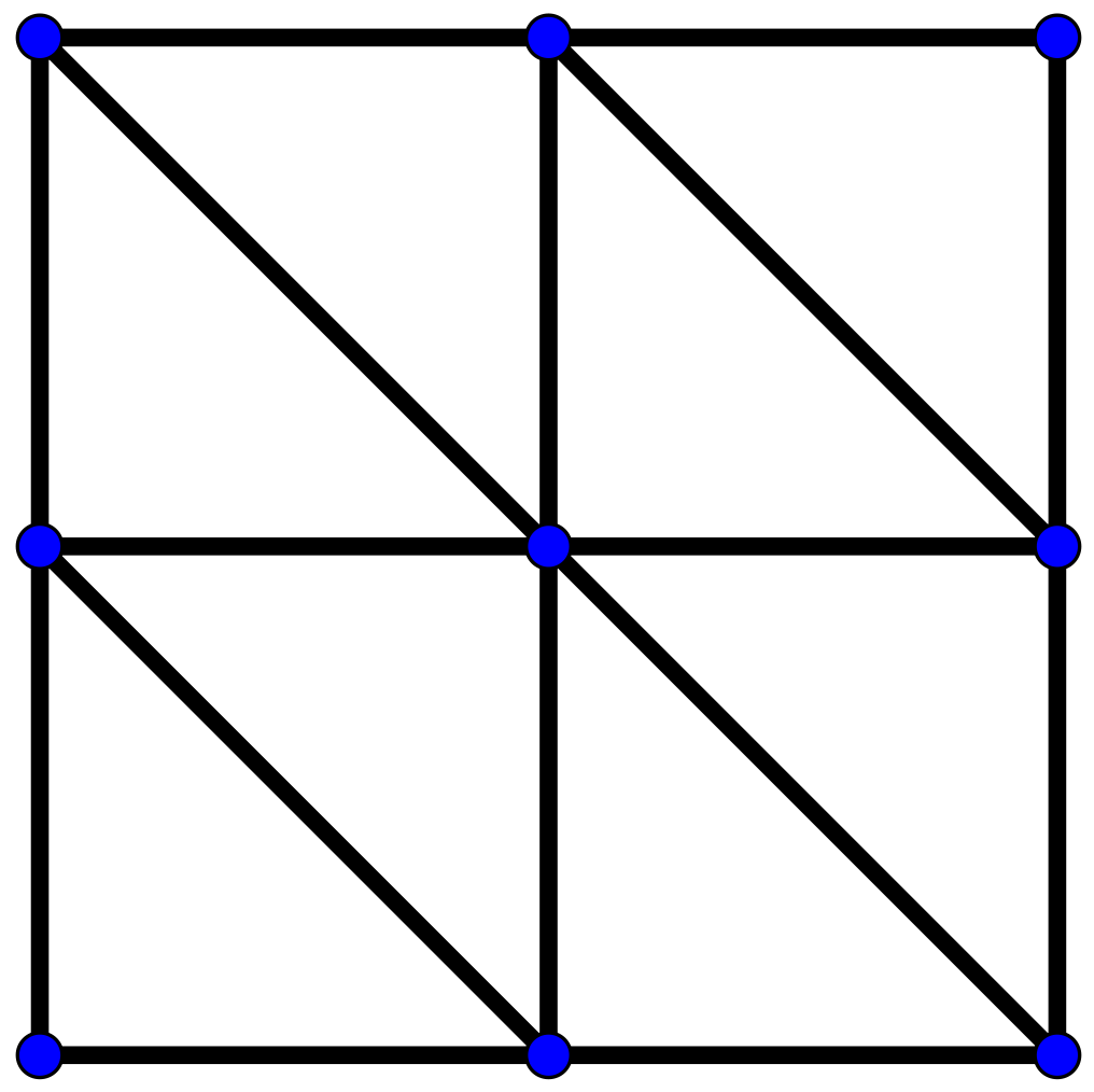
The alpha complex is still a viable filtration for images, since they can be interpreted as vectors. However, other approaches that make greater use of the fixed structure of the image are preferable. In particular, the cubical complex is the ideal filtration as it exploits two key features of images. The first feature is that not all pixels should be connected with each other but only with the neighbors. Figure 4 shows the possible connection between pixels in a cubical complex. The second feature is related to the modeling of images as functions. In contrast to the alpha complex, where all points were immediately inserted as vertices of the simplicial complex, a pixel becomes a vertex of the simplicial complex only when its intensity becomes greater than a certain threshold value t. Similarly, a 1-simplex is added only if two adjacent pixels (in the sense of Figure 4) both have intensities greater than t. The same applies to the 2-simplexes. As t increases, we obtain a filtration. More formally, an elementary cube is any translation of a unit cube embedded in Euclidean space , for some with . A set is a cubical complex if it is homeomorphic to a union of elementary cubes. For more information about cubical complexes, we refer the reader to [24].
3.2.3. Filtration for Graphs
Graphs are particular structures which require ad hoc filtrations. In particular, graphs share many similarities with point clouds but with few key differences. The main difference is that vertices may not be connected to each other. Therefore, no matter how much you increase the filtration value, some 1-simplexes will never be created. This of course impacts also higher-dimensional simplexes. Another difference is that all vertices form 0-simplexes, but their filtration value may not be 0. For example, the number of incident edges of every vertex could be used as a filtration value. There are many possible filtrations associated with graphs, depending mainly on the type of graph considered. In any case, the difference lies essentially in the filtration value associated with each simplex not in the creation of the simplexes themselves. For this reason, we now describe how the simplexes enter the filtration, postponing the description of the filtration value chosen to the Section 4.4. Every vertex forms a 0-simplex. If two vertices are connected by an edge, a 1-simplex is formed. Similarly, when three vertices are pairwise linked, a 2-simplex is formed. In general, a clique is a subset of V whose vertices are all pairwise connected. Each clique of k vertices forms a -simplex.
3.3. Persistence Diagrams
Persistence Diagrams are the collection of pairs (birth, death) of topological features emerged by filtering a simplicial complex. We refer to these pairs as , where is the birth of the jth k-dimensional hole and is its death. Mathematically, this collection is a multiset, that is, a set in which the same elements can appear multiple times. For further details on Persistence Diagrams, we refer the reader to [25,26,27]. Each pair has a multiplicity indicating how many holes share both the birth and the death time. The points of the diagonal are added to the dipersistence diagram with infinite multiplicity for technical reasons. Since the death of a topological feature occurs at a larger time than its birth, PDs are multiset over the set . It holds that if and only if , where and D is a Persistence Diagram. The equality means that the point corresponds to a feature in . We can equip the space of Persistence Diagrams with the bottleneck distance (also called matching distance)
where are Persistence Diagrams and is a bijection from D to . Another popular metric in the space of PDs is the p-Wasserstein distance, which is defined as
For more information on bottleneck and Wasserstein distance, we refer the reader to [27,28]. We point out that in the general case, there exists a bijection only because we have added the points in the diagonal with infinite multiplicity. The most important property of PDs is their stability. That is, a small perturbation of the simplicial complex yields a small perturbation of the associated PD. This property is of fundamental importance in applications as it guarantees robustness against noise and repeatability. Multisets lack fundamental mathematical and statistical properties required in a Machine Learning context, and therefore, they cannot be directly processed by an ML algorithm. To give an example, the mean of two multisets is not well defined. The suitable transformation of PDs into objects that enjoy excellent mathematical properties and can be used in ML is needed. These transformations are called representation methods or featurization methods. We limit our study to the vectorization methods, i.e., procedures for transforming a Persistence Diagram into a vector. Additional representation methods are currently available, i.e., kernel methods. Due to the high computational cost of these methods, they have been omitted from this work, but the interested reader can find more information in [14,15,16].
3.4. Vectorization Methods
A vector representation of a PD consists of an embedding of the space of PD in a vector space or, more generally, in a Hilbert space. The fundamental requirement of this embedding is stability, i.e., that small perturbations of the PD correspond to small perturbations of the associated vector. Various embeddings are obviously possible, and each of them will define a different vector representation of the PD. The vector representations presented in this work are all stable with respect to the bottleneck distance or 1-Wasserstein distance with the exception of Betti curves (see Section 3.4.4). Finally, we want to stress the fact that all these vectors live in a vector space and thus enjoy mathematical and statistical properties that were not available to the space of multisets. Hence, they can be directly introduced in a Machine Learning method. Nonetheless, different representations of the same PD yield different vectors with possible very different results in an ML algorithm. We point out that this is precisely the main goal of this work: to find a correlation between task, filtration and representation. All the subsequent methods require a change of coordinates of the PD. Henceforth, unless otherwise specified, a point will have coordinates , where are the usual birth and death of a topological feature. We point out that in , there is always a connected component that never dies. Since these methods do not handle the infinite persistence of some points, we replace the infinite value by a very large one in relation to the other persistences obtained. Each of these methods is derived from the Gudhi library. For more information about Gudhi and the Python implementation of these methods, we refer the reader to [29].
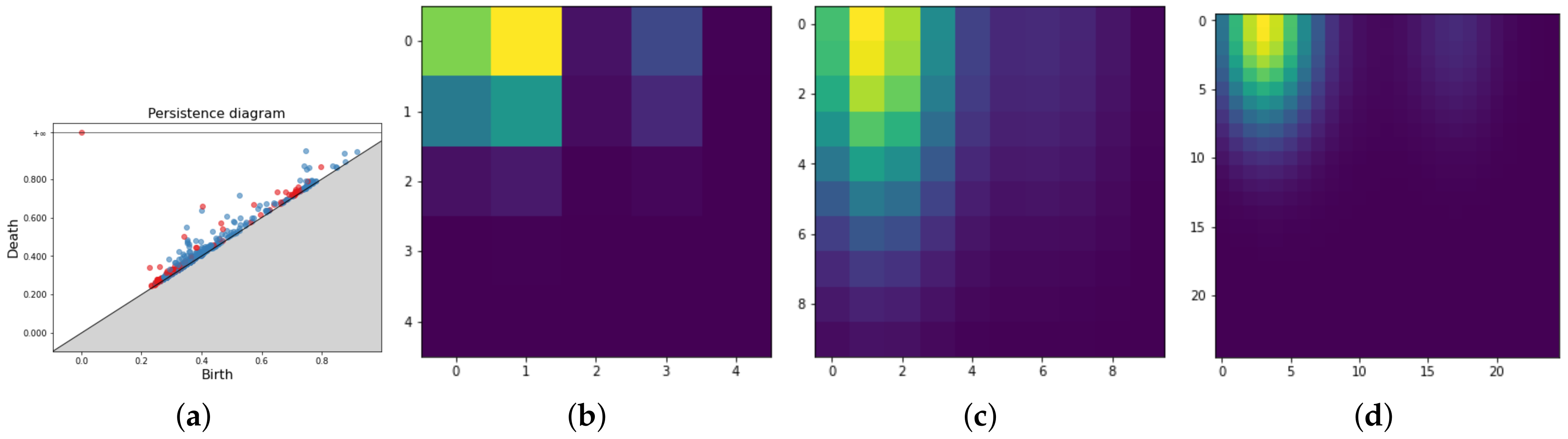
3.4.1. Persistence Image
A Persistence Image (PI) is a finite-dimensional vector representation of Persistence Diagrams. For more information on PI, we refer the reader to [13]. This method basically divides the PD domain into an grid and, for each point q of the PD, defines a Gaussian centered in q with variance . It returns an image where the intensity of each pixel is given by the sum of the values of all Gaussians at that point in the grid, which is weighted by an appropriate function f that must be 0 on the diagonal, continuous and piecewise differentiable. Denoting with m the persistence value of the most persistent feature, the weight function is
The parameters of the method are n and and will be selected by grid search. Figure 5 shows a Persistence Diagram and three different PIs for various parameters. It is evident how different parameter values greatly influence the resulting image. In our pipeline, we determine the optimal parameters with a grid search approach between the following setup: .
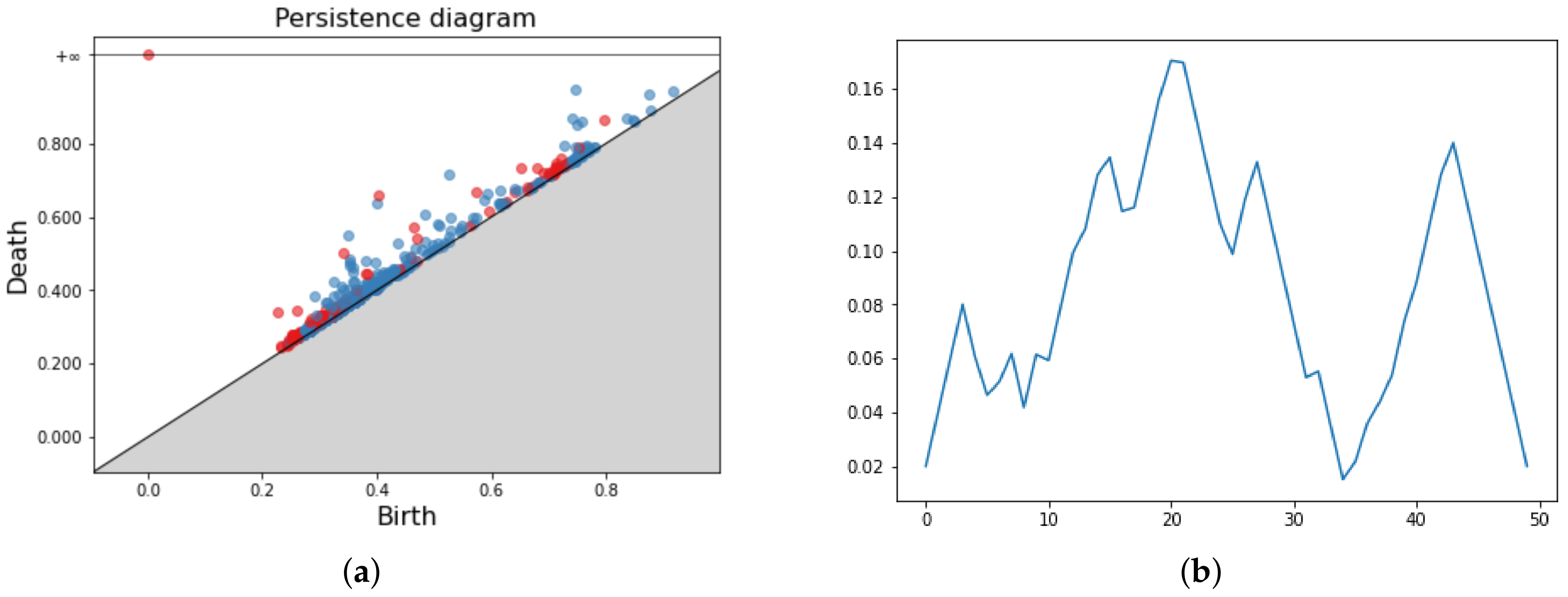
3.4.2. Persistence Landscape
The Persistence Landscape (PL) is another method of vector representation of PD that enjoys excellent statistical properties introduced in [11]. In particular, the PL is a function that lives in a vector space, which is a great mathematical environment for working with ML. More formally, PLs are piecewise constant functions . To define , we tent each persistence point to the baseline with the following function
The Persistence Landscape of D is the collection of such functions
where kmax is the k-th largest value in the set and T is a real number such that for any death time d of a topological feature. Since is piecewise constant, it can be discretized by looking only at the point at which it changes value. This discrete function is the vector representation of the PD. A central limit theorem for PLs holds. The parameters for Persistence Landscapes are the number of landscapes considered n and the discretization resolution r. In our grid search approach, we consider the following setup: . Figure 6 shows a PD and three Persistence Landscapes associated.
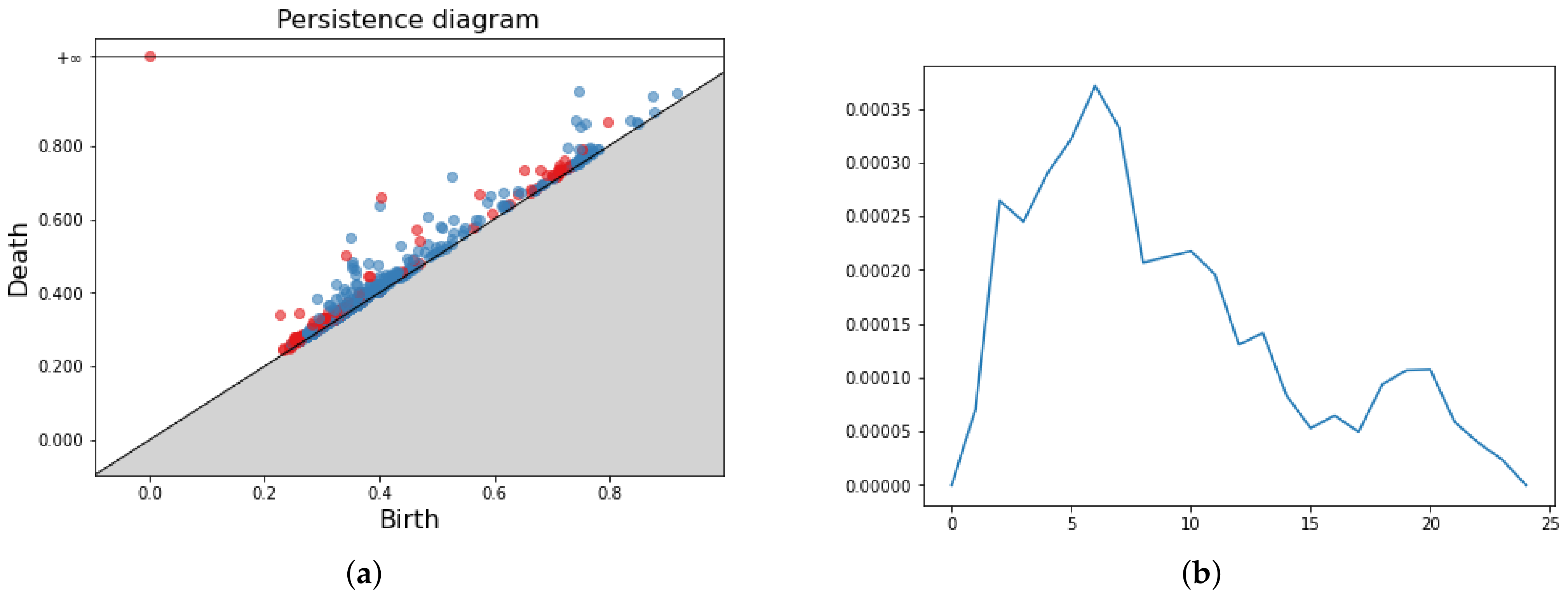
3.4.3. Persistence Silhouette
The Persistence Silhouette (PS) is a method of vector representation of PD with the same core idea of PL. More specifically, it is a piecewise constant function defined as
where m is the number of off-diagonal points, is a weight and is the same function as in Section 3.4.2. Again, the vector representation of the PD comes from the discretization of . In our pipeline, we use constant weight for every . The only parameter of the method is the resolution r, and the grid search takes values . Figure 7 shows a PD and three Persistence Silhouettes. We point out the similarity of the vectors with different parameters values. For more information on Persistence Silhouette, we refer the reader to [10].
3.4.4. Betti Curve
The Betti curve (BC) is yet another vectorization method for Persistence Diagrams presented in [12]. The Betti curve is a -indexed family of functions defined as , where means that q is a topological event in the homology group . The function is then vectorized over a uniform grid of a closed interval and resolution r. For those familiar with persistence barcodes, this method informally counts the number of bars present in the persistence barcodes at any given time after an appropriate persistence normalization. The resolution r in our pipeline takes values in the grid . Figure 8 shows a PD and three BCs for different resolutions of the grid.
In a Persistence Diagram, all points of the different homology dimensions are present. However, some of these dimensions may be more or less suitable for the given study. For this reason, our pipeline follows three approaches. The first approach is to consider each homology group individually. We highlight the fact that it may happen that of some data are empty, for , while others are non-empty. In such cases, we replace the empty with the single point . In the following sections, this approach will be referred to as the approach, for i varying in the homology groups available. The second approach is to forget about the homology dimension of the points, which is referred to as the ‘fused’ approach, whereas the third is to concatenate the vector representation of the PD for each homology dimension, which is referred to as the ‘concat’ approach.
We want to emphasize here that there is no homogeneity in the number of parameters used in the grid search of the various vectorization methods. In particular, Persistence Images have a total of nine parameter combinations, while the others only have four. On the one hand, this maintains a comparison with other works; on the other hand, it is because we are not interested in finding the best vector representation but rather in finding links between data and vectorization methods. Moreover, some methods are more flexible than others and therefore more parameter-dependent. Hence, in these cases, it is more suitable to test a larger number of parameters. Finally, we stress that the purpose of our study is to verify the usefulness of a topological study of the data and to investigate the preferred vector representation in certain contexts. The stability of the representation is of fundamental importance as it guarantees a stable synergy between TDA and ML.
3.5. Machine Learning Classifiers
At this point, we are finally able to introduce the vectorization of the PDs in Machine Learning classifiers. We want to emphasize that the pipeline does not perform parameter tuning either for representation methods or for classifiers. We would also point out that the vector generated from the previous section may have very different sizes and necessarily different computational costs, but this aspect is not taken into account in our experiments. In the pipeline, a total of nine classifiers are trained for each representation. Such classifiers are: Support Vector Classifiers (SVC) with kernel RBF and C = ; a random forest classifier (#trees = 100); and Lasso ().
These classifiers are very standard in Machine Learning literature, and we have reported the parameters used for each of them. For more details, we refer the reader to [30,31,32,33]. Each of these classifiers is derived from the Scikit-learn library. For more information about Scikit-learn and the Python implementation of these methods, we refer the reader to [34]. We want to emphasize that there are such a large number of SVCs just for comparison with other works. Each of the classifiers will perform a 10-fold cross-validation [35] on the data, and we will report the best result obtained for each run along with the representation method that achieved it. We stress the fact that for each run, we report the best accuracy result achieved regardless of the vectorization method or classifier that achieved it. For completeness, we also provide a table with the (mean) accuracy result of the best single method at the end of each experiment. Finally, a statistical analysis of the results obtained during the experiments was carried out and presented in Section 5.
3.6. Further Improvements
The pipeline described up to this point is the basic version of our procedure. It is worth pointing out that this pipeline may have high requirements in terms of time and memory: for example, our pipeline needs a few seconds to classify a sample dynamic trajectory, while it could take about an hour for classifying a complex sample of a collaboration network. This is a basic version because we are omitting some possible improvements in the two main contexts of the pipeline, TDA and ML. For example, multiple filtrations could be available for the same type of data, or more advanced ML methods such as ensemble learning could be used. Since our goal is to take a first step in the study of the best PD representations for different types of digital data, these improvements are initially omitted from the pipeline. If, however, the results obtained are not satisfactory in terms of accuracy and/or stability, suitable improvements will be made. In particular, we stress the fact that the stability of the representation is our most important concern, and high accuracy results without stability are not satisfactory. Necessarily, however, poor but stable results will be equally unsatisfactory. These adjustments to the basic pipeline will be discussed in detail when introduced, as they are strongly linked to the type of dataset considered.
4. Results
In this section, we are going to apply the pipeline presented in Section 3 to different heterogeneous types of datasets. The goal of this section is to discuss the usefulness of a topological study of the data. This is accomplished by showcasing the excellent accuracy results achieved by the pipeline. All results reported here refer to test accuracy. For each dataset, we perform a 10-split cross-validation with training data and test data, and we report the results of the pipeline over the course of the ten runs along with mean accuracy and standard deviation. Finally, since when we have a never-seen data, we would like to know how to perform classification, we also report the accuracy value of the single best method for each dataset (i.e., the best combination {vectorization, classifier}).
4.1. Dynamic Dataset
The first dataset we describe comes from data arising from a discrete dynamical system modeling fluid flow. The dynamical system here presented is a linked twisted map, which is a Poincaré section of an eggbeater-type flow. A Poincaré section is the discretization of a continuous dynamical system obtained by following the path of a particle’s location at discrete time intervals. The equations for the linked twisted map are:
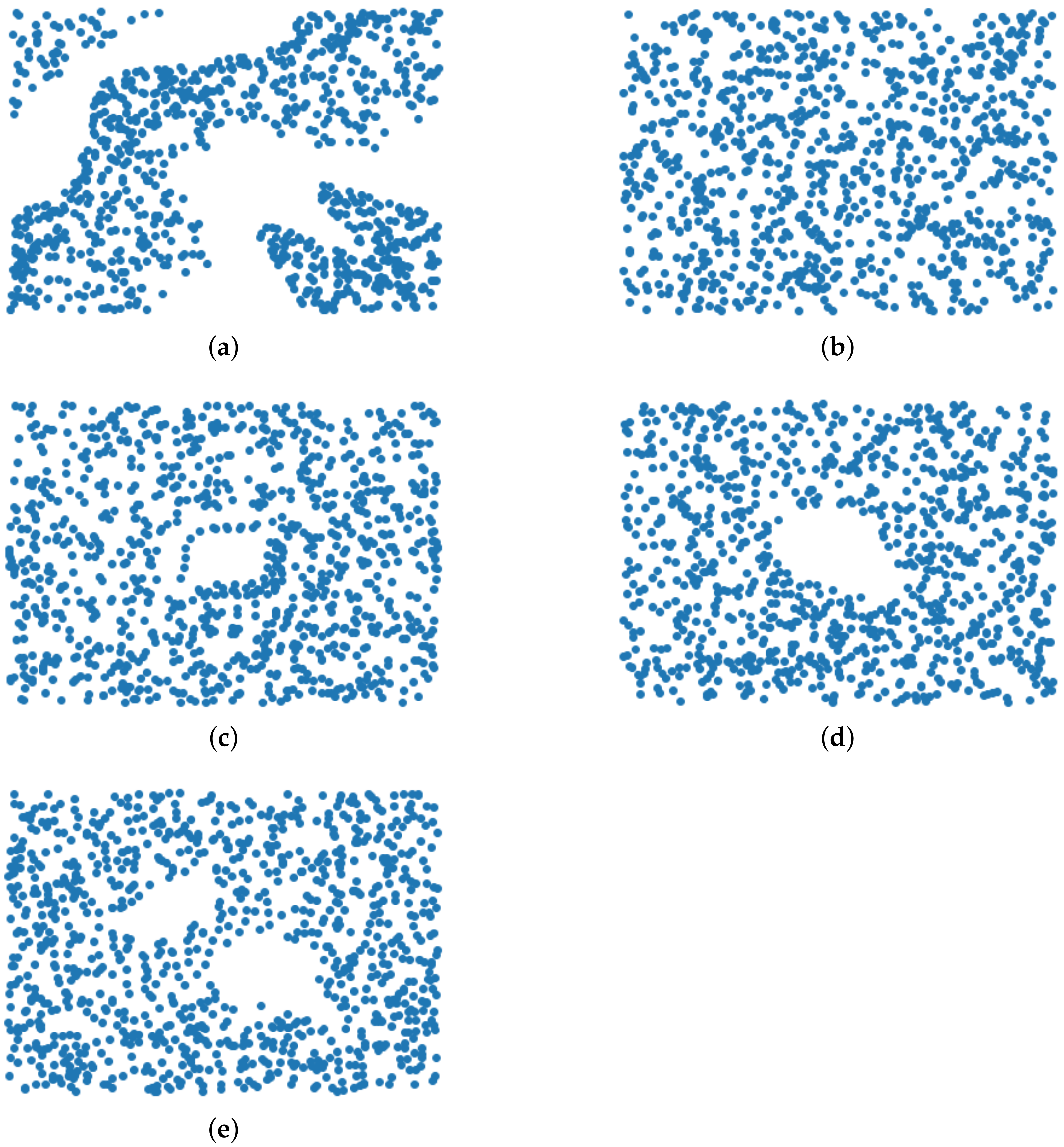
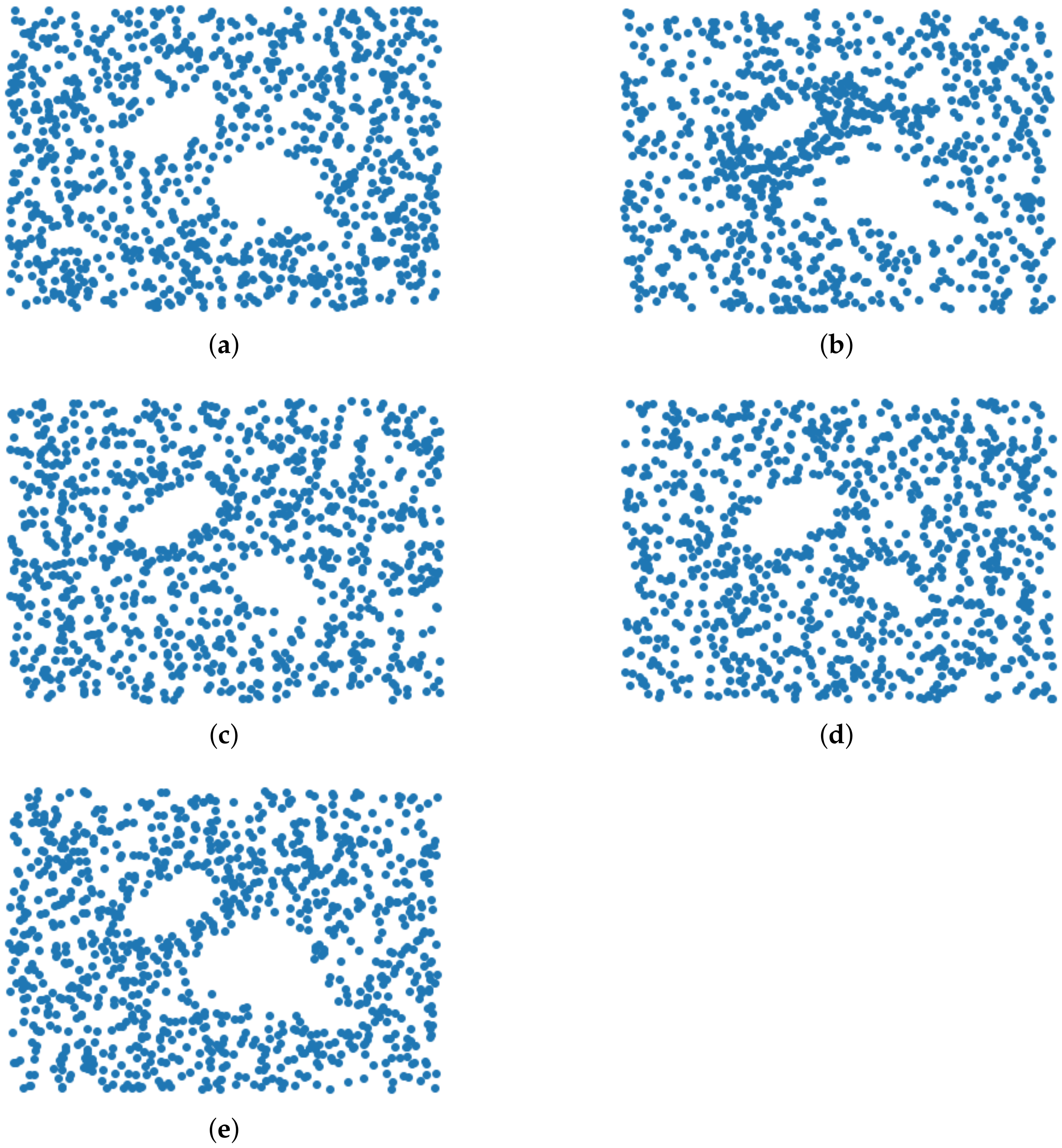
where r is a positive parameter. For different values of the parameter r, different orbits are generated. In some cases, such orbits are dense in the domain ; in other cases, voids occur. The task of this application is to classify the value of the parameter r based on the orbit. In Figure 9, five different orbits generated by the same starting point for five different values of the parameter r are shown. It is clear how the value of r strongly influences the orbit and in particular the formation of voids. In Figure 10, five orbits for the same parameter r with different starting points are shown, clarifying that the shape of the orbit depends only on the value of the parameter r and not on the starting point. This dataset is inspired by [13,36] and is composed of five different values of the parameter , each with 50 orbits generated from different random starting points, for a total of 250 orbits. Each orbit consists of 1000 points generated from 1000 iterations of the linked twisted map. We split the dataset into an training set and test set. The dataset is naturally a point cloud; therefore, the alpha filtration is best suited to generate the PDs. We recall that the pipeline performs a grid search between the most classical representation techniques for Persistence Diagrams, such as Persistence Images or Persistence Landscapes, for different values of the parameters. Such methods are evaluated with a ten-split cross-validation, and the best results are returned. We report in Table 1 the accuracy results obtained by the pipeline for each of the ten runs alongside the abbreviation of the best representation method (PI for Persistence Image and so on). It is worth noticing that the results show a good consistency of the best representation method. As already stated, consistency is of great importance to us, as it demonstrates the feasibility of a single method for classification. The last row reports the mean ± standard deviation of the pipeline over the course of the ten runs. Finally, Table 2 reports the best mean accuracy of the best single method: that is, the combination vectorization method and classifier. Of course, the accuracy of a single method is lower than the mean in Table 1, since in that case, the best accuracy could be achieved by different methods in the various runs. In conclusion, the results obtained by the pipeline in the dynamic dataset are very satisfactory both from the point of view of accuracy and consistency of the representations.
4.2. Mnist
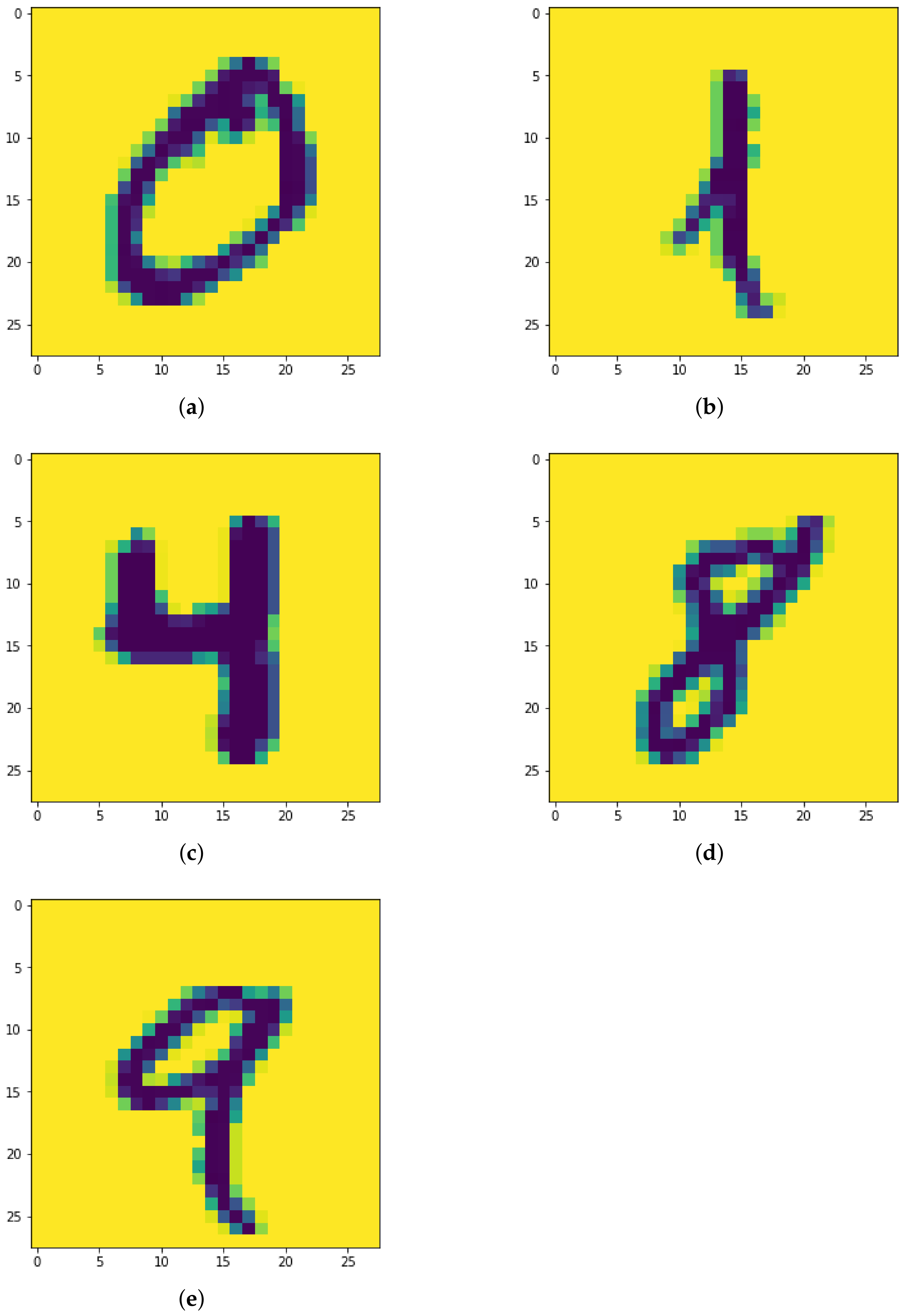
The MNIST dataset is a large dataset of handwritten digits. For more information about the MNIST dataset, we refer the reader to [37], but it basically consists of pixel grayscale images representing digits, and the task is to classify each image to the corresponding digit. Figure 11 shows sample images from the MNIST dataset. To limit the computational cost of this application, only a subsample composed of 5000 training images and 1250 test images is used, following the same train–test ratio as in Section 4.1. In our first, somewhat naive, approach, we directly apply the pipeline to the PDs generated by a grayscale filtration of a normalized and negative image. The negativization of the image is needed in order to focus on the digit instead of the background. For example, in Figure 11d, the digit “8” topologically is one connected component and two 1-cycles. In the negative image, this is exactly what is computed by the pipeline. In the raw image instead are detected three connected components (the three yellow parts) and only one 1-cycle. This behavior is due to the fact that the grayscale filtration is a sublevel filtration, and so the interesting parts of the image should have low intensity. In Table 3, we report the results achieved, and it is clear how they are not at all satisfactory. This behavior is not entirely unexpected, since the homology of handwritten digits is almost always trivial, with few exceptions. As discussed in Section 3.6, we are now going to introduce some improvements to the basic pipeline in order to achieve better results. The grayscale filtration cannot necessarily capture the difference between various digits, as their homology is similar. A switch of filtration is therefore necessary. Following [38], we introduce the height filtration, the radial filtration and the density filtration. All these filtrations capture topological features different from grayscale filtration, which simply captures the global feature of the image. We want to stress that height filtration, radial filtration and density filtration require a binarization of the image in order to be applied. The binarization of the image must be handled carefully for mainly two reasons. The first reason is the inevitable loss of topological features during this process. The second reason is the (arbitrary) choice of the threshold, which could not be obvious a priori. Nonetheless, the MNIST dataset seems particularly suited for binarization, and a trivial threshold of will work just fine. We stress that despite being referred to as filtrations, this is in fact an abuse of notation, as they are not actually filtrations in the sense of Section 3.2. The following filtrations are a mere manipulation of the binarized input image, and they return an image of the same dimensions. There is no persistent homology component that defines a simplicial complex to the given image. In fact, the usual cubical persistence is applied to these filtered images as well. The key difference is that the filtered images have filtration values that emphasize certain topological components.
4.2.1. Height Filtration
The height filtration detects the emergence of topological features by looking at images only along certain directions. The birth and death value of the features is therefore linked to their position in the image and not only to the intensity of the pixels. This is a great improvement in the case of digits, as for example along the direction , the 1-cycle of the digit “6” will have a low birth value, while in the case of the digit “9”, the 1-cycle will have higher birth value and thus different PDs. With the grayscale filtration, both digits would result in one connected component and one 1-cycle, and their persistence would only be determined by the thickness of the loop. For technical reasons, linked to how the height filtration algorithm handles the images, it is not necessary to use the negative of the images. We now describe in more detail the height filtration, presented in [38,39]. Let be a binary image and with . We denote with the Euclidean inner product. The height filtration of and direction v is defined by
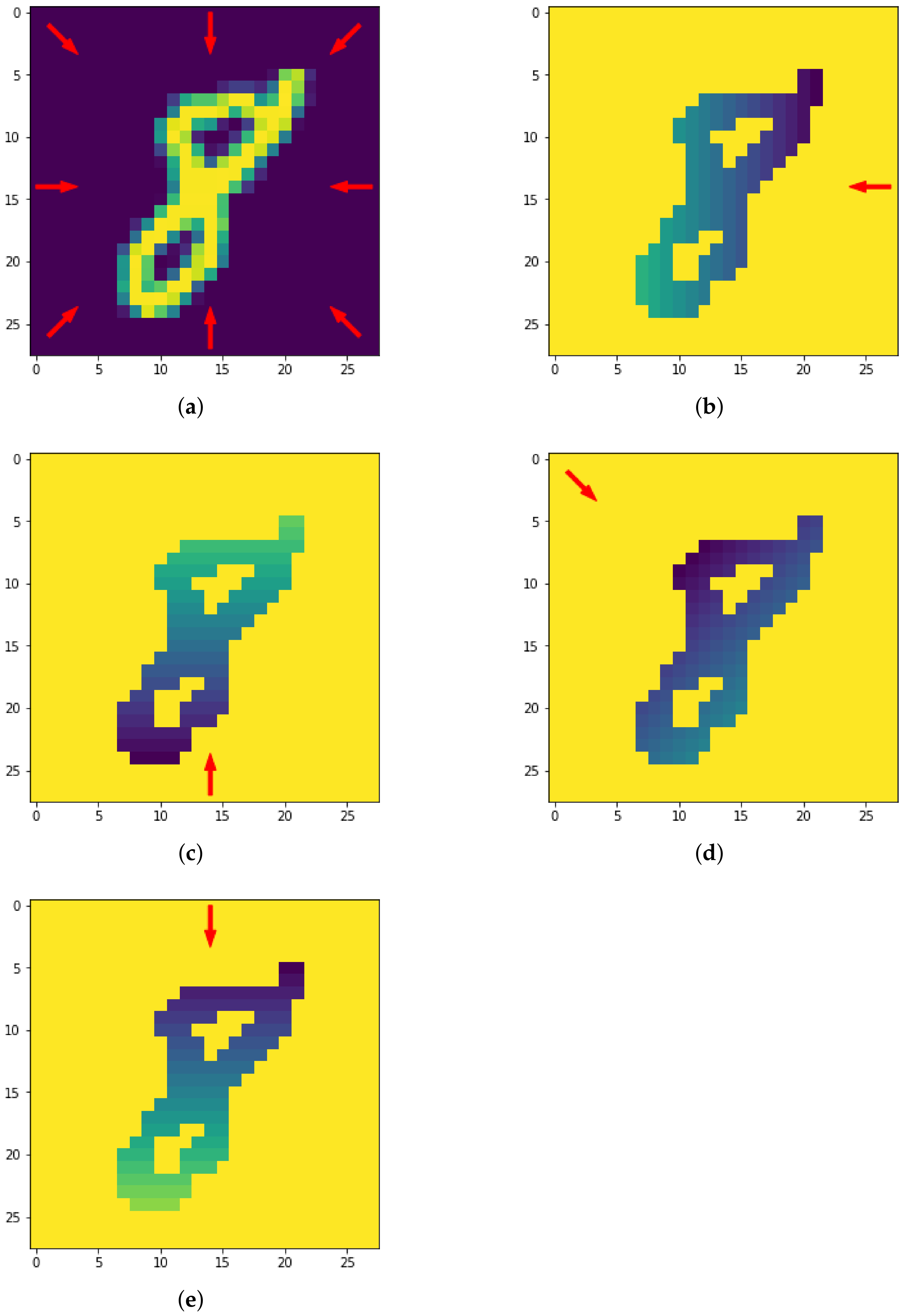
where and is the filtration value of the pixel farthest from v. We define eight different directions for the height filtration, namely the vectors , , , , , , , . In Figure 12, we show the different directions of filtration alongside four filtered images generated by the height filtration for different direction vectors. We highlight the fact that in Figure 11d and Figure 12a, for the digit “8”, one is the negative of the other for the reasons already mentioned.
4.2.2. Radial Filtration
Similarly to the height filtration, the radial filtration detects the emergence of topological features as we move away from a certain center of the image. This filtration is more suited to detect heterogeneity within the image, but it is way more context-dependent than the height filtration. In particular, the size of the image plays a crucial role in the choice of the centers. The radial filtration was introduced in [38,40]. Given a binary image and a center , the radial filtration of is defined as
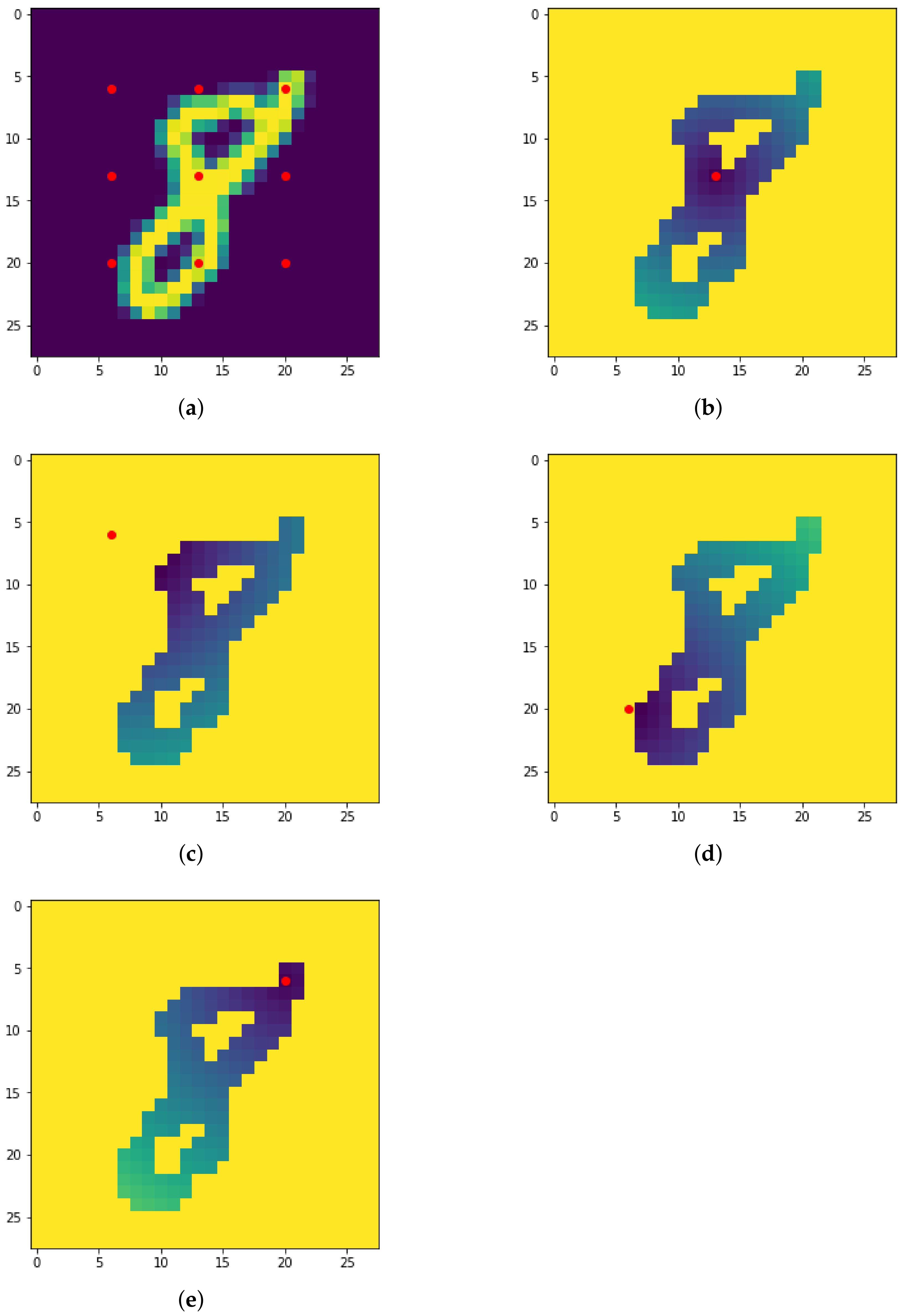
where and is the filtration value of the pixel farthest from c. We define nine centers for the radial filtration, namely the points , , , , , , , , . In Figure 13, we show the different centers of filtration alongside four filtered images generated by the radial filtration for different centers.
4.2.3. Density Filtration
Finally, the density filtration [38] measures the number of lighted pixels in the neighbors of a certain pixel and is better suited to detect clusters of lighted pixels. Given a binary image and a radius , the density filtration is defined as
where and is any norm. In our pipeline, we chose and the Euclidean norm. In Figure 14, we show an image from the MNIST dataset and the filtered image with respect to the density filtration with and the Euclidean norm.
4.2.4. Improved Pipeline
We have defined eight directions for the height filtration, nine centers for the radial filtration and one radius for the density filtration. The result is that from a single image, we now obtain 18 different PDs for each homology dimension, each corresponding to a different filtration/parameter combination. Similarly to how we handled the different homology dimensions, we follow two approaches. The first approach is to simply collapse all the PDs into one and then apply the pipeline from the PDs representation onwards. We refer to this approach as the ‘collapse approach’. The second idea is to first represent each one of the PDs with a vectorization method, concatenate the 18 vectors thus resulting and use this ‘multivector’ to classify the images. We refer to this approach as the ‘multivector approach’. We stress that the multivector approach and the collapse approach both result in two vectors, but the dimension of these vectors is very different. More precisely, the result of the multivector approach is 18 times the dimension of the collapse approach. There are of course major consequences in the computational cost of the two approaches, but as this is not the purpose of our study, we will overlook these aspects. In Table 4, we report the results of the collapse approach and in Table 5, we report the results of the multivector approach. Both the approaches are very satisfactory and represent a great improvement over the grayscale filtration. We can however notice how the representation methods are not as consistent as we would like. Table 6 reports the best single method for the MNIST dataset, and the accuracy results are very high. This means that the non-consistency of the representation is only due to the high accuracy of every representation method and not to a variability of the correct vectorization, thereby making the non-consistency less impactful.
4.2.5. Comparison with Other TDA Approaches
Finally, a comparison is made with two papers that also use TDA and the MNIST dataset. Our improved approach is partially inspired by the work of [38], in which the authors perform 26 filtrations of the same image. They compute 14 metrics for each of these filtrations, and the resulting vector of topological features for each image has a dimension of 728 (26 filtrations metrics homology dimensions). After a feature selection using the Pearson correlation index, only 84 not fully correlated features remain. The resulting vector is then passed to a random forest classifier. For the sake of comparison, since in our work we train only on a 5000 images subsample of the MNIST dataset with multiple classifiers, we repeat their experiment in our context. For this reason, the results reported in this section slightly differ from those obtained in the original work. In [41], the authors perform the height filtration along the horizontal and vertical axes, for each homology dimension, for a total of 8 PDs. They use some vectorization methods as well as kernel methods for PDs and an adaptive template system and then classify with the same classifiers as in our work (with the exclusion of lasso). Again, for the sake of comparison, we repeat the experiment in our context, only without the kernel method, for computational and comparison reasons. The results of both [38,41] are presented in Table 7. Regarding the results obtained by [41], with (TF), we indicate that the best method was tent functions. The results obtained from our improved pipeline are in line with, if not slightly better than, those obtained from other works. It should be noted that the pipeline described in [38] does not use representation methods but only metrics on Persistence Diagrams.
4.3. Fmnist
Fashion MNIST (FMNIST) is a dataset of Zalando’s article images, consisting of pixel grayscale images divided into ten classes, exactly like MNIST. FMNIST is intended to be a direct drop-in replacement for the original MNIST. This dataset is strongly adequate for our study, since we know that the topology of handwritten digits is almost always trivial, while this is not the case in fashion objects. For more information on the FMNIST dataset, we refer the reader to [42]. Figure 15 shows sample images from the FMNIST dataset. Since the context is fairly identical to Section 4.2, we follow exactly the same approach. Table 8 gives the results of the pipeline to the FMNIST dataset. Again, the results are not at all adequate, although there is a consistency in the vectorization method. Nevertheless, we can already observe a clear increase compared to the respective MNIST results (Table 3). This is in accordance with the fact that grayscale filtration is more suitable when the homology of the image is non-trivial, as in the case of fashion images. Following the approach used in the previous section, we introduce the exact same improvements to the pipeline as the context is precisely the same. In Figure 16, we show some filtered images for the FMNIST dataset. Table 9 and Table 10 report the results of, respectively, the collapse approach and the multivector approach for the FMNIST dataset. Both these approaches are a great improvement over the original pipeline, meaning that also for more complex images, a diversification of the filtration may be well suited. The dataset is clearly more convoluted than the MNIST dataset, and this may explain the significant drop in results compared to the previous section. The consistency of the representation is however very remarkable. Following Section 4.2.5, we compare our results with those obtained by the [38,41] pipelines. We highlight the fact that in both papers, the FMNIST dataset was not treated, but given the similarity of the two databases, we simply reused their code for MNIST. The results of both pipelines are reported in Table 11. Table 12 reports the best single method for the FMNIST dataset. The accuracy results for this application are quite surprising. In particular, our pipeline does not perform very well despite the improvement from the previous section. The pipeline from [38] achieves slightly better results, while the [41] pipeline performs best of all. Possible reasons may be a different choice of parameters but also a simpler filtration which, in this particular setting, is more suited for the dataset.
4.4. Collab
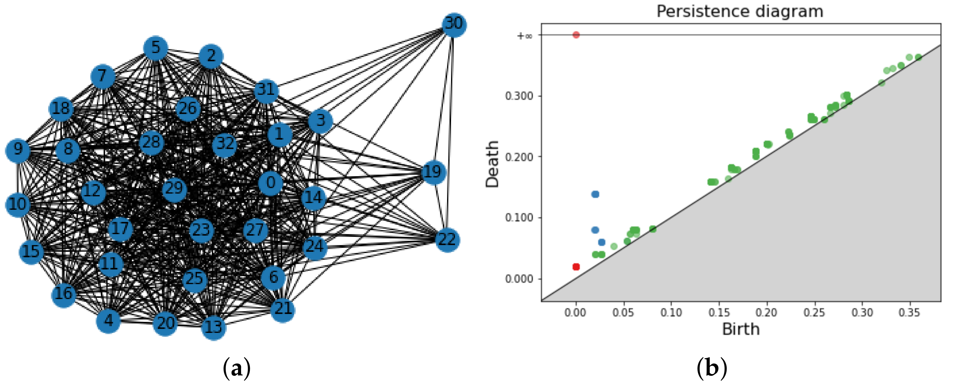
The COLLAB dataset is a network graphs dataset of scientific collaborations coming from [43]. It consists of 5000 graphs derived from three public collaboration datasets which also serve as labels: high energy physics, condensed matter physics and astro physics. Each node of the graphs is an author, and there is a link between two authors if they coauthor a scientific article. COLLAB is a dataset of weighted, undirected graphs. Every collaboration between n authors contributes to the edge weight between those authors of a factor . The vertices are not weighted; this means that all vertices immediately enter the filtration as 0-simplexes. The filtration value of the 1-simplexes is the weight of the edge connecting the two vertices, and for 2-simplexes, we chose as the filtration value the maximum weight of the edges forming it. For computational reasons, the maximum homology dimension computed is . In Figure 17, we show a graph of COLLAB and the associated PD. For aesthetic reasons, we have included only a small portion of the 2-simplexes, and the edge weight is not displayed. The graphs of this dataset are extremely connected, and the computational cost in order to compute their PD is very high. In Table 13, we report the results achieved by the pipeline on COLLAB dataset, and in Table 14, the best combination representation is the classifier. These results are quite satisfactory and in line with other topology-based methods, such as PersLay [44], achieving an accuracy of (mean accuracy over ten runs of a 10-fold classification evaluation).
5. Discussion
The proposed pipeline proved to be a valuable classification tool in various contexts. Moreover, some patterns emerged in the course of the experiments. In particular, for point clouds and graphs, it seems that the maximum homology dimension alone is sufficient to obtain very appreciable results. For images, on the other hand, only achieves good results. The ‘fused’ and ‘concat’ approaches are consistently among the best performers with the exception of the dynamic dataset where ‘fused’ fails. This discrepancy does not seem to be explained by heterogeneity in the number of points in the homology dimensions, which are comparable in all datasets with the exception of COLLAB. For these reasons, it would seem that regardless of the type of data under consideration and the number of points in the different homology dimensions, the ‘concat’ approach is the safest method. Alternatively, if the data are not images and one wishes to reduce the computational cost, using only the maximum homology dimension seems to be a viable option. No correlation emerged between data type and vectorization method. In general, it seems that Persistence Image and Persistence Landscape are always the safest options. In order to support these statements, an analysis of the statistical significance has been performed (using the paired t-test) on a subset of the results presented in Section 4. In the following, Table 15, Table 16, Table 17, Table 18 and Table 19 show the p-values associated with the mean accuracy results of the different vectorization methods for each homology dimension. For the sake of brevity, we describe in detail only Table 15. Table 15 has been computed as follows. In Section 4, we have computed the mean accuracy of each classifier and each vectorization method previously described over the course of the ten runs of the cross-validation. This consists of a matrix of 9 rows (one for each classifier) and 21 columns (one for each vectorization method). We have selected the best row (in terms of mean accuracy) for each vectorization method and tested each vectorization method against each other using the t-test function from scipy. For more information on the t-test and scipy, we refer the reader to [45,46]. In Section 4, we have assessed that PI is the best vectorization method for and ‘fused’, while PL is the best method for and ‘concat’. Table 15 ensures that these statements have statistical validity, because the p-value associated with these methods and homology dimensions is sufficiently small. In Table 19, we have followed the same procedure with the difference that we have compared each homological dimension against each other for every dataset. In particular, the p-value of the ‘concat’ approach is consistently small, confirming that its usefulness is supported by statistical results.
6. Conclusions
Results of classification discussed in the previous sections show that the proposed pipeline is a procedure able to maximize the capabilities of topological data analysis and Machine Learning. Such pipeline allows the analysis of digital data without restrictions such as data type or acquisition method. Moreover, the pipeline is not limited to the size of the dataset, which is often the case of the most recent and best-performing methods for classification based on deep learning architectures. In addition, interesting correlations arose between homology dimension and classification results. The concatenation of PDs in the different homology dimensions consistently seems to be the most suitable choice. In the very near future, we will further investigate the correlation between filtration, vectorization and data type in very challenging settings arising from real-world datasets, e.g., remote sensing (for climate prediction), and in Raman spectroscopy (for cancer staging).
Author Contributions
Conceptualization, F.C., D.M. and M.A.P.; Data curation, F.C.; Investigation, F.C.; Methodology, F.C., D.M. and M.A.P.; Software, F.C.; Supervision, D.M. and M.A.P.; Writing—original draft, F.C.; Writing—review and editing, F.C., D.M. and M.A.P. All authors have read and agreed to the published version of the manuscript.
Funding
This research received no external funding.
Conflicts of Interest
The authors declare no conflict of interest.
References
- Bronstein, M.M.; Bruna, J.; LeCun, Y.; Szlam, A.; Vandergheynst, P. Geometric deep learning: Going beyond euclidean data. IEEE Signal Process. Mag. 2017, 34, 18–42. [Google Scholar] [CrossRef]
- Monti, F.; Boscaini, D.; Masci, J.; Rodola, E.; Svoboda, J.; Bronstein, M.M. Geometric deep learning on graphs and manifolds using mixture model cnns. In Proceedings of the IEEE Conference on Computer Vision and Pattern Recognition, Honolulu, HI, USA, 21–26 July 2017; pp. 5115–5124. [Google Scholar]
- Krizhevsky, A.; Sutskever, I.; Hinton, G.E. Imagenet classification with deep convolutional neural networks. Adv. Neural Inf. Process. Syst. 2012, 25. Available online: https://proceedings.neurips.cc/paper/2012/file/c399862d3b9d6b76c8436e924a68c45b-Paper.pdf (accessed on 1 February 2022). [CrossRef]
- Bergomi, M.G.; Frosini, P.; Giorgi, D.; Quercioli, N. Towards a topological–geometrical theory of group equivariant non-expansive operators for data analysis and machine learning. Nat. Mach. Intell. 2019, 1, 423–433. [Google Scholar] [CrossRef]
- Conti, F.; Frosini, P.; Quercioli, N. On the Construction of Group Equivariant Non-Expansive Operators via Permutants and Symmetric Functions. Front. Artif. Intell. 2022, 5, 786091. [Google Scholar] [CrossRef] [PubMed]
- Carlsson, G. Topology and data. Bull. Am. Math. Soc. 2009, 46, 255–308. [Google Scholar] [CrossRef]
- Lum, P.; Singh, G.; Lehman, A.; Ishkanov, T.; Vejdemo-Johansson, M.; Alagappan, M.; Carlsson, J.; Carlsson, G. Extracting insights from the shape of complex data using topology. Sci. Rep. 2013, 3, 1236. [Google Scholar] [CrossRef]
- Tauzin, G.; Lupo, U.; Tunstall, L.; Pérez, J.B.; Caorsi, M.; Medina-Mardones, A.M.; Dassatti, A.; Hess, K. giotto-tda: A Topological Data Analysis Toolkit for Machine Learning and Data Exploration. J. Mach. Learn. Res. 2021, 22, 1–6. [Google Scholar]
- Nielson, J.L.; Paquette, J.; Liu, A.W.; Guandique, C.F.; Tovar, C.A.; Inoue, T.; Irvine, K.A.; Gensel, J.C.; Kloke, J.; Petrossian, T.C.; et al. Topological data analysis for discovery in preclinical spinal cord injury and traumatic brain injury. Nat. Commun. 2015, 6, 1–12. [Google Scholar]
- Chazal, F.; Fasy, B.T.; Lecci, F.; Rinaldo, A.; Wasserman, L. Stochastic convergence of persistence landscapes and silhouettes. In Proceedings of the Thirtieth Annual Symposium on Computational Geometry, Kyoto, Japan, 8–11 June 2014; pp. 474–483. [Google Scholar]
- Bubenik, P. Statistical topological data analysis using persistence landscapes. J. Mach. Learn. Res. 2015, 16, 77–102. [Google Scholar]
- Umeda, Y. Time series classification via topological data analysis. Inf. Media Technol. 2017, 12, 228–239. [Google Scholar] [CrossRef]
- Adams, H.; Emerson, T.; Kirby, M.; Neville, R.; Peterson, C.; Shipman, P.; Chepushtanova, S.; Hanson, E.; Motta, F.; Ziegelmeier, L. Persistence images: A stable vector representation of persistent homology. J. Mach. Learn. Res. 2017, 18, 1–35. [Google Scholar]
- Chen, C.; Ni, X.; Bai, Q.; Wang, Y. A topological regularizer for classifiers via persistent homology. In Proceedings of the 22nd International Conference on Artificial Intelligence and Statistics, Naha, Japan, 16–18 April 2019; pp. 2573–2582. [Google Scholar]
- Pun, C.S.; Xia, K.; Lee, S.X. Persistent-Homology-based Machine Learning and its Applications—A Survey. arXiv 2018, arXiv:1811.00252. [Google Scholar] [CrossRef]
- Corbet, R.; Fugacci, U.; Kerber, M.; Landi, C.; Wang, B. A kernel for multi-parameter persistent homology. Comput. Graph. X 2019, 2, 100005. [Google Scholar] [CrossRef] [PubMed]
- Hatcher, A. Algebraic Topology; Cambridge University Press: Cambridge, UK, 2002; p. xii+544. [Google Scholar]
- Verri, A.; Uras, C.; Frosini, P.; Ferri, M. On the use of size functions for shape analysis. Biol. Cybern. 1993, 70, 99–107. [Google Scholar] [CrossRef]
- Epstein, C.L.; Carlsson, G.E.; Edelsbrunner, H. Topological data analysis. Inverse Probl. 2011, 27, 120201. [Google Scholar]
- Carlsson, G.; Zomorodian, A.; Collins, A.; Guibas, L. Persistence Barcodes for Shapes. In Proceedings of the 2004 Eurographics/ACM SIGGRAPH Symposium on Geometry Processing, Nice, France, 8–10 July 2004; Association for Computing Machinery: New York, NY, USA, 2004; pp. 124–135. [Google Scholar] [CrossRef]
- Frosini, P. A distance for similarity classes of submanifolds of a Euclidean space. Bull. Aust. Math. Soc. 1990, 42, 407–415. [Google Scholar] [CrossRef]
- Biasotti, S.; Cerri, A.; Frosini, P.; Giorgi, D.; Landi, C. Multidimensional size functions for shape comparison. J. Math. Imaging Vis. 2008, 32, 161–179. [Google Scholar] [CrossRef]
- Akkiraju, N.; Edelsbrunner, H.; Facello, M.; Fu, P.; Mucke, E.; Varela, C. Alpha shapes: Definition and software. In Proceedings of the 1st International Computational Geometry Software Workshop, Minneapolis, MN, USA, 1995; Volume 63, p. 66. [Google Scholar]
- Kaczynski, T.; Mischaikow, K.M.; Mrozek, M. Computational Homology; Springer: Berlin/Heidelberg, Germany, 2004; Volume 3. [Google Scholar]
- Biasotti, S.; De Floriani, L.; Falcidieno, B.; Frosini, P.; Giorgi, D.; Landi, C.; Papaleo, L.; Spagnuolo, M. Describing shapes by geometrical-topological properties of real functions. ACM Comput. Surv. (CSUR) 2008, 40, 1–87. [Google Scholar] [CrossRef]
- Carlsson, G.; Zomorodian, A. The theory of multidimensional persistence. Discret. Comput. Geom. 2009, 42, 71–93. [Google Scholar] [CrossRef]
- Edelsbrunner, H.; Harer, J. Persistent homology-a survey. Contemp. Math. 2008, 453, 257–282. [Google Scholar]
- Cohen-Steiner, D.; Edelsbrunner, H.; Harer, J. Stability of persistence diagrams. Discret. Comput. Geom. 2007, 37, 103–120. [Google Scholar] [CrossRef]
- The GUDHI Project. GUDHI User and Reference Manual, 3.5.0 ed.; GUDHI Editorial Board; 2022; Available online: https://gudhi.inria.fr/doc/3.5.0/ (accessed on 1 May 2022).
- Cortes, C.; Vapnik, V. Support-vector networks. Mach. Learn. 1995, 20, 273–297. [Google Scholar] [CrossRef]
- Breiman, L. Random forests. Mach. Learn. 2001, 45, 5–32. [Google Scholar] [CrossRef]
- Hoerl, A.E.; Kennard, R.W. Ridge regression: Biased estimation for nonorthogonal problems. Technometrics 1970, 12, 55–67. [Google Scholar] [CrossRef]
- Tibshirani, R. Regression shrinkage and selection via the lasso. J. R. Stat. Soc. Ser. (Methodol.) 1996, 58, 267–288. [Google Scholar] [CrossRef]
- Pedregosa, F.; Varoquaux, G.; Gramfort, A.; Michel, V.; Thirion, B.; Grisel, O.; Blondel, M.; Prettenhofer, P.; Weiss, R.; Dubourg, V.; et al. Scikit-learn: Machine Learning in Python. J. Mach. Learn. Res. 2011, 12, 2825–2830. [Google Scholar]
- Allen, D.M. The Relationship Between Variable Selection and Data Agumentation and a Method for Prediction. Technometrics 1974, 16, 125–127. Available online: http://xxx.lanl.gov/abs/https://www.tandfonline.com/doi/pdf/10.1080/00401706.1974.10489157 (accessed on 1 November 2021). [CrossRef]
- Chung, Y.M.; Lawson, A. Persistence Curves: A Canonical Framework for Summarizing Persistence Diagrams. 2021. Available online: http://xxx.lanl.gov/abs/1904.07768 (accessed on 1 February 2022).
- Deng, L. The mnist database of handwritten digit images for machine learning research. IEEE Signal Process. Mag. 2012, 29, 141–142. [Google Scholar] [CrossRef]
- Garin, A.; Tauzin, G. A Topological “Reading” Lesson: Classification of MNIST using TDA. In Proceedings of the 2019 18th IEEE International Conference On Machine Learning And Applications (ICMLA), Boca Raton, FL, USA, 16–19 December 2019; pp. 1551–1556. [Google Scholar] [CrossRef]
- Turner, K.; Mukherjee, S.; Boyer, D.M. Persistent Homology Transform for Modeling Shapes and Surfaces. 2014. Available online: http://arxiv.org/abs/1310.1030 (accessed on 1 February 2022).
- Lida, K.; Dłotko, P.; Scolamiero, M.; Levi, R.; Shillcock, J.; Hess, K.; Markram, H. A Topological Representation of Branching Neuronal Morphologies. Neuroinformatics 2018, 16, 3–13. [Google Scholar] [CrossRef]
- Barnes, D.; Polanco, L.; Perea, J.A. A Comparative Study of Machine Learning Methods for Persistence Diagrams. Front. Artif. Intell. 2021, 4, 681174. [Google Scholar] [CrossRef]
- Xiao, H.; Rasul, K.; Vollgraf, R. Fashion-MNIST: A Novel Image Dataset for Benchmarking Machine Learning Algorithms. 2017. Available online: http://arxiv.org/abs/1708.07747 (accessed on 1 February 2022).
- Yanardag, P.; Vishwanathan, S. Deep Graph Kernels. In Proceedings of the 21th ACM SIGKDD International Conference on Knowledge Discovery and Data Mining, Sydney, Australia, 10–13 August 2015; Association for Computing Machinery: New York, NY, USA, 2015; pp. 1365–1374. [Google Scholar] [CrossRef]
- Carrière, M.; Chazal, F.; Ike, Y.; Lacombe, T.; Royer, M.; Umeda, Y. PersLay: A Neural Network Layer for Persistence Diagrams and New Graph Topological Signatures. In Proceedings of the 23rd International Conference on Artificial Intelligence and Statistics, AISTATS 2020, Palermo, Italy, 26–28 August 2020; Volume 108, pp. 2786–2796. [Google Scholar]
- Kim, T.K. T test as a parametric statistic. Korean J. Anesthesiol. 2015, 68, 540–546. [Google Scholar] [CrossRef] [PubMed]
- Virtanen, P.; Gommers, R.; Oliphant, T.E.; Haberland, M.; Reddy, T.; Cournapeau, D.; Burovski, E.; Peterson, P.; Weckesser, W.; Bright, J.; et al. SciPy 1.0: Fundamental Algorithms for Scientific Computing in Python. Nat. Methods 2020, 17, 261–272. [Google Scholar] [CrossRef] [PubMed] [Green Version]
Figure 1.
The sphere (a) bounds a 2-dimensional void. The torus (b) bounds a 2-dimensional void and two 1-dimensional holes. Images: Geek3 and YassinMrabet via Wikipedia.
Figure 1.
The sphere (a) bounds a 2-dimensional void. The torus (b) bounds a 2-dimensional void and two 1-dimensional holes. Images: Geek3 and YassinMrabet via Wikipedia.

Figure 2.
The pipeline for a topological study of digital data in a Machine Learning context. A filtration associates a persistence diagram to the digital data. The persistence diagram is then vectorized by means of various vectorization methods. Finally, the vector is fed to a Machine Learning classifier.

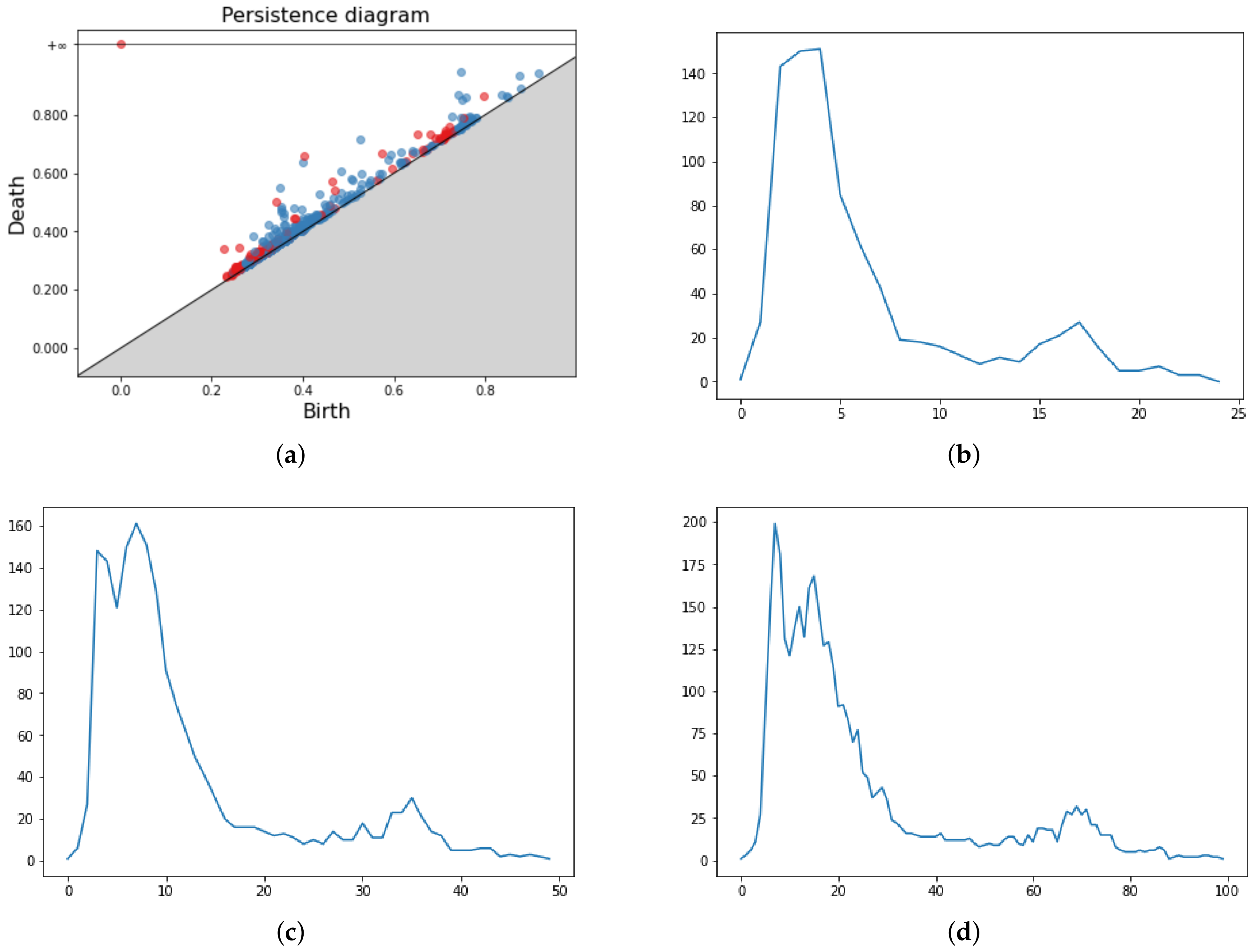
Figure 3.
Pipeline application for point cloud data (a). The persistence diagram associated (b). In the second and third rows, four different vectorization methods for the same PD, namely Persistence Images (c), Persistence Landscapes (d), Persistence Silhouette (e) and Betti Curves (f).
Figure 3.
Pipeline application for point cloud data (a). The persistence diagram associated (b). In the second and third rows, four different vectorization methods for the same PD, namely Persistence Images (c), Persistence Landscapes (d), Persistence Silhouette (e) and Betti Curves (f).

Figure 4.
Pixel connection in cubical complexes.

Figure 5.
Persistence Diagram (a) and three Persistence Images for respectively in (b–d).

Figure 6.
Persistence Diagram (a) and three Persistence Landscapes for respectively in (b–d).


Figure 7.
Persistence Diagram (a) and three Persistence Silhouettes for and , respectively in (b–d).
Figure 7.
Persistence Diagram (a) and three Persistence Silhouettes for and , respectively in (b–d).


Figure 8.
Persistence Diagram (a) and three Betti curves for and , respectively, in (b–d).

Figure 9.
Example of truncated orbits for the first 1000 iterations of the linked twisted map for different r. From (a) to (e) r is, respectively, and .
Figure 9.
Example of truncated orbits for the first 1000 iterations of the linked twisted map for different r. From (a) to (e) r is, respectively, and .

Figure 10.
Example of truncated orbits for the first 1000 iterations of the linked twisted map for and five different starting points (a–e).
Figure 10.
Example of truncated orbits for the first 1000 iterations of the linked twisted map for and five different starting points (a–e).

Figure 11.
Sample images from MNIST dataset. It can be seen at a glance that the homology of different digits is almost always trivial (for (b,c)) or close to trivial (for (a,d,e)).
Figure 11.
Sample images from MNIST dataset. It can be seen at a glance that the homology of different digits is almost always trivial (for (b,c)) or close to trivial (for (a,d,e)).

Figure 12.
The eight directions used for the height filtration (a) and resulting filtrated images along four directions (b–e).
Figure 12.
The eight directions used for the height filtration (a) and resulting filtrated images along four directions (b–e).

Figure 13.
The nine centers used for the radial filtration (a) and resulting filtrated images with respect to four different centers (b–e).
Figure 13.
The nine centers used for the radial filtration (a) and resulting filtrated images with respect to four different centers (b–e).

Figure 14.
The original digit “8” (a) and the resulting filtered image with respect to the density filtration with radius (b).
Figure 14.
The original digit “8” (a) and the resulting filtered image with respect to the density filtration with radius (b).

Figure 15.
(a–e) Sample images from FMNIST dataset. Classifying these images is clearly more difficult than with the MNIST dataset.
Figure 15.
(a–e) Sample images from FMNIST dataset. Classifying these images is clearly more difficult than with the MNIST dataset.

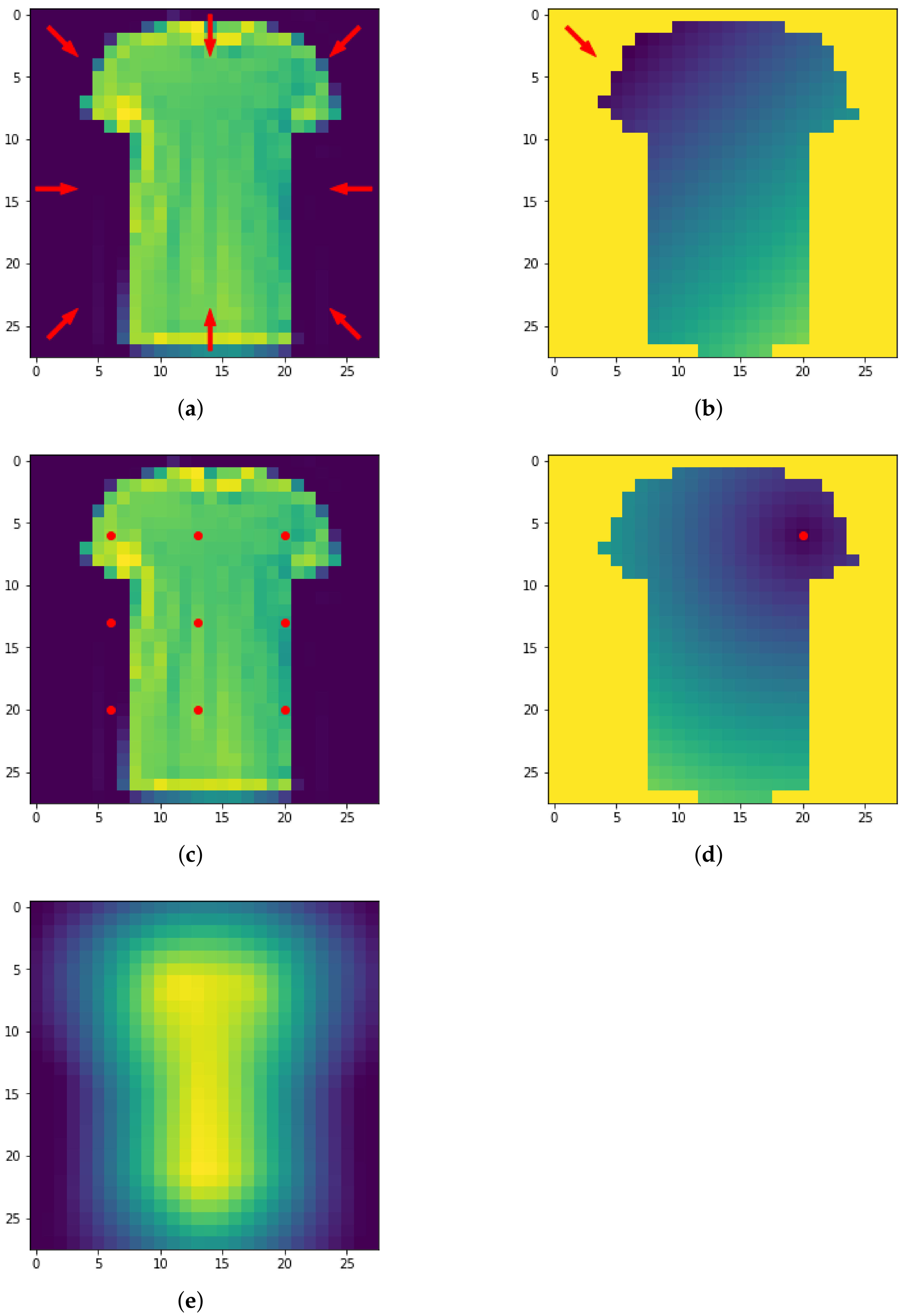
Figure 16.
The eight directions used for the height filtration (a) and resulting filtrated image (b). The nine centers used for the radial filtration (c,d). Density filtered image (e).
Figure 16.
The eight directions used for the height filtration (a) and resulting filtrated image (b). The nine centers used for the radial filtration (c,d). Density filtered image (e).

Figure 17.
A graph of COLLAB (a) and the corresponding PD (b). For aesthetic reasons, only a small sample of 2-simplexes are shown and the edge weight is not displayed. In figure (b) the PD in dimension 0–2 are visualized in the same plot: points are red for PD in dimension 0, blue for PD in dimension 1 and green for dimension 2.


Table 1.
Accuracy for the dynamical system dataset. (PI: persistent image; PL: persistent landscape; BC: Betti curve).
Table 1.
Accuracy for the dynamical system dataset. (PI: persistent image; PL: persistent landscape; BC: Betti curve).
| Accuracy | (Fused) | (Concat) | ||
|---|---|---|---|---|
| Run 1 | (PI) | (PL) | (PI) | (PL) |
| Run 2 | (PI) | (PL) | (PI) | (PL) |
| Run 3 | (PI) | (PL) | (PI) | (PL) |
| Run 4 | (PI) | (BC) | (PI) | (BC) |
| Run 5 | (PI) | (PL) | (PI) | (PL) |
| Run 6 | (PI) | (PL) | (PI) | (PL) |
| Run 7 | (PI) | (PL) | (PI) | (PL) |
| Run 8 | (PI) | (PL) | (PI) | (PL) |
| Run 9 | (PI) | (PL) | (PI) | (BC) |
| Run 10 | (PI) | (PL) | (PI) | (PL) |
| Mean: |
Table 2.
Best method for the dynamical system dataset.
| Homology | Accuracy | Vectorization | Classifier |
|---|---|---|---|
| Persistence Images | RandomForestClassifier | ||
| Persistence Landscapes | SVC(kernel = ‘rbf’, C = 10) | ||
| (fused) | Persistence Images | RandomForestClassifier | |
| (concat) | Persistence Landscapes | RandomForestClassifier |
Table 3.
Accuracy for MNIST dataset. (PI: persistent image; PL: persistent landscape; PS: persistent silhouette; BC: Betti curve).
Table 3.
Accuracy for MNIST dataset. (PI: persistent image; PL: persistent landscape; PS: persistent silhouette; BC: Betti curve).
| Accuracy | (Fused) | (Concat) | ||
|---|---|---|---|---|
| Run 1 | (PI) | (PL) | (PI) | (PL) |
| Run 2 | (PI) | (PL) | (PI) | (PL) |
| Run 3 | (PI) | (PL) | (PI) | (PS) |
| Run 4 | (PI) | (PL) | (PI) | (PL) |
| Run 5 | (PS) | (PL) | (PI) | (PL) |
| Run 6 | (PI) | (PL) | (PI) | (PL) |
| Run 7 | (PI) | (PL) | (PI) | (PL) |
| Run 8 | (PS) | (PL) | (PI) | (PL) |
| Run 9 | (PI) | (PL) | (PI) | (BC) |
| Run 10 | (PI) | (PL) | (PI) | (PL) |
| Mean: |
Table 4.
Accuracy for MNIST dataset of the collapse approach. (PI: persistent image; PL: persistent landscape).
Table 4.
Accuracy for MNIST dataset of the collapse approach. (PI: persistent image; PL: persistent landscape).
| Accuracy | (Fused) | (Concat) | ||
|---|---|---|---|---|
| Run 1 | (PI) | (PL) | (PI) | (PI) |
| Run 2 | (PI) | (PI) | (PI) | (PI) |
| Run 3 | (PI) | (PI) | (PI) | (PI) |
| Run 4 | (PI) | (PL) | (PI) | (PI) |
| Run 5 | (PI) | (PI) | (PI) | (PI) |
| Run 6 | (PL) | (PL) | (PI) | (PI) |
| Run 7 | (PI) | (PL) | (PI) | (PL) |
| Run 8 | (PI) | (PL) | (PI) | (PI) |
| Run 9 | (PL) | (PL) | (PI) | (PI) |
| Run 10 | (PI) | (PI) | (PI) | (PL) |
| Mean: |
Table 5.
Accuracy for MNIST dataset of the multivector approach. (PI: persistent image; PL: persistent landscape; PS: persistent silhouette; BC: Betti curve).
Table 5.
Accuracy for MNIST dataset of the multivector approach. (PI: persistent image; PL: persistent landscape; PS: persistent silhouette; BC: Betti curve).
| Accuracy | (Fused) | (Concat) | ||
|---|---|---|---|---|
| Run 1 | (PL) | (PL) | (PI) | (PL) |
| Run 2 | (PL) | (PL) | (BC) | (PL) |
| Run 3 | (PL) | (PS) | (BC) | (PL) |
| Run 4 | (PL) | (PL) | (BC) | (PS) |
| Run 5 | (PL) | (PL) | (BC) | (PL) |
| Run 6 | (PL) | (PL) | (BC) | (PL) |
| Run 7 | (PL) | (PL) | (PI) | (PL) |
| Run 8 | (PL) | (PL) | (BC) | (PS) |
| Run 9 | (PL) | (PL) | (PL) | (PL) |
| Run 10 | (PL) | (PL) | (BC) | (PL) |
| Mean: |
Table 6.
Best method for MNIST dataset.
| Homology | Accuracy | Vectorization | Classifier | Approach |
|---|---|---|---|---|
| PI | SVC(kernel = ‘rbf’, C = 10) | Multivector | ||
| PL | SVC(kernel = ‘rbf’, C = 20) | Collapse | ||
| (fused) | PI | SVC(kernel = ‘rbf’, C = 20) | Multivector | |
| (concat) | PI | SVC(kernel = ‘rbf’, C = 20) | Multivector |
Table 7.
Accuracy for MNIST dataset of [38] pipeline and [41] pipeline. (TF: tent function; PI: persistent image).
| Accuracy | [38] Pipeline | [41] Pipeline |
|---|---|---|
| Run 1 | (TF) | |
| Run 2 | (TF) | |
| Run 3 | (TF) | |
| Run 4 | (PI) | |
| Run 5 | (TF) | |
| Run 6 | (TF) | |
| Run 7 | (TF) | |
| Run 8 | (PI) | |
| Run 9 | (TF) | |
| Run 10 | (TF) | |
| Mean: |
Table 8.
Accuracy for FMNIST dataset. (PI: persistent image).
| Accuracy | (Fused) | (Concat) | ||
|---|---|---|---|---|
| Run 1 | (PI) | (PI) | (PI) | (PI) |
| Run 2 | (PI) | (PI) | (PI) | (PI) |
| Run 3 | (PI) | (PI) | (PI) | (PI) |
| Run 4 | (PI) | (PI) | (PI) | (PI) |
| Run 5 | (PI) | (PI) | (PI) | (PI) |
| Run 6 | (PI) | (PI) | (PI) | (PI) |
| Run 7 | (PI) | (PI) | (PI) | (PI) |
| Run 8 | (PI) | (PI) | (PI) | (PI) |
| Run 9 | (PI) | (PI) | (PI) | (PI) |
| Run 10 | (PI) | (PI) | (PI) | (PI) |
| Mean: |
Table 9.
Accuracy for FMNIST dataset of the collapse approach. (PI: persistent image; PL: persistent landscape).
Table 9.
Accuracy for FMNIST dataset of the collapse approach. (PI: persistent image; PL: persistent landscape).
| Accuracy | (Fused) | (Concat) | ||
|---|---|---|---|---|
| Run 1 | (PL) | (PI) | (PL) | (PL) |
| Run 2 | (PL) | (PI) | (PL) | (PL) |
| Run 3 | (PL) | (PI) | (PL) | (PL) |
| Run 4 | (PL) | (PL) | (PL) | (PL) |
| Run 5 | (PL) | (PI) | (PL) | (PL) |
| Run 6 | (PL) | (PI) | (PL) | (PL) |
| Run 7 | (PL) | (PI) | (PL) | (PL) |
| Run 8 | (PL) | (PI) | (PL) | (PL) |
| Run 9 | (PL) | (PL) | (PI) | (PL) |
| Run 10 | (PL) | (PL) | (PL) | (PL) |
| Mean: |
Table 10.
Accuracy for FMNIST dataset of the multivector approach. (PL: persistent landscape; PS: persistent silhouette).
Table 10.
Accuracy for FMNIST dataset of the multivector approach. (PL: persistent landscape; PS: persistent silhouette).
| Accuracy | (Fused) | (Concat) | ||
|---|---|---|---|---|
| Run 1 | (PL) | (PL) | (PL) | (PL) |
| Run 2 | (PL) | (PS) | (PL) | (PL) |
| Run 3 | (PL) | (PL) | (PL) | (PL) |
| Run 4 | (PL) | (PL) | (PL) | (PL) |
| Run 5 | (PL) | (PL) | (PL) | (PL) |
| Run 6 | (PL) | (PL) | (PL) | (PL) |
| Run 7 | (PL) | (PL) | (PL) | (PL) |
| Run 8 | (PL) | (PL) | (PL) | (PL) |
| Run 9 | (PL) | (PL) | (PL) | (PL) |
| Run 10 | (PL) | (PL) | (PL) | (PL) |
| Mean: |
Table 11.
Accuracy for FMNIST dataset of [38] pipeline and [41] pipeline. (PI: persistent image; TF: tent function).
| Accuracy | [38] Pipeline | [41] Pipeline |
|---|---|---|
| Run 1 | (PI) | |
| Run 2 | (PI) | |
| Run 3 | (TF) | |
| Run 4 | (PI) | |
| Run 5 | (PI) | |
| Run 6 | (PI) | |
| Run 7 | (PI) | |
| Run 8 | (PI) | |
| Run 9 | (PI) | |
| Run 10 | (PI) | |
| Mean: |
Table 12.
Best method for FMNIST dataset.
| Homology | Accuracy | Vectorization | Classifier | Approach |
|---|---|---|---|---|
| PL | RFC | Multivector | ||
| PI | RFC | Collapse | ||
| (fused) | PL | RFC | Multivector | |
| (concat) | PL | RFC | Multivector |
Table 13.
Accuracy for COLLAB dataset. (PI: persistent image; PL: persistent landscape; PS: persistent silhouette; BC: Betti curve).
Table 13.
Accuracy for COLLAB dataset. (PI: persistent image; PL: persistent landscape; PS: persistent silhouette; BC: Betti curve).
| Accuracy | (Fused) | (Concat) | |||
|---|---|---|---|---|---|
| Run 1 | (PI) | (PS) | (PI) | (PI) | (PI) |
| Run 2 | (PI) | (PS) | (PI) | (PI) | (PI) |
| Run 3 | (PI) | (PS) | (PI) | (PI) | (PI) |
| Run 4 | (BC) | (PL) | (PI) | (PI) | (PI) |
| Run 5 | (BC) | (PS) | (PI) | (PI) | (PI) |
| Run 6 | (PI) | (PS) | (PI) | (PI) | (PI) |
| Run 7 | (PI) | (PS) | (PI) | (PI) | (PI) |
| Run 8 | (BC) | (PS) | (PI) | (PI) | (PI) |
| Run 9 | (PS) | (PS) | (PI) | (PI) | (PI) |
| Run 10 | (PS) | (PS) | (PI) | (PI) | (PI) |
| Mean: |
Table 14.
Best method for COLLAB dataset.
| Homology | Accuracy | Vectorization | Classifier |
|---|---|---|---|
| Betti Curves | RandomForestClassifier | ||
| Persistence Silhouette | RandomForestClassifier | ||
| Persistence Images | RandomForestClassifier | ||
| (fused) | Persistence Images | RandomForestClassifier | |
| (concat) | Persistence Images | RandomForestClassifier |
Table 15.
p-value statistic for the dynamical system dataset.
| p-Value | Fused | Concat | ||
|---|---|---|---|---|
| PI vs. PL | 2.03 × | |||
| PI vs. PS | ||||
| PI vs. BC | ||||
| PL vs. PS | Null | |||
| PL vs. BC | Null | Null | ||
| PS vs. BC | Null |
Table 16.
p-value statistic for the MNIST dataset.
| p-Value | Fused | Concat | ||
|---|---|---|---|---|
| PI vs. PL | 4.55 × | |||
| PI vs. PS | ||||
| PI vs. BC | ||||
| PL vs. PS | ||||
| PL vs. BC | ||||
| PS vs. BC |
Table 17.
p-value statistic for the FMNIST dataset.
| p-Value | Fused | Concat | ||
|---|---|---|---|---|
| PI vs. PL | 2.02 × | |||
| PI vs. PS | ||||
| PI vs. BC | ||||
| PL vs. PS | ||||
| PL vs. BC | ||||
| PS vs. BC |
Table 18.
p-value statistic for the COLLAB dataset.
| p-Value | Fused | Concat | |||
|---|---|---|---|---|---|
| PI vs. PL | 3.73 × | ||||
| PI vs. PS | |||||
| PI vs. BC | |||||
| PL vs. PS | |||||
| PL vs. BC | |||||
| PS vs. BC |
Table 19.
p-value statistic for the homology dimensions.
| p-Value | Dynamical | MNIST | FMNIST | COLLAB |
|---|---|---|---|---|
| vs. | 5.71 × | |||
| vs. | - | - | - | |
| vs. fused | ||||
| vs. concat | ||||
| vs. | - | - | - | |
| vs. fused | ||||
| vs. concat | ||||
| vs. fused | - | - | - | |
| vs. concat | - | - | - | |
| fused vs. concat |
Publisher’s Note: MDPI stays neutral with regard to jurisdictional claims in published maps and institutional affiliations. |
© 2022 by the authors. Licensee MDPI, Basel, Switzerland. This article is an open access article distributed under the terms and conditions of the Creative Commons Attribution (CC BY) license (https://creativecommons.org/licenses/by/4.0/).
Share and Cite
MDPI and ACS Style
Conti, F.; Moroni, D.; Pascali, M.A. A Topological Machine Learning Pipeline for Classification. Mathematics 2022, 10, 3086. https://doi.org/10.3390/math10173086
AMA Style
Conti F, Moroni D, Pascali MA. A Topological Machine Learning Pipeline for Classification. Mathematics. 2022; 10(17):3086. https://doi.org/10.3390/math10173086
Chicago/Turabian StyleConti, Francesco, Davide Moroni, and Maria Antonietta Pascali. 2022. "A Topological Machine Learning Pipeline for Classification" Mathematics 10, no. 17: 3086. https://doi.org/10.3390/math10173086
Note that from the first issue of 2016, this journal uses article numbers instead of page numbers. See further details here.