Coherent Forecasting for a Mixed Integer-Valued Time Series Model

Abstract

In commerce, economics, engineering and the sciences, quantitative methods based on statistical models for forecasting are very useful tools for prediction and decision. There is an abundance of papers on forecasting for continuous-time series but relatively fewer papers for time series of counts which require special consideration due to the integer nature of the data. A popular method for modelling is the method of mixtures which is known for its flexibility and thus improved prediction capability. This paper studies the coherent forecasting for a flexible stationary mixture of Pegram and thinning (MPT) process, and develops the likelihood-based asymptotic distribution. Score functions and the Fisher information matrix are presented. Numerical studies are used to assess the performance of the forecasting methods. Also, a comparison is made with existing discrete-valued time series models. Finally, the practical application is illustrated with two sets of real data. It is shown that the mixture model provides good forecasting performance.

1. Introduction

Forecasting in Box–Jenkins models based on the conditional mean has been well established in time series modelling. However, the forecasting method in continuous-time series may not be applicable to handle integer-valued data as the conditional mean usually yields non-integer forecasts. In discrete-time series modelling, coherent forecasting replaces conventional forecasting to produce an integer forecast. Integer-valued time series data have appeared in many contexts, for example, compensation claims, crime data, unemployment count, and the number of cases of recent coronavirus outbreaks. Hence, coherent forecasting, especially those based on the conditional median and mode, is getting popular for integer forecasts. This tool is indispensable in commerce, economics, and the sciences as it provides insights in prediction and decision making. This paper presents the coherent forecasting for a mixture model, namely a mixture of Pegram and thinning (MPT) process as introduced by [1] Mixture models provide a flexible approach for modelling heterogeneity and multimodality in time series. There is much interest in this mixture approach for time series modelling. Ref. [2] considered this MPT(1) model with serially dependent innovation. By using this mixture of Pegram and binomial thinning operators, Ref. [3] examined a bounded INAR(1) model which caters for equi-, under- and over-dispersion. Recently, Ref. [4] examined a new bounded integer autoregressive process model also based on this mixture method.

The development of integer-valued time series models began three decades ago when [5] first introduced the discrete-time series models. Thereafter, generalizations and extensions, statistical inference and some other relevant investigations such as outlier detection have been extensively discussed. There is limited study on coherent forecasting for discrete time series. Ref. [6] considered four methods of coherent forecasting: k-step ahead conditional mean, median, mode and distribution. If a time series has low counts, point mass forecasting is employed where individual probabilities are assigned to the few possible outcomes that the forecast value may take. Later, Ref. [7] examined coherent forecasting issues related to the Poisson integer-valued autoregressive model of order one (INAR(1)) and [8] extended this to INAR(p). Using a Bayesian approach, Ref. [9] proposed a general method for producing coherent forecasts of low count data which are based upon the k-step–ahead predictive probability mass function. Ref. [10] considered the computer-intensive block-of-block bootstrap techniques for coherent forecasting. Ref. [11] developed the coherent forecasting in Binomial AR(p) model. Ref. [12] studied the coherent forecasting for zero-inflated Poisson fitted in INAR, specifically for the order-one process. More generally, Ref. [13] extended the discussion to include the stationary integer-valued ARMA models. Ref. [12] proposed the coherent forecasting for count data using Box–Jenkins’s AR(p) model. Ref. [14] discussed the forecast for geometric-type INAR(1) models. Recently, Ref. [15] investigated the forecast errors for the conditional linear autoregressive model. Due to the flexibility of the mixture MPT model to cater for heterogeneity and multimodality, and the practical importance of forecasting, we are motivated to examine the performance of the MPT model in coherent forecasting.

The paper is arranged as follows. Section 2 provides a brief background for discrete-time series models which serves as the framework for the models to be discussed in the rest of the sections. Main properties for coherent forecasting are provided. Section 3 presents the Expectation-Maximization (EM) algorithm for parameter estimation of the MPT model. The Fisher information matrix and score functions have been derived to develop the asymptotic distribution. Section 4 provides the descriptive measures for the forecasting performance. We applied the prediction root mean squared error (PRMSE), prediction mean absolute deviation (PMAD) and percentage of true prediction to examine the accuracy of the k-step-ahead prediction. The prediction is based on the mean, median and mode produced by the k-step-ahead conditional probability function. A simulation study is presented in Section 5 to study the forecasting behaviour of the models. Section 6 illustrates the application with two real data sets. A comparative study has been done with current models in the literature. Section 7 concludes the paper.

2. Background on Integer-Valued Time Series Models

This section presents preliminaries for three integer-valued time series models, the popular integer-valued autoregressive model (INAR), Pegram’s autoregressive (AR) model and the mixture of Pegram and thinning (MPT) model. We consider first-order processes with Poisson marginals.

2.1. First-Order Integer-Valued Autoregressive Model

The binomial thinning operator in the INAR model replaces the scalar multiplication in Box–Jenkins’s models to cater for the integer-valued nature of the time series data. The model was first introduced by [5] and the thinning operation relates it to self-decomposable distributions. The thinning operation is defined by

$$\alpha \circ X_{t-1}={\displaystyle \sum }_{i=1}^{X_{t-1}}{B}_i$$

where $B_i$ are the Bernoulli random variables with the probability of success $\alpha$.

The definition of the INAR(1) model is given as follows. For a Poisson sequence of observations $\left\{X_t: t=0, \pm 1, \pm 2, \dots \right\}$, the INAR(1) is given by

$$X_t=\alpha \circ X_{t-1}+{\epsilon }_t$$

where $\alpha \circ X_{t-1}$ is a binomial random variable with the parameter $\left(X_{t-1}, \alpha \right)$ and ${\epsilon }_t$ is the innovation term having mean $\mu$ and variance ${\sigma }^2$. The model is integer-valued. The conditional probability function is given by

$$p_k(x|X_n)={\displaystyle \sum }_{s=0}^{min(x,X_n)}\left(\begin{array}{c}{X}_n\\ s\end{array}\right){\left({\alpha }^k\right)}^s{\left(1-{\alpha }^k\right)}^{X_n-s}\frac{1}{\left(x-s\right)!}exp\left\{-\lambda \frac{1-{\alpha }^k}{1-\alpha }\right\}{\left(\lambda \frac{1-{\alpha }^k}{1-\alpha }\right)}^{x-s}$$

(1)

The $k$-step-ahead conditional mean is

$$E\left[X_{n+k}|X_n\right]={\alpha }^k{X}_n+\frac{1-{\alpha }^k}{1-\alpha }\lambda .$$

Taking limit with $k\to \infty$, the unconditional mean is $\frac{\lambda }{1-\alpha }$.

It is not difficult to obtain the properties of the INAR model. A comprehensive review of the INAR models and their properties is given by [16].

2.2. Pegram’s First-Order Autoregressive Process (AR(1))

The Pegram’s operator gives an alternative method of constructing count time series models [17]; see, for example, Ref. [18] for further discussion. Consider two independent discrete random variables $U$ and $V$, the Pegram’s operator * which is a mixture process is defined by $Z=\left(\phi ,U\right)\ast \left(1-\phi ,V\right)$ with the marginal probability function $P\left(Z=j\right)=\phi P\left(U=j\right)+\left(1-\phi \right)P\left(V=j\right),j=0,1,\dots$, where $\phi \in \left(0,1\right)$ is the mixing weight. The first-order autoregressive model defined by Pegram’s operator is

$$X_t=\left(\phi ,I\left[X_{t-1}\right]\right)\ast \left(1-\phi ,{\epsilon }_t\right)$$

where the conditional probability function is given by

$$P\left(X_t=j|X_{t-1}\right)=\phi I\left[X_{t-1}=j\right]+\left(1-\phi \right)P\left({\epsilon }_t=j\right).$$

(2)

The $k$-step-ahead conditional probability function for Poisson Pegram’s AR(1) process has a simple expression given by

$$P\left(X_{t+k}=i|X_t=j\right)={\phi }^{k}I\left(j=i\right)+\left(1-{\phi }^k\right)P\left({\epsilon }_t=i\right)$$

(3)

and the $k$-step-ahead conditional expectation is $E\left(X_{t+k}|X_t\right)={\phi }^k{X}_t+\left(1-{\phi }^k\right){\mu }_{{\epsilon }_t}$ for $k\ge 1$, and $i,j=0,1,\dots$.

Due to the elegance in the expression and the easy interpretation of the model, it appears to be an attractive alternative tool in discrete-valued time series modelling, especially in dealing with categorical data. A similar type of model developed through the mixing operation is found in [19].

2.3. First-Order Mixture of Pegram and Thinning Autoregressive (MPT(1)) Process

The MPT(1) process is a first-order integer-valued autoregressive process constructed by [1], which is the combination of the thinning and Pegram’s operators, to form a stationary mixture of Pegram and Thinned (MPT) model. The MPT(1) process has a conditional linear expectation and thus belongs to the family of first-order conditional linear autoregressive (CLAR(1)) models discussed by [20]. The construction of this class of integer-valued model yields simpler interpretation with several practical advantages. Various properties of the model have been discussed by [1]. For ease of reference, we first define the MPT(1) model and state some essential results.

Definition: For every $t\in 0, \pm 1, \pm 2,\dots$ let $X_0, X_1,\dots , X_n$ be a series of dependent counts generated according to the model

$$X_t=\left(\varphi ,\alpha \circ X_{t-1}\right)\ast \left(1-\varphi ,{\epsilon }_t\right)$$

where $\alpha \in \left[0, 1\right]$, $\varphi \in \left(0, 1\right)$ and ${\epsilon }_t$ is the innovation term having mean ${\mu }_{\epsilon }$ and ${\sigma }_{\epsilon }^2$.

The parameter $\varphi$ is the mixing weight of the mixture model, and it mixes the thinning part and the innovation term in the proportion $\varphi$ and $1-\varphi$ respectively.

The probability generating function (PGF) is given by

$$G_{X_t}\left(z\right)=\varphi G_{X_{t-1}}\left(1-\alpha +\alpha z\right)+\left(1-\varphi \right)G_{{\epsilon }_t}\left(z\right)$$

In this paper, we consider the Poisson marginal distribution. Let $\left\{X_t\right\}$ be a stationary process with Poisson marginals $\mathrm{Poi}\left(\lambda \right)$. Then the innovation process ${\epsilon }_t$ has pgf

$$G_{\epsilon }\left(z\right)=\frac{1}{1-\varphi }\left\{e^{\lambda \left(z-1\right)}-\varphi e^{\lambda \alpha \left(z-1\right)}\right\}.$$

The probability mass function (pmf) is

$$P\left({ϵ}_t=i\right)=\frac{1}{1-\varphi }\left\{\frac{e^{-\lambda }{\lambda }^i}{i!}-\varphi \frac{e^{-\lambda \alpha }{\left(\lambda \alpha \right)}^i}{i!}\right\} , i=0,1,\dots$$

The conditional distribution function is given by

$$P\left(X_t=i|X_{t-1}=j\right)=\varphi \left(\begin{array}{c}j\\ i\end{array}\right){\alpha }^i{\left(1-\alpha \right)}^{j-i}+\frac{e^{-\lambda }{\lambda }^i}{i!}-\varphi \frac{e^{-\lambda \alpha }{\left(\lambda \alpha \right)}^i}{i!}$$

(4)

where $\alpha \in \left(0, 1\right)$ and $\varphi \in \left(0, 1\right)$. The MPT(1) model is flexible enough to handle multimodal data and can be adapted for any discrete marginals such as the binomial and negative binomial distributions. This will be useful to incorporate heterogeneity into the model. The $k$-step-ahead conditional probability function can be obtained via the conditional probability generating function (PGF). The PGF of $X_{t+k}$ given $X_t$ is given by

$$G_{X_{t+k}|X_t}\left(z\right)={\varphi }^k{\left(1-{\alpha }^k+{\alpha }^{k}z\right)}^{X_t}+e^{\lambda \left(z-1\right)}-{\varphi }^k{e}^{\lambda {\alpha }^k\left(z-1\right)}$$

which is used to derive the conditional probability function as follows:

$$P_{X_{t+k|X_t}}\left(x\right)={\varphi }^k\left(\begin{array}{c}{X}_t\\ x\end{array}\right){\left({\alpha }^k\right)}^x{\left(1-{\alpha }^k\right)}^{X_t-x}+\frac{e^{-\lambda }{\lambda }^x}{x!}-{\varphi }^k\frac{e^{-\lambda {\alpha }^k}{\left(\lambda {\alpha }^k\right)}^x}{x!}$$

(5)

and the conditional expectation is

$$E\left[X_{t+k}|X_t\right]={\left(\varphi \alpha \right)}^k{X}_t+(1-{\left(\varphi \alpha \right)}^k){\mu }_x$$

As $k\to \infty$, the conditional probability function converges to $\frac{e^{-\lambda }{\lambda }^x}{x!}$ and the conditional mean converges to $E\left[X_t\right]$. See [1] for more discussion on the properties.

Next, we present the score functions and the Fisher information matrix which are required to derive the asymptotic distribution.

3. Likelihood-Based Estimation

Since the MPT model is a mixture model, we applied the Expectation-Maximization (EM) algorithm ([21,22]) in the maximum likelihood estimation of the parameters. The EM algorithm for the Poisson MPT(1) model is first presented followed by the asymptotic distribution of the estimators.

3.1. Expectation-Maximization Algorithm

For the Poisson MPT(1) model, the probability density function is given by

$$g\left(x_t|\vartheta \right)=\varphi \left(\begin{array}{c}{x}_{t-1}\\ x_t\end{array}\right){\alpha }^{x_t}{\left(1-\alpha \right)}^{x_{t-1}-x_t}+\left(1-\varphi \right)P\left({\epsilon }_t=x_t\right)$$

and

$$P\left({\epsilon }_t=x_t\right)=\frac{1}{1-\varphi }\left\{\frac{e^{-\lambda }{\lambda }^{x_t}}{x_t!}-\varphi \frac{e^{-\lambda \alpha }{\left(\lambda \alpha \right)}^{x_t}}{x_t!}\right\}.$$

where $t=1, 2, \dots , n$ and $\vartheta =\left(\alpha , \lambda ,\varphi \right)\prime$.

In the EM algorithm, the Expectation (E-step) and the Maximization (M-step) are given as follows:

E-step: With current estimates ${\varphi }^{old}$ and mean value parameter $\mu \left({\vartheta }^{old}\right)$ calculate

$$w_t=\frac{g\left(x_t|{\vartheta }^{old}\right)}{g\left(x_t\right)}$$

M-step: Determine the new parameter estimates $\mu \left({\vartheta }^{new}\right)$ and ${\varphi }^{new}$ from

$$\mu \left({\vartheta }^{new}\right)=\frac{{{\displaystyle \sum }}_{t=1}^n{w}_t{x}_i}{{{\displaystyle \sum }}_{t=1}^n{w}_t} \mathrm{and} {\varphi }^{new}=\frac{{{\displaystyle \sum }}_{t=1}^n{w}_t}{n}$$

The mean value parameter $\mu$ is simply the mean of the distribution which is $\lambda$. The computation will be stopped once the tolerance of convergence with a margin of error of 0.001 is achieved.

3.2. Asymptotic Distribution

To determine the asymptotic distribution for the ML parameter estimators of the Poisson MPT(1) process, the Fisher information matrix is now derived. Consider the likelihood function

$$L\left(\alpha ,\lambda ,\phi \right)={\displaystyle \prod }_{t=1}^{n}P\left(X_t|X_{t-1}\right)$$

Let ${\dot{\mathit{\ell }}}_{\alpha }, {\dot{\mathit{\ell }}}_{\lambda }, {\dot{\mathit{\ell }}}_{\varphi }$ be the first derivatives of the log-likelihood function with respect to the parameters $\alpha , \lambda , \varphi$. Hence, the score functions are given by

$$\begin{gathered} {\dot{\mathit{\ell }}}_{\alpha }=\frac{\partial }{\partial \alpha }\mathit{\ell }\left(\alpha , \lambda , \varphi ; X_0, X_1,\dots , X_n\right)={\displaystyle \sum }_{t=1}^n\frac{\frac{\partial }{\partial \alpha }P(X_t|X_{t-1})}{P(X_t|X_{t-1})} \\ {\dot{\mathit{\ell }}}_{\lambda }=\frac{\partial }{\partial \lambda }\mathit{\ell }\left(\alpha , \lambda , \varphi ; X_0, X_1,\dots , X_n\right)={\displaystyle \sum }_{t=1}^n\frac{\frac{\partial }{\partial \lambda }P(X_t|X_{t-1})}{P(X_t|X_{t-1})} \\ {\dot{\mathit{\ell }}}_{\varphi }=\frac{\partial }{\partial \varphi }\mathit{\ell }\left(\alpha , \lambda , \varphi ; X_0, X_1,\dots , X_n\right)={\displaystyle \sum }_{t=1}^n\frac{\frac{\partial }{\partial \varphi }P(X_t|X_{t-1})}{P(X_t|X_{t-1})} \end{gathered}$$

The derivatives of the conditional probability are given in the following propositions.

Proposition 1.

The derivatives of $P(X_t|X_{t-1})$with respect to $\alpha , \varphi$and $\lambda$are given by

$$\begin{gathered} \frac{\partial }{\partial \mathsf{\alpha }}P\left(X_t=x_t|X_{t-1}=x_{t-1}\right)\hspace{0.17em}\hspace{0.17em}\hspace{0.17em}\hspace{0.17em}\hspace{0.17em}\hspace{0.17em}\hspace{0.17em}\hspace{0.17em}\hspace{0.17em}\hspace{0.17em}\hspace{0.17em}\hspace{0.17em}\hspace{0.17em}\hspace{0.17em}\hspace{0.17em}\hspace{0.17em}\hspace{0.17em}\hspace{0.17em}\hspace{0.17em}\hspace{0.17em}\hspace{0.17em}\hspace{0.17em}\hspace{0.17em}\hspace{0.17em}\hspace{0.17em}\hspace{0.17em}\hspace{0.17em}\hspace{0.17em}\hspace{0.17em}\hspace{0.17em}\hspace{0.17em}\hspace{0.17em}\hspace{0.17em}\hspace{0.17em}\hspace{0.17em}\hspace{0.17em}\hspace{0.17em}\hspace{0.17em}\hspace{0.17em}\hspace{0.17em}\hspace{0.17em}\hspace{0.17em}\hspace{0.17em}\hspace{0.17em}\hspace{0.17em}\hspace{0.17em}\hspace{0.17em}\hspace{0.17em}\hspace{0.17em}\hspace{0.17em}\hspace{0.17em}\hspace{0.17em}\hspace{0.17em}\hspace{0.17em}\hspace{0.17em}\hspace{0.17em}\hspace{0.17em}\hspace{0.17em}\hspace{0.17em}\hspace{0.17em}\hspace{0.17em} \\ =\frac{\varphi x_{t-1}}{1-\alpha }\left(\left(\begin{array}{c}{x}_{t-1}-1\\ x_t-1\end{array}\right){\alpha }^{x_t-1}{\left(1-\alpha \right)}^{x_{t-1}-x_t}-\left(\begin{array}{c}{x}_{t-1}\\ x_t\end{array}\right){\alpha }^{x_t}{\left(1-\alpha \right)}^{x_{t-1}-x_t}\right)\hspace{0.17em}\hspace{0.17em}\hspace{0.17em}\hspace{0.17em} \\ -\lambda \varphi \left(\frac{e^{-\lambda \alpha }{\left(\lambda \alpha \right)}^{x_t-1}}{\left(x_t-1\right)!}-\frac{e^{-\lambda \alpha }{\left(\lambda \alpha \right)}^{x_t}}{\left(x_t\right)!}\right) \\ \frac{\partial }{\partial \varphi }P\left(X_t=x_t|X_{t-1}=x_{t-1}\right)=\left(\begin{array}{c}{x}_{t-1}\\ x_t\end{array}\right){\alpha }^{x_t}{\left(1-\alpha \right)}^{x_{t-1}-x_t}-\frac{e^{-\lambda \alpha }{\left(\lambda \alpha \right)}^{x_t}}{x_t!}. \\ \frac{\partial }{\partial \lambda }P\left(X_t=x_t|X_{t-1}=x_{t-1}\right)=\frac{e^{-\lambda }{\lambda }^{x_t-1}}{\left(x_t-1\right)!}-\frac{e^{-\lambda }{\lambda }^{x_t}}{x_t!}-\varphi \alpha \left[\frac{e^{-\lambda \alpha }{\left(\lambda \alpha \right)}^{x_t-1}}{\left(x_t-1\right)!}-\frac{e^{-\lambda \alpha }{\left(\lambda \alpha \right)}^{x_t}}{x_t!}\right] \end{gathered}$$

Since the value is invalid with $i>j$, the binomial marginal distribution is considered zero under such circumstances.

Proposition 2.

The score functions with respect to $\alpha ,\phi$and$\lambda$are

$$\begin{gathered} {\dot{\mathit{\ell }}}_{\alpha }={\displaystyle \sum }_{t=1}^n\frac{\frac{\varphi x_{t-1}}{1-\alpha }\left(\left(\begin{array}{c}{x}_{t-1}-1\\ x_t-1\end{array}\right){\alpha }^{x_t-1}{\left(1-\alpha \right)}^{x_{t-1}-x_t}-\left(\begin{array}{c}{x}_{t-1}\\ x_t\end{array}\right){\alpha }^{x_t}{\left(1-\alpha \right)}^{x_{t-1}-x_t}\right)-\lambda \varphi \left(\frac{e^{-\lambda \alpha }{\left(\lambda \alpha \right)}^{x_t-1}}{\left(x_t-1\right)!}-\frac{e^{-\lambda \alpha }{\left(\lambda \alpha \right)}^{x_t}}{\left(x_t\right)!}\right)}{P\left(X_t|X_{t-1}\right)} \\ {\dot{\mathit{\ell }}}_{\varphi }={\displaystyle \sum }_{t=1}^n\frac{\left(\begin{array}{c}{x}_{t-1}\\ x_t\end{array}\right){\alpha }^{x_t}{\left(1-\alpha \right)}^{x_{t-1}-x_t}-\frac{e^{-\lambda \alpha }{\left(\lambda \alpha \right)}^{x_t}}{x_t!}}{P\left(X_t|X_{t-1}\right)} \\ {\dot{\mathit{\ell }}}_{\lambda }={\displaystyle \sum }_{t=1}^n\frac{\frac{e^{-\lambda }{\lambda }^{x_t-1}}{\left(x_t-1\right)!}-\frac{e^{-\lambda }{\lambda }^{x_t}}{x_t!}-\alpha \varphi \left(\frac{e^{-\lambda \alpha }{\left(\lambda \alpha \right)}^{x_t-1}}{\left(x_t-1\right)!}-\frac{e^{-\lambda \alpha }{\left(\lambda \alpha \right)}^{x_t}}{x_t!}\right)}{P\left(X_t|X_{t-1}\right)} \end{gathered}$$

Proposition 3.

The second derivatives of the conditional probability are given by

$$\begin{array}{c}\frac{{\partial }^2}{\partial {\alpha }^2}P\left(X_t=x_t|X_{t-1}=x_{t-1}\right)\hspace{1em}\hspace{1em}\hspace{1em}\hspace{1em}\hspace{1em}\hspace{1em}\hspace{1em}\hspace{1em}\hspace{1em}\hspace{1em}\hspace{1em}\hspace{1em}\hspace{1em}\hspace{1em}\hspace{1em}\hspace{1em}\hspace{1em}\\ =\frac{\varphi x_{t-1}}{{\left(1-\alpha \right)}^2}\{2\left(1-x_{t-1}\right)\left(\begin{array}{c}{x}_{t-1}-1\\ x_t-1\end{array}\right){\alpha }^{x_t-1}{\left(1-\alpha \right)}^{x_{t-1}-x_t}+(x_{t-1}\\ \hspace{1em}\hspace{1em}\hspace{1em}\hspace{1em}\hspace{1em}\hspace{1em}\hspace{1em}\hspace{1em}\hspace{1em}\hspace{1em}\hspace{1em}\hspace{1em}\hspace{1em}\hspace{1em}\hspace{1em}\hspace{1em}-1)\left(\left(\begin{array}{c}{x}_{t-1}-2\\ x_t-2\end{array}\right){\alpha }^{x_t-2}{\left(1-\alpha \right)}^{x_{t-1}-x_t-1}+\left(\begin{array}{c}{x}_{t-1}\\ x_t\end{array}\right){\alpha }^{x_t}{\left(1-\alpha \right)}^{x_{t-1}-x_t}\right)\}\\ \hspace{1em}\hspace{1em}\hspace{1em}\hspace{1em}\hspace{1em}\hspace{1em}\hspace{1em}-{\lambda }^2\varphi \left\{\frac{e^{-\lambda \alpha }{\left(\lambda \alpha \right)}^{x_t-2}}{\left(x_t-2\right)!}-2\frac{e^{-\lambda \alpha }{\left(\lambda \alpha \right)}^{x_t-1}}{\left(x_t-1\right)!}+\frac{e^{-\lambda \alpha }{\left(\lambda \alpha \right)}^{x_t}}{\left(x_t\right)!}\right\}\end{array}$$

$$\begin{gathered} \frac{{\partial }^2}{\partial {\lambda }^2}P\left(X_t=x_t|X_{t-1}=x_{t-1}\right)\hspace{1em}\hspace{1em}\hspace{1em}\hspace{1em}\hspace{1em}\hspace{1em}\hspace{1em}\hspace{1em}\hspace{1em}\hspace{1em}\hspace{1em}\hspace{1em}\hspace{1em}\hspace{1em}\hspace{1em}\hspace{1em}\hspace{1em}\hspace{1em} \\ \hspace{1em}\hspace{1em}\hspace{1em}\hspace{1em}\hspace{1em}\hspace{1em}\hspace{1em}\hspace{1em}\hspace{1em}\hspace{1em}\hspace{1em}\hspace{1em}=\frac{e^{-\lambda }{\lambda }^{x_t-2}}{\left(x_t-2\right)!}-2\frac{e^{-\lambda }{\lambda }^{x_t-1}}{\left(x_t-1\right)!}+\frac{e^{-\lambda }{\lambda }^{x_t}}{\left(x_t\right)!}-{\alpha }^2\varphi \left\{\frac{e^{-\lambda \alpha }{\left(\lambda \alpha \right)}^{x_t-2}}{\left(x_t-2\right)!}-2\frac{e^{-\lambda \alpha }{\left(\lambda \alpha \right)}^{x_t-1}}{\left(x_t-1\right)!}+\frac{e^{-\lambda \alpha }{\left(\lambda \alpha \right)}^{x_t}}{\left(x_t\right)!}\right\} \\ \frac{{\partial }^2}{\partial \alpha \partial \lambda }P\left(X_t=x_t|X_{t-1}=x_{t-1}\right)\hspace{1em}\hspace{1em}\hspace{1em}\hspace{1em}\hspace{1em}\hspace{1em}\hspace{1em}\hspace{1em}\hspace{1em}\hspace{1em}\hspace{1em}\hspace{1em}\hspace{1em}\hspace{1em}\hspace{1em}\hspace{1em}\hspace{1em}\hspace{1em} \\ \hspace{1em}\hspace{1em}\hspace{1em}\hspace{1em}\hspace{1em}\hspace{1em}\hspace{1em}=-\varphi \left\{\frac{e^{-\lambda \alpha }{\left(\lambda \alpha \right)}^{x_t-1}}{\left(x_t-1\right)!}-\frac{e^{-\lambda \alpha }{\left(\lambda \alpha \right)}^{x_t}}{\left(x_t\right)!}\right\}-\alpha \lambda \varphi \left\{\frac{e^{-\lambda \alpha }{\left(\lambda \alpha \right)}^{x_t-2}}{\left(x_t-2\right)!}-2\frac{e^{-\lambda \alpha }{\left(\lambda \alpha \right)}^{x_t-1}}{\left(x_t-1\right)!}+\frac{e^{-\lambda \alpha }{\left(\lambda \alpha \right)}^{x_t}}{\left(x_t\right)!}\right\} \\ \frac{{\partial }^2}{\partial \alpha \partial \varphi }P\left(X_t=x_t|X_{t-1}=x_{t-1}\right)\hspace{1em}\hspace{1em}\hspace{1em}\hspace{1em}\hspace{1em}\hspace{1em}\hspace{1em}\hspace{1em}\hspace{1em}\hspace{1em}\hspace{1em}\hspace{1em}\hspace{1em}\hspace{1em}\hspace{1em}\hspace{1em}\hspace{1em}\hspace{1em} \\ =\frac{x_{t-1}}{1-\alpha }\left\{\left(\begin{array}{c}{x}_{t-1}-1\\ x_t-1\end{array}\right){\alpha }^{x_t-1}{\left(1-\alpha \right)}^{x_{t-1}-x_t}-\left(\begin{array}{c}{x}_{t-1}\\ x_t\end{array}\right){\alpha }^{x_t}{\left(1-\alpha \right)}^{x_{t-1}-x_t}\right\}\hspace{1em}\hspace{1em} \\ -\lambda \left\{\frac{e^{-\lambda \alpha }{\left(\lambda \alpha \right)}^{x_t-1}}{\left(x_t-1\right)!}-\frac{e^{-\lambda \alpha }{\left(\lambda \alpha \right)}^{x_t}}{\left(x_t\right)!}\right\} \\ \frac{{\partial }^2}{\partial \varphi \partial \lambda }P\left(X_t=x_t|X_{t-1}=x_{t-1}\right)=-\alpha \left\{\frac{e^{-\lambda \alpha }{\left(\lambda \alpha \right)}^{x_t-1}}{\left(x_t-1\right)!}-\frac{e^{-\lambda \alpha }{\left(\lambda \alpha \right)}^{x_t}}{\left(x_t\right)!}\right\} \\ \frac{{\partial }^2}{\partial {\varphi }^2}P\left(X_t|X_{t-1}\right)=0 \end{gathered}$$

Proposition 4.

Let${\ddot{\mathit{\ell }}}_{\alpha \alpha }, {\ddot{\mathit{\ell }}}_{\varphi \varphi },{\ddot{\mathit{\ell }}}_{\lambda \lambda }, {\ddot{\mathit{\ell }}}_{\alpha \lambda }, {\ddot{\mathit{\ell }}}_{\alpha \varphi },{\ddot{\mathit{\ell }}}_{\varphi \lambda }$denote the second derivatives of the log-likelihood function with respect to$\alpha ,\phi$and$\lambda$. The observed Fisher Information has the following elements:

$$\begin{gathered} {\ddot{\mathit{\ell }}}_{\alpha \alpha }={\displaystyle \sum }_{t=1}^n\frac{P\left(X_t|X_{t-1}\right)\frac{{\partial }^2}{\partial {\alpha }^2}P\left(X_t|X_{t-1}\right)-{\left(\frac{\partial }{\partial \alpha }P(X_t|X_{t-1})\right)}^2}{P{(X_t|X_{t-1})}^2} \\ {\ddot{\mathit{\ell }}}_{\varphi \varphi }={\displaystyle \sum }_{t=1}^n\frac{P\left(X_t|X_{t-1}\right)\frac{{\partial }^2}{\partial {\varphi }^2}P\left(X_t|X_{t-1}\right)-{\left(\frac{\partial }{\partial \varphi }P(X_t|X_{t-1})\right)}^2}{P{(X_t|X_{t-1})}^2} \\ {\ddot{\mathit{\ell }}}_{\lambda \lambda }={\displaystyle \sum }_{t=1}^n\frac{P\left(X_t|X_{t-1}\right)\frac{{\partial }^2}{\partial {\lambda }^2}P\left(X_t|X_{t-1}\right)-{\left(\frac{\partial }{\partial \lambda }P(X_t|X_{t-1})\right)}^2}{P{(X_t|X_{t-1})}^2} \\ {\ddot{\mathit{\ell }}}_{\alpha \lambda }={\displaystyle \sum }_{t=1}^n\frac{P\left(X_t|X_{t-1}\right)\frac{{\partial }^2}{\partial \lambda \partial \alpha }P\left(X_t|X_{t-1}\right)-\frac{\partial }{\partial \lambda }P(X_t|X_{t-1})\frac{\partial }{\partial \alpha }P(X_t|X_{t-1})}{P{(X_t|X_{t-1})}^2} \\ {\ddot{\mathit{\ell }}}_{\varphi \alpha }={\displaystyle \sum }_{t=1}^n\frac{P\left(X_t|X_{t-1}\right)\frac{{\partial }^2}{\partial \varphi \partial \alpha }P\left(X_t|X_{t-1}\right)-\frac{\partial }{\partial \varphi }P(X_t|X_{t-1})\frac{\partial }{\partial \alpha }P(X_t|X_{t-1})}{P{(X_t|X_{t-1})}^2} \\ {\ddot{\mathit{\ell }}}_{\varphi \lambda }={\displaystyle \sum }_{t=1}^n\frac{P\left(X_t|X_{t-1}\right)\frac{{\partial }^2}{\partial \varphi \partial \lambda }P\left(X_t|X_{t-1}\right)-\frac{\partial }{\partial \varphi }P(X_t|X_{t-1})\frac{\partial }{\partial \lambda }P(X_t|X_{t-1})}{P{(X_t|X_{t-1})}^2} \end{gathered}$$

Consider the expectation of the observed Fisher information

$$E\left[·\right]={\displaystyle \sum }_{t=2}^{n}E\left[h\left(X_t, X_{t-1}\right)\right]={\displaystyle \sum }_{t=2}^n{\displaystyle \sum }_{all \left\{x_t,x_{t-1}\right\}}h\left(x_t, x_{t-1}\right)P\left(X_t=x_t, X_{t-1}=x_{t-1}\right)$$

Proposition 5.

The elements in the Fisher information matrix are given by

$$\begin{gathered} E\left[{\ddot{\mathit{\ell }}}_{\alpha \alpha }\right]=\left(n-1\right){\displaystyle \sum }_{all \left\{x_t,x_{t-1}\right\}}P\left(X_{t-1}=x_{t-1}\right)\left(\frac{{\partial }^2}{\partial {\alpha }^2}P\left(X_t|X_{t-1}\right)-\frac{{\left(\frac{\partial }{\partial \alpha }P\left(X_t|X_{t-1}\right)\right)}^2}{P\left(X_t|X_{t-1}\right)}\right) \\ E\left[{\ddot{\mathit{\ell }}}_{\varphi \varphi }\right]=\left(n-1\right){\displaystyle \sum }_{all \left\{x_t,x_{t-1}\right\}}P\left(X_{t-1}=x_{t-1}\right)\left(\frac{{\partial }^2}{\partial {\varphi }^2}P\left(X_t|X_{t-1}\right)-\frac{{\left(\frac{\partial }{\partial \varphi }P\left(X_t|X_{t-1}\right)\right)}^2}{P\left(X_t|X_{t-1}\right)}\right) \\ E\left[{\ddot{\mathit{\ell }}}_{\lambda \lambda }\right]=\left(n-1\right){\displaystyle \sum }_{all \left\{x_t,x_{t-1}\right\}}P\left(X_{t-1}=x_{t-1}\right)\left(\frac{{\partial }^2}{\partial {\lambda }^2}P\left(X_t|X_{t-1}\right)-\frac{{\left(\frac{\partial }{\partial \lambda }P\left(X_t|X_{t-1}\right)\right)}^2}{P\left(X_t|X_{t-1}\right)}\right) \\ E\left[{\ddot{\mathit{\ell }}}_{\alpha \lambda }\right]=\left(n-1\right){\displaystyle \sum }_{all \left\{x_t,x_{t-1}\right\}}P\left(X_{t-1}=x_{t-1}\right)\left(\frac{{\partial }^2}{\partial \lambda \partial \alpha }P\left(X_t|X_{t-1}\right)-\frac{\frac{\partial }{\partial \lambda }P\left(X_t|X_{t-1}\right)\frac{\partial }{\partial \alpha }P\left(X_t|X_{t-1}\right)}{P\left(X_t|X_{t-1}\right)}\right) \\ E\left[{\ddot{\mathit{\ell }}}_{\alpha \varphi }\right]=\left(n-1\right){\displaystyle \sum }_{all \left\{x_t,x_{t-1}\right\}}P\left(X_{t-1}=x_{t-1}\right)\left(\frac{{\partial }^2}{\partial \varphi \partial \alpha }P\left(X_t|X_{t-1}\right)-\frac{\frac{\partial }{\partial \varphi }P\left(X_t|X_{t-1}\right)\frac{\partial }{\partial \alpha }P\left(X_t|X_{t-1}\right)}{P\left(X_t|X_{t-1}\right)}\right) \\ E\left[{\ddot{\mathit{\ell }}}_{\varphi \lambda }\right]=\left(n-1\right){\displaystyle \sum }_{all \left\{x_t,x_{t-1}\right\}}P\left(X_{t-1}=x_{t-1}\right)\left(\frac{{\partial }^2}{\partial \varphi \partial \lambda }P\left(X_t|X_{t-1}\right)-\frac{\frac{\partial }{\partial \varphi }P\left(X_t|X_{t-1}\right)\frac{\partial }{\partial \lambda }P\left(X_t|X_{t-1}\right)}{P\left(X_t|X_{t-1}\right)}\right) \end{gathered}$$

The asymptotic distribution of the ML estimators is presented in the following result.

Theorem 1.

Let the parameters be denoted by$\theta ={\left(\alpha ,\lambda ,\varphi \right)}^{\prime }$. The estimator$\widehat{\theta }$is asymptotically normally distributed, that is,$\sqrt{n}\left(\widehat{\theta }-{\theta }_0\right)~N\left(0, v\right)$where$v$, the variance-covariance matrix, is given by the inverse Fisher Information matrix

$$v={\left(-E\left[\frac{{\partial }^{2}lnP(X_t|X_{t-1})}{\partial \theta \partial {\theta }^{\prime }}\right]\right)}^{-1}$$

with

$$\frac{{\partial }^2\ln P(X_t|X_{t-1})}{\partial \theta \partial {\theta }^{\prime }}=\left[\begin{array}{ccc}{\ddot{\mathit{\ell }}}_{\alpha \alpha }& {\ddot{\mathit{\ell }}}_{\alpha \lambda }& {\ddot{\mathit{\ell }}}_{\varphi \alpha }\\ {\ddot{\mathit{\ell }}}_{\alpha \lambda }& {\ddot{\mathit{\ell }}}_{\lambda \lambda }& {\ddot{\mathit{\ell }}}_{\varphi \lambda }\\ {\ddot{\mathit{\ell }}}_{\varphi \alpha }& {\ddot{\mathit{\ell }}}_{\varphi \lambda }& {\ddot{\mathit{\ell }}}_{\varphi \varphi }\end{array}\right].$$

The mild regularities conditions in Section 4.1 of [6] are assumed to hold.

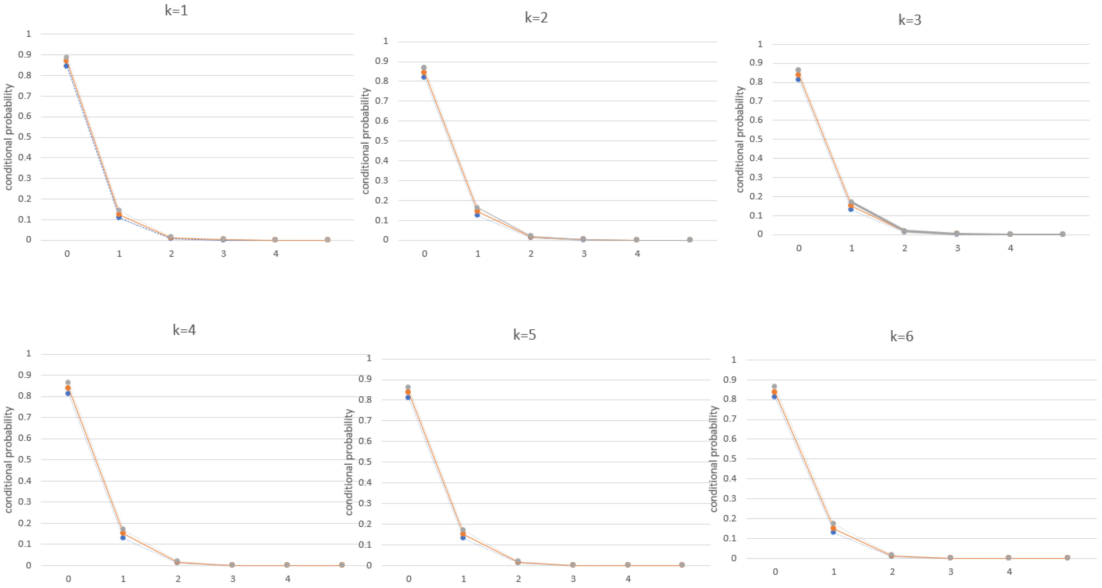
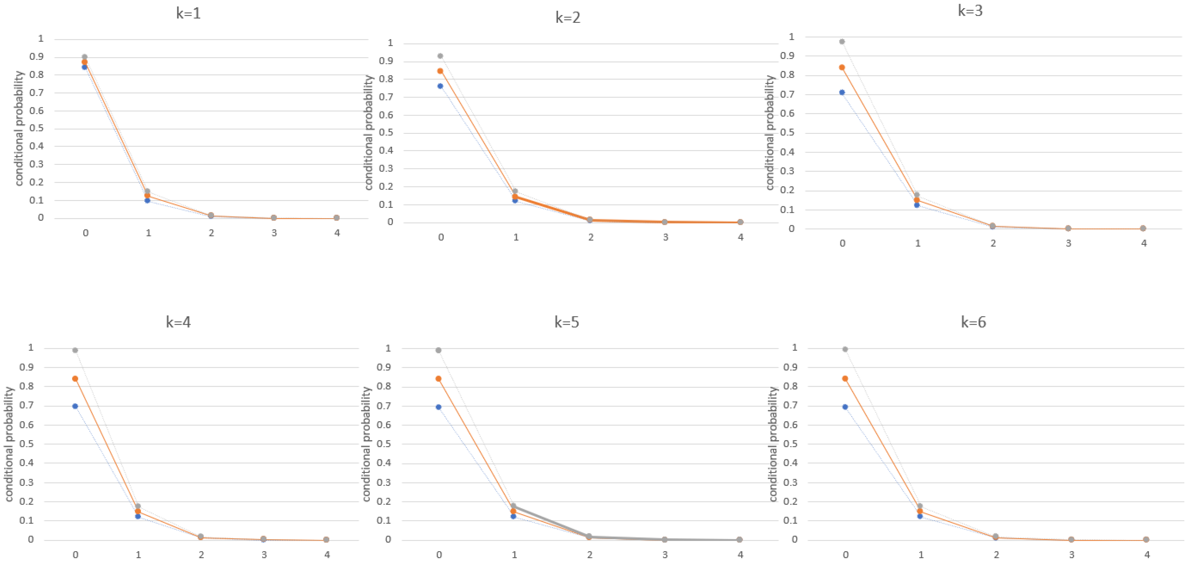
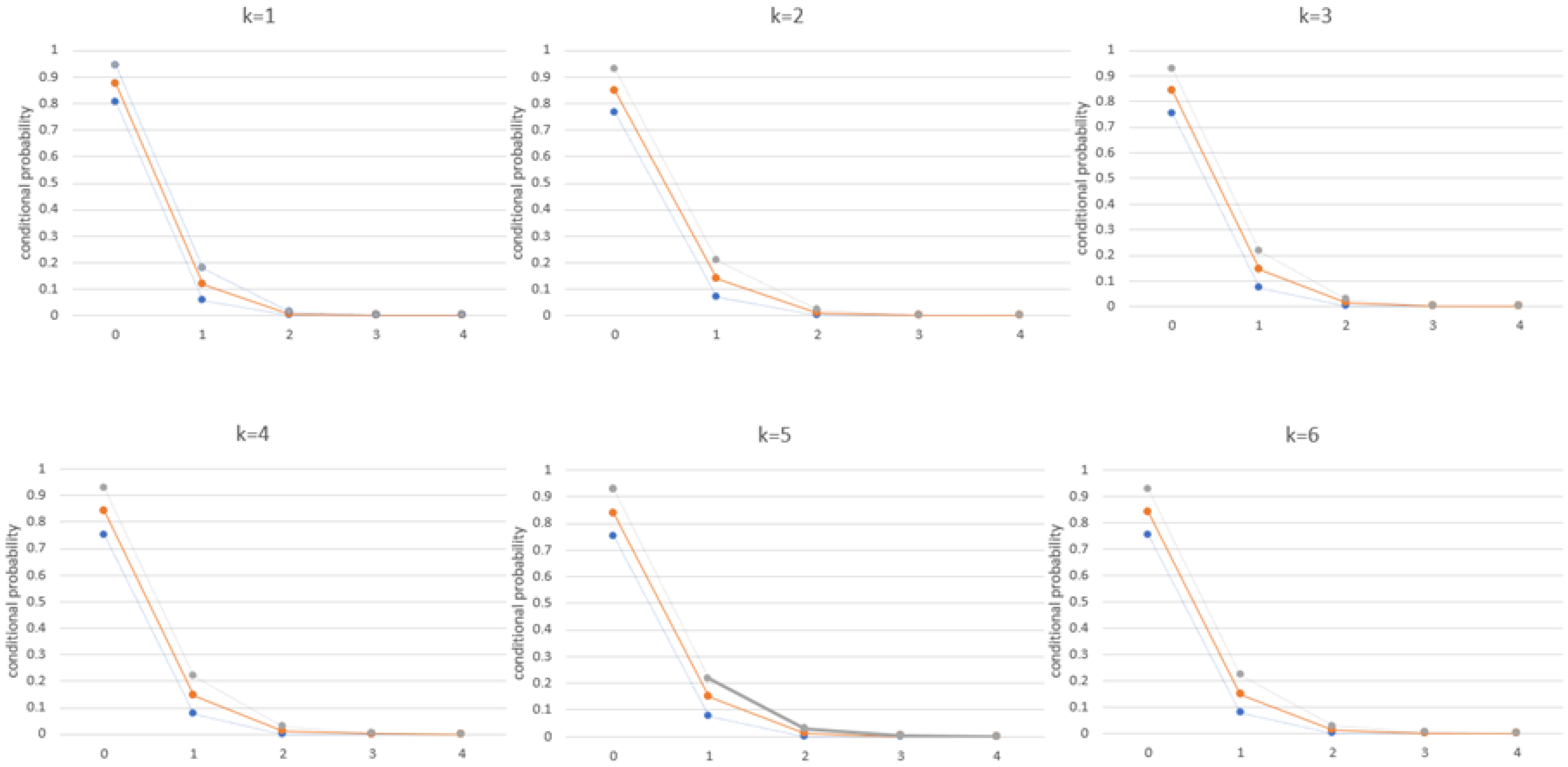
4. Coherent Forecasting

4.1. Descriptive Measures

Unlike the Box–Jenkins’ time series models which usually predict real values via conditional mean, the aim of applying coherent forecasting is to obtain an integer forecast. We applied three descriptive measures for coherent forecasting, that is, prediction root mean squared error (PRMSE), prediction mean absolute deviation (PMAD), and percentage of true prediction (PTP). Let $Y_{t+k}$ be the observation at time point $t+k$, and ${\hat{Y}}_{t+k}$ be the predicted observation, and $m$ is the number of iterations. The descriptive measures are calculated based on conditional mean and conditional median. The measures are as follows:

A.

Prediction root-mean-squared error (PRMSE):

$$\mathrm{PRMSE}=\sqrt{\frac{1}{m}{{\displaystyle \sum }}_{k=1}^m{\left(Y_{t+k}-{\hat{Y}}_{t+k}\right)}^2}$$

B.

Prediction mean absolute deviation (PMAD):

$$\mathrm{PMAD}=\frac{1}{m}{{\displaystyle \sum }}_{k=1}^m\left|Y_{t+k}-{\hat{Y}}_{t+k}\right|$$

C.

Percentage of true prediction (PTP):

$$\mathrm{PTP}=\frac{1}{m}{{\displaystyle \sum }}_{k=1}I\left(Y_{t+k}-{\hat{Y}}_{t+k}\right)\times 100\%$$

where $I(\cdot )$ is the indicator function.

4.2. Confidence Interval

We derive the 95% confidence interval for the $k$-step-ahead probability distribution function for MPT(1) model based on the asymptotic normal distribution.

Theorem 2.

Consider the k-step-ahead conditional probability$p_k(x|X_n;{\widehat{\theta }}_n)$. For a sample size$n$and fixed$x$, it has an asymptotically normal distribution with$p_k(x|X_n;{\theta }_0)$and variance

$$\begin{gathered} {\sigma }_k{}^2\left(x; {\alpha }_0, {\lambda }_0, {\varphi }_0\right)=n^{-1}[{\nu }_{\alpha }{\left({\frac{\partial p_k}{\partial \alpha }|}_{\alpha ={\alpha }_0, \lambda ={\lambda }_0,\varphi ={\varphi }_0}\right)}^2+{\nu }_{\lambda }{\left({\frac{\partial p_k}{\partial \lambda }|}_{\alpha ={\alpha }_0, \lambda ={\lambda }_0,\varphi ={\varphi }_0}\right)}^2 \\ \hspace{1em}\hspace{1em}\hspace{1em}\hspace{1em}\hspace{1em}\hspace{1em}+{\nu }_{\varphi }{\left({\frac{\partial p_k}{\partial \varphi }|}_{\alpha ={\alpha }_0, \lambda ={\lambda }_0,\varphi ={\varphi }_0}\right)}^2+2{\nu }_{\alpha \lambda }\frac{\partial p_k}{\partial \alpha }{\frac{\partial p_k}{\partial \lambda }|}_{\alpha ={\alpha }_0, \lambda ={\lambda }_0,\varphi ={\varphi }_0} \\ \hspace{1em}\hspace{1em}\hspace{1em}\hspace{1em}\hspace{1em}\hspace{1em}\hspace{1em}+2{\nu }_{\alpha \varphi }\frac{\partial p_k}{\partial \alpha }{\frac{\partial p_k}{\partial \varphi }|}_{\alpha ={\alpha }_0, \lambda ={\lambda }_0,\varphi ={\varphi }_0}+2{\nu }_{\lambda \varphi }\frac{\partial p_k}{\partial \lambda }{\frac{\partial p_k}{\partial \varphi }|}_{\alpha ={\alpha }_0, \lambda ={\lambda }_0,\varphi ={\varphi }_0}] \end{gathered}$$

where ${\nu }_{\alpha }$, ${\nu }_{\lambda }$ and ${\nu }_{\varphi }$ are the diagonal elements and ${\nu }_{\alpha \lambda }$, ${\nu }_{\alpha \varphi }$ and ${\nu }_{\lambda \varphi }$ are respectively the off-diagonal elements of $v$ in Theorem 1. The elements of the partial derivatives are

$$\begin{gathered} \frac{\partial }{\partial \alpha }{p}_k\left(x|X_n\right)=\frac{{\varphi }^{k}k{\alpha }^{k-1}{X}_n}{1-{\alpha }^k}\left(\left(\begin{array}{c}{X}_n-1\\ x-1\end{array}\right){\left({\alpha }^k\right)}^{x-1}{\left(1-{\alpha }^k\right)}^{X_n-x}-\left(\begin{array}{c}{X}_n\\ x\end{array}\right){\left({\alpha }^k\right)}^x{\left(1-{\alpha }^k\right)}^{X_n-x}\right) \\ -\lambda {\varphi }^{k}k{\alpha }^{k-1}\left(\frac{e^{-\lambda {\alpha }^k}{\left(\lambda {\alpha }^k\right)}^{x-1}}{\left(x-1\right)!}-\frac{e^{-\lambda {\alpha }^k}{\left(\lambda {\alpha }^k\right)}^x}{x!}\right)\hspace{1em}\hspace{1em} \\ \frac{\partial }{\partial \lambda }{p}_k\left(x|X_n\right)=\frac{e^{-\lambda }{\left(\lambda \right)}^{x-1}}{\left(x-1\right)!}-\frac{e^{-\lambda }{\left(\lambda \right)}^x}{\left(x\right)!}-{\left(\alpha \varphi \right)}^k\left(\frac{e^{-\lambda {\alpha }^k}{\left(\lambda {\alpha }^k\right)}^{x-1}}{\left(x-1\right)!}-\frac{e^{-\lambda {\alpha }^k}{\left(\lambda {\alpha }^k\right)}^x}{x!}\right) \\ \frac{\partial }{\partial \varphi }{p}_k\left(x|X_n\right)=k{\varphi }^{k-1}\left[\left(\begin{array}{c}{X}_n\\ x\end{array}\right){\left({\alpha }^k\right)}^x{\left(1-{\alpha }^k\right)}^{X_n-x}-\frac{e^{-\lambda {\alpha }^k}{\left(\lambda {\alpha }^k\right)}^x}{x!}\right] \end{gathered}$$

Thus, a 95% confidence interval for $p_k(x|X_n; {\alpha }_0, {\lambda }_0, {\varphi }_0)$, based on its asymptotic distribution, is given by

$$p_k\left(x|X_n; {\hat{\alpha }}_n, {\hat{\lambda }}_n, {\hat{\varphi }}_n\right)\pm 1.96{\sigma }_k\left(x; {\alpha }_0, {\lambda }_0, {\varphi }_0\right)$$

5. Simulation Study

A simulation study was conducted to compare the coherent forecasting performance for all models presented in Section 2, that is, MPT(1), INAR(1) and Pegram’s AR(1) with Poisson marginal. The data for this simulation study were generated from Pegram’s AR(1) process with geometric marginal with parameters $\left(0.5,0.4\right)$ to represent low count series, and $\left(0.3,0.8\right)$ to represent high count series. A sample size of 1000 for 10,000 Monte Carlo samples was considered for the three models with Poisson marginal, that is, INAR(1), Pegram’s AR(1) and MPT(1).

Given a $\left(n+m\right)$ size of observed data $\left\{x_1,x_2,\dots ,x_n,x_{n+1},\dots x_{n+m}\right\}$, the data were partitioned into the training set $\left\{x_1,x_2,\dots ,x_n\right\}$ and test set $\left\{x_{n+1},\dots x_{n+m}\right\}$. The training set was used to estimate the parameters whilst the test set was used to measure the forecasting performance. We divided the simulated data into 70% for the training set and 30% for the test set. The simulation results with 10,000 Monte Carlo samples are reported in

Table 1. Estimated PRMSE, PMAD and PTP for Pegram’s AR(1), INAR(1) and MPT(1), with Poisson process.

Model	Parameters	PRMSE	PMAD	PTP (%)
Pegram’s AR(1)	(0.5,0.4)	0.0867	1.6135	22.3474
	(0.3,0.8)	0.0335	0.4000	66.7706
INAR(1)	(0.5,0.4)	0.9952	2.0921	14.8930
	(0.3,0.8)	0.0341	0.3997	65.0158
MPT(1)	(0.5,0.4)	0.1482	1.4890	23.6388
	(0.3,0.8)	0.02446	0.4528	59.4330

. In the simulation study, the models were misspecified because data were generated from Pegram’s AR(1) process with geometric marginal. It is known that multi-step ahead forecasting is robust to model misspecification [23]. To check for robustness, the error measures were computed for 50, 100 and 300 steps ahead of forecasting. It was seen that there was little difference in the errors.

First, we compared the forecasting accuracy of the model for different parameters. Table 1 exhibits the simulation results of a 10,000 sample size for estimated PRMSE, PMAD and PTP for the MPT(1) model. It was seen that the percentage of true prediction (PTP) for high count series is much higher than low count series. The PMAD was recorded as 0.45 for high count series, which is much lower than 1.49 for low count series. Similarly, for PRMSE, the error is 2% for high count series compared to a 14% error for low count series.

Next, we compared the forecasting accuracy across the time series models. For high count series, it was highlighted that the PTP of MPT(1) outperformed the other two models, and for low count series, MPT(1) model obtained about 24% of correct predictions which was slightly better than Pegram’s AR(1) model, and performing much better than INAR(1) model. A summary that can be drawn from the simulation study is that the MPT(1) model is better equipped to handle low count series, whilst remaining competent for high count series. We show some potential applications in the next section.

6. Real Applications

In this section, real data application is considered to illustrate the feasibility of the model. Two real data sets are used in the analysis. Both data sets are equi-dispersed. This section aims to study the forecasting performance of the MPT(1), INAR(1) and Pegram’s AR(1) models for both sets of data. For all three models, we consider Poisson marginal distribution.

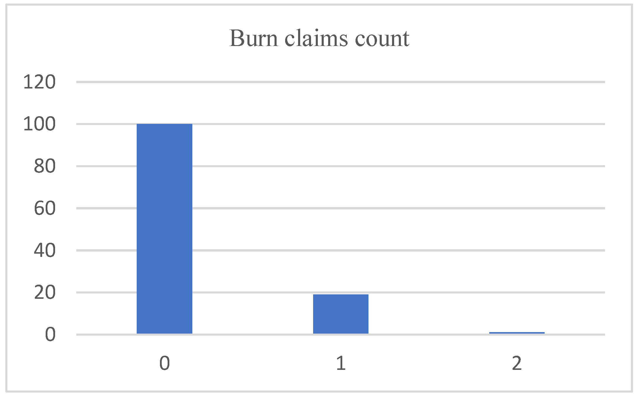
6.1. Burn Claims Data

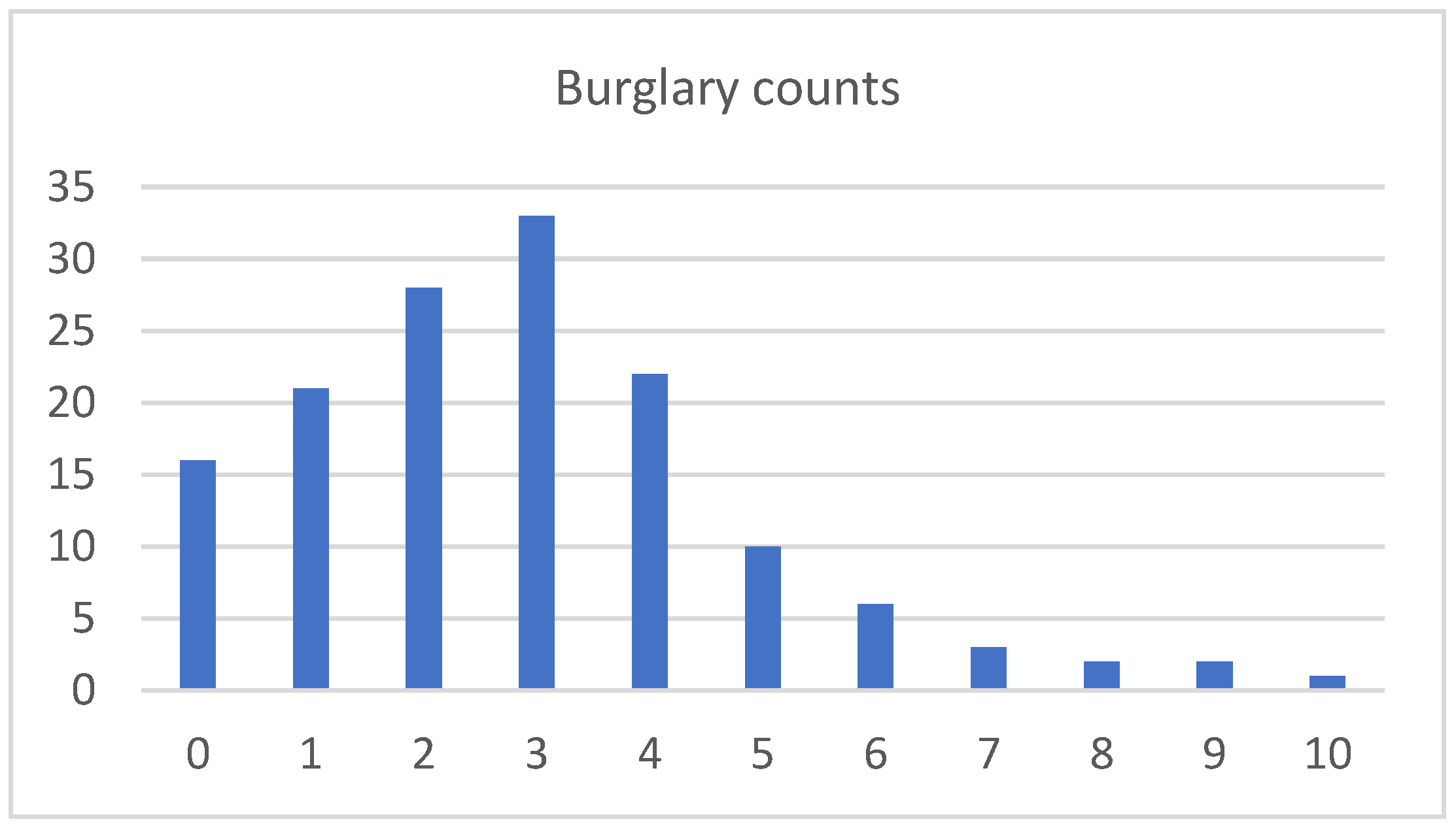
This data set was taken from the Workers Compensation Board (WCB) of British Columbia in Canada. The data considered only the male workers, aged between 35 to 54, in a logging company. The sample size was 120, and data were collected monthly from January 1984 to December 1994. The frequency of the data is provided in Figure 1. The data set contained high counts of zero, with 100 zeros out of 120 observations, and the maximum is 2, which has only two counts. The mean of 0.34 is virtually equal to the variance of 0.33, suggesting that fitting with Poisson marginal is feasible. The model comparison was carried out among MPT, Pegram’s AR(1) and INAR(1). In the comparison, the focus was on forecasting accuracy.

For the data consisting of 120 observations, 110 observations were allocated to the training set and the remaining 10 observations were used for the testing set. We estimated the parameters from the training data set, and the forecasting accuracy was computed based on the testing set. All the models provided similar results. It was reported that no observations in the testing set were predicted correctly. The computation for PRMSE and PMAD was 1.3784 and 1.3, respectively.

We performed a study to compare the forecasting performance with conditional mean and conditional median. The results are tabulated in

Table 2. Comparison of forecasting performance with conditional mean and conditional median.

Model		Conditional Mean	Conditional Median
MPT(1)	PRMSE	0.5492	1.3784
	PMAD	0.3152	1.3
	PTP (%)	50	0
Pegram’s AR(1)	PRMSE	1.0585	1.3784
	PMAD	0.9511	1.3
	PTP (%)	0	0
INAR(1)	PRMSE	0.9037	1.3784
	PMAD	0.7359	1.3
	PTP (%)	0	0

. It was reported that the conditional mean (rounded up to the nearest integer) for MPT(1) model, outperformed the other models, with lower PRMSE and PMAD. In addition, the PTP had a 50% of true prediction. It is recommended that for MPT(1) model, the conditional mean can be a viable tool for forecasting, with simpler expression and better accuracy compared to the conditional median.

Next, we were provided with some extra information on the asymptotic forecasting distribution for all models. The parameter estimation of the Poisson MPT(1) process was conducted with the EM algorithm for the computation of 95% confidence intervals. The parameters and the standard errors (in brackets) for burn claims were estimated to be $\hat{\alpha }=0.9979\left(0.0245\right)$, $\hat{\varphi }=0.1789\left(0.0001\right)$ and $\hat{\lambda }=0.1792\left(0.0052\right)$. For coherent forecasting, we applied k-step-ahead distributions of MPT(1) for the burn claims data, and the 95% confidence intervals were computed. Figure 2, Figure 3 and Figure 4 show the conditional probability for the first six months.

All the models performed well for low count data in coherent forecasting. Then, 10-step-ahead forecasting was run to observe the overall performance of the models. It was noticed that the conditional distribution converged to the marginal distribution after six steps. It was reported that the probability of zero claims in the first month was about 87%. The computation also generated an average of 84% of no claims in the first five months. Comparatively, it was highlighted that the standard error of the conditional probability estimates by the MPT(1) process was 3.9% lower than Pegram’s AR(1), and was 2.5% lower than INAR(1) models.

6.2. Burglary Data

In this data set, the highest frequency of count is 3 and involved only one large observation of 10. The burglary data were taken from the unique ID of the Beat 11 of Pittsburgh city. The duration of the data was from the year 1990–2001. The mean of the data was 2.8819 and the variance was 2.9652, which had an index of dispersion of 1.0289. The sample PACF showed that lag 1 was possible, suggesting the fitting with Poisson MPT(1) model. Figure 5 shows the frequency distribution of the data.

The data were split into 132 counts for training purposes, and the remaining 12 counts were kept for testing. For the Poisson MPT(1) model, it was observed that PRMSE was 1.6073, PMAD was 1.25 and PTP was 25%. Similar results were obtained for Pegram’s AR(1) and INAR(1) with Poisson marginals.

7. Final Remarks

This paper examined coherent forecasting of Poisson MPT(1), a mixture model proposed by [1]. The k-step-ahead conditional probability function and the relevant properties were considered. Specifically, likelihood-based asymptotic distribution was developed for the Poisson MPT(1) process. Three descriptive measures in forecasting based on the conditional mean and conditional median were considered to measure the performance of forecasting, that is, PRMSE, PMAD and PTP.

A simulation study was conducted to evaluate the forecasting performance for MPT(1), Pegram’s AR(1) and INAR(1) models with Poisson marginal. From the simulation study, MPT(1) exhibited good forecasting performance. To exemplify the application, two real data sets were used. For low count series, the conditional mean of the MPT(1) process provided a more desirable forecast compared to the conditional median. An added computational advantage was the simpler expression for the conditional mean.

The results highlighted that the k-step-ahead conditional probability function and k-step-ahead conditional mean quickly converge to the probability function and the mean after 4-step-ahead, respectively. The simulation study demonstrated that the multi-step forecasting approach is robust to model misspecification. To conclude, Poisson MPT(1) process is a flexible and viable integer-valued time series model with good coherent forecasting performance.

References

1. Khoo, W.C.; Ong, S.H.; Biswas, A. Modeling time series of counts with a new class of INAR(1) model. Stat. Pap. 2017, 58, 393–416. [Google Scholar] [CrossRef]
2. Shirozhan, M.; Mohammadpour, M. An INAR(1) model based on the Pegram and thinning operators with serially dependent innovation. Commun. Stat. Simul. Comput. 2020, 49, 2617–2638. [Google Scholar] [CrossRef]
3. Kang, Y.; Wang, D.; Yang, K. A new INAR(1) process with bounded support for counts showing equidispersion, underdispersion and overdispersion. Stat. Pap. 2021, 62, 745–767. [Google Scholar] [CrossRef]
4. Yan, H.; Wang, D.H.; Li, C. A study for the NMBAR(1) processes. Commun. Stat. Simul. Comput. 2022, 1–22. [Google Scholar] [CrossRef]
5. McKenzie, E. Some simple models for discrete variate time series. Water Resour. Bull. 1985, 21, 645–650. [Google Scholar] [CrossRef]
6. Freeland, R.K. Statistical Analysis of Discrete Time Series with Application to the Analysis of Workers’ Compensation Claims Data. Ph.D. Thesis, The University of British Columbia, Vancouver, BC, Canada, 1998. [Google Scholar]
7. Freeland, R.K.; McCabe, B.P.M. Forecasting discrete valued low count time series. Int. J. Forecast. 2004, 20, 427–434. [Google Scholar] [CrossRef]
8. Bu, R.B.; McCabe, B.; Hadri, K. Maximum likelihood estimation of higher-order integer-valued autoregressive process. J. Time Ser. Anal. 2009, 29, 973–994. [Google Scholar] [CrossRef]
9. McCabe, B.P.M.; Martin, G.M. Bayesian predictions of low count time series. Int. J. Forecast. 2005, 21, 315–330. [Google Scholar] [CrossRef]
10. Jung, R.C.; Tremayne, A.R. Coherent forecasting in integer time series models. Int. J. Forecast. 2006, 22, 223–238. [Google Scholar] [CrossRef]
11. Kim, H.Y.; Park, Y. Markov chain approach to forecast in the binomial autoregressive models. Commun. Korean Stat. Soc. 2010, 17, 441–450. [Google Scholar] [CrossRef]
12. Maiti, R.; Biswas, A.; Das, S. Coherent forecasting for count time series using Box-Jenkins’s AR(p) model. Stat. Neerl. 2016, 70, 123–145. [Google Scholar] [CrossRef]
13. Maiti, R.; Biswas, A.; Das, S. Time series of zero-inflated counts and their coherent forecasting. J. Forecast. 2015, 34, 694–707. [Google Scholar] [CrossRef]
14. Awale, M.; Ramanathan, T.V.; Kale, M. Coherent forecasting in integer-valued AR(1) models with geometric marginals. J. Data Sci. 2017, 15, 95–114. [Google Scholar] [CrossRef]
15. Nik, S.; Weiss, C. CLAR(1) point forecasting under estimation uncertainty. Stat. Neerl. 2020, 74, 489–526. [Google Scholar] [CrossRef]
16. Weiss, C. Thinning operations for modelling time series of counts—A survey. AStA Adv. Stat. Anal. 2008, 92, 319. [Google Scholar] [CrossRef]
17. Pegram, G.G.S. An autoregressive model for multilag Markov chain. J. Appl. Probab. 1980, 17, 350–362. [Google Scholar] [CrossRef]
18. Biswas, A.; Song, X.-K. Peter. Discrete-valued ARMA processes. Stat. Probab. Lett. 2009, 79, 1884–1889. [Google Scholar] [CrossRef]
19. Jacobs, P.A.; Lewis, A.W. Discrete Time Series Generated by Mixtures III: Autoregressive Processes (DAR(p)); Naval Postgraduate School: Monterey, CA, USA, 1978. [Google Scholar]
20. Grunwald, G.K.; Hyndman, R.J.; Tedesco, L.; Tweedie, R.L. Non-Gaussian conditional linear AR(1) models. Aust. N. Z. J. Stat. 2000, 42, 479–495. [Google Scholar] [CrossRef]
21. Dempster, A.; Laird, N.; Rubin, D. Maximum Likelihood from Incomplete Data via the EM Algorithm. J. R. Stat. Soc. B 1977, 39, 1–38. [Google Scholar]
22. Karlis, D.; Xekalaki, E. Improving the EM algorithm for mixtures. Stat. Comput. 1999, 9, 303–307. [Google Scholar] [CrossRef]
23. Marcellino, M.; Stock, J.H.; Watson, M.W. A comparison of direct and iterated multistep AR methods for forecasting macroeconomic time series. J. Econ. 2006, 135, 499–526. [Google Scholar] [CrossRef]
Figure 1. The histogram of the burn claims data.
Mathematics 10 02961 g001
Figure 2. Forecasted conditional probability with 95% confidence interval by MPT(1).
Mathematics 10 02961 g002
Figure 3. Forecasted conditional probability with 95% confidence interval by Pegram AR(1).
Mathematics 10 02961 g003
Figure 4. Forecasted conditional probability with 95% confidence interval by INAR(1).
Mathematics 10 02961 g004
Figure 5. Frequency distribution plot of burglary counts.
Mathematics 10 02961 g005