Event-Triggered Non-PDC Filter Design of Fuzzy Markovian Jump Systems under Mismatch Phenomena

Abstract

This paper focuses on dealing with the problem of co-designing a fuzzy-basis-dependent event generator and an asynchronous filter of fuzzy Markovian jump systems via event-triggered non-parallel distribution compensation (non-PDC) scheme. The introduction of the event-triggered non-PDC scheme can reduce the number of real-time filter gain design operations with a large computational load. Furthermore, to perform an effective relaxation process, several kinds of time-varying parameters in filter design conditions are simultaneously relaxed by utilizing two zero equalities of transition probabilities and mismatch errors. In addition, to improve the considered performance, the event generation function is established based on fuzzy-basis-dependent event weighting matrices.

1. Introduction

As is well known, the Markovian jump system model has the advantage that it is very suitable for characterizing dynamic hybrid systems with abrupt parameters or structural changes (see [1,2,3,4]). Furthermore, it has also been recognized that the T-S fuzzy system model has an excellent ability to represent nonlinear systems by blending local linear systems (refer to [5,6,7,8,9,10,11]). In this context, fuzzy Markovian jump systems (FMJSs) have become quite popular because these systems can systematically fuse the unique features of the above two system models. Accordingly, the FMJSs have been actively utilized in various application systems where nonlinearity and system mode change must be considered, for example in fields such as robotic, communication, network control, economic system, and power system [12,13,14,15,16,17,18]. In particular, as reported in [19,20,21], the introduction of the non-PDC scheme offers the advantage of decreasing the conservatism of the controller or filter design conditions. Thus, in light of the non-PDC scheme, Ref. [22] developed the robust mode-independent state-feedback controller for homogeneous FMJSs, and Ref. [23] designed the super-twisting controller for descriptor homogeneous FMJSs via integral sliding modes. In addition, Ref. [24] addressed the problem of synchronous mode-dependent observer-based control for fractional-order fuzzy systems with homogeneous Markov process via the non-PDC scheme. Most recently, using the non-PDC scheme, Ref. [25] addressed the problem of dissipative controller design for nonhomogeneous FMJSs with dual modes.

However, one noteworthy point is that further investigation is still needed to consider the asynchronism and nonhomogeneity when designing filters of FMJSs according to the non-PDC scheme.

Moreover, an event-triggered mechanism has received considerable attention in recent years due to its advantages of reducing the transmitted data throughput and/or computation times. In fact, since the non-PDC scheme requires more computational load compared to the PDC scheme due to inverse matrix operations, performing such operations every time acts as a factor that reduces the efficiency of hardware resources. For this reason, the number of times to update the fuzzy filter gains also needs to be reduced by automatically activating the non-PDC and fuzzy basis function (FBF) modules according to an event-triggered mechanism. To realize this, two additional design requirements must be considered along with the filter design problem: (i) one is that the current system operation mode cannot be precisely used for filter operation, and (ii) the other is that the current premise variables of FBF cannot be accurately obtained real-time. In [26], a study of event-triggered and reduced-order filtering for homogeneous FMJSs was performed with consideration of asynchronous filter modes. In addition, Ref. [27] addressed the adaptive event-triggered finite-time filtering problem for interval type-2 homogeneous FMJSs with asynchronous modes, and Ref. [28] investigated the event-triggered asynchronous filtering problem of semi-FMJSs subject to deception attacks. Besides, under imperfect premise matching, Ref. [29] addressed the networked ${\mathcal{H}}_{\infty }$ fuzzy filtering problem of homogeneous FMJSs. Indeed, all of the above studies provide successful results in designing event-triggered and networked filters under practical constraints. However, it is also true that more attention needs to be paid to simultaneously meet the above requirements in the non-PDC filtering problem of nonhomogeneous FMJSs.

To compensate for the shortcomings of the previous studies, this paper aims to co-design a fuzzy-basis-dependent event generator and an asynchronous filter of nonhomogeneous FMJSs via an event-triggered non-PDC scheme. To this end, this paper provides a method to transform the nonconvex form of filter design conditions into the parameterized linear matrix inequality (PLMI)-based form by utilizing the congruence transformation and the matrix inequality-based decoupling method. After that, based on the proposed relaxation process, the PLMI-based conditions are transformed into the LMI-based conditions in a less conservative manner. The detailed contributions of this paper can be summarized as follows.

• In contrast to other studies based on the PDC scheme, to enhance the performance improvement, this paper uses a non-PDC scheme when designing asynchronous mode-dependent fuzzy filter gains. In addition, the mode- and fuzzy-basis-dependent event weighting matrices are employed to construct the event generation function.
• By taking the design requirements (i) and (ii) into account, this paper proposes a method such that at the moment when the event generation condition is satisfied, the system mode can be transmitted to the filter side, and the non-PDC and FBF modules can be activated. In particular, the problem of mismatched fuzzy basis functions, caused by using the event-triggered outputs as the source of premise variables on the filter side, is effectively addressed by considering their errors from the original.
• The relaxation of the PLMI-based conditions is effectively performed (i) by simultaneously addressing three types of time-varying parameters, i.e., transition probabilities, fuzzy basis functions, and mismatched fuzzy basis functions, and (ii) by reflecting two zero equalities of transition probabilities and mismatch errors in the relaxation process so that less conservative LMIs can be derived from PLMIs.

Notations: ${\mathbb{N}}_n$ denotes the set $\{1,2,\cdots ,n\}$. $P\ge 0$ ($P>0$) means that P is real symmetric and positive semidefinite (definite). In symmetric block matrices, the asterisk $(\ast )$ is used as an ellipsis for terms induced by symmetry. $\mathbf{E}\{·\}$ denotes the mathematical expectation; $\mathbf{diag}(·)$ stands for a block-diagonal matrix; $\mathbf{col}(v_1,v_2,\dots ,v_n)={[v_1^T{v}_2^T\cdots v_n^T]}^T$; $\mathbf{He}\left\{X\right\}=X+X^T$; and $I_n$ is the $n\times n$-dimensional identity matrix. ${\Lambda }_n=\left\{\mathbf{col}({\lambda }_1,\cdots ,{\lambda }_n)\in {\mathbb{R}}^n|{\lambda }_1+\cdots +{\lambda }_n=1,{\lambda }_i\ge 0,i\in {\mathbb{N}}_n\right\}$ denotes the $n-1$ dimensional standard simplex. For $\mathbb{S}=\{s_1,s_2,\cdots ,s_n\}$, the following notations are used:

$$\begin{array}{c}\hfill {\left[{\mathcal{Q}}_i\right]}_{i\in \mathbb{S}}^T=\left[\begin{array}{ccc}{\mathcal{Q}}_{s_1}^T& \cdots & {\mathcal{Q}}_{s_n}^T\end{array}\right],{\left[{\mathcal{Q}}_i\right]}_{i\in \mathbb{S}}^{\mathbf{d}}=\mathbf{diag}\left({\mathcal{Q}}_{s_1},\cdots ,{\mathcal{Q}}_{s_n}\right),\end{array}$$

where ${\mathcal{Q}}_{(·)}$ denotes a real submatrix or a scalar value.

2. System Description and Preliminaries

For a given probability space $(\Omega ,\mathcal{F},\mathbf{Pr})$, let us consider the following FMJS with the system mode $\varphi \left(k\right)\in {\mathbb{N}}_{\alpha }=\{1,2,\cdots ,\alpha \}$:

$$\begin{array}{c}\hfill \left\{\begin{array}{c}x(k+1)=A\left(\theta \right(k),\varphi (k\left)\right)x\left(k\right)+B\left(\theta \right(k),\varphi (k\left)\right)w\left(k\right),\hfill \\ y\left(k\right)=C\left(\theta \right(k),\varphi (k\left)\right)x\left(k\right)+D\left(\theta \right(k),\varphi (k\left)\right)w\left(k\right),\hfill \\ z\left(k\right)=E\left(\theta \right(k),\varphi (k\left)\right)x\left(k\right),\hfill \end{array}\right.\end{array}$$

(1)

where $x\left(k\right)\in {\mathbb{R}}^{n_x}$, $w\left(k\right)\in {\mathbb{R}}^{n_w}$, $y\left(k\right)\in {\mathbb{R}}^m$, and $z\left(k\right)\in {\mathbb{R}}^{n_z}$ denote the state, the disturbance input that belongs to ${\mathfrak{L}}_2[0,\infty )$, the measurement output, and the performance output; $\varphi \left(k\right)$ is characterized by a discrete-time Markov chain operating according to ${\pi }_{gh}\left(k\right)=\mathbf{Pr}({\varphi }_{k+1}=h|{\varphi }_k=g)$; and for $\varphi \left(k\right)=g$,

$$\begin{array}{cc}\hfill & A(\theta \left(k\right),\varphi \left(k\right))=\sum _{i=1}^r{\theta }_i\left(\eta \left(k\right)\right)A_{gi},B(\theta \left(k\right),\varphi \left(k\right))=\sum _{i=1}^r{\theta }_i\left(\eta \left(k\right)\right)B_{gi},\hfill \\ \hfill & C(\theta \left(k\right),\varphi \left(k\right))=\sum _{i=1}^r{\theta }_i\left(\eta \left(k\right)\right)C_{gi},D(\theta \left(k\right),\varphi \left(k\right))=\sum _{i=1}^r{\theta }_i\left(\eta \left(k\right)\right)D_{gi},\hfill \\ \hfill & E(\theta \left(k\right),\varphi \left(k\right))=\sum _{i=1}^r{\theta }_i\left(\eta \left(k\right)\right)E_{gi},\hfill \end{array}$$

in which $\theta \left(k\right)=\mathbf{col}({\theta }_1\left(\eta \left(k\right)\right),{\theta }_2\left(\eta \left(k\right)\right),\cdots ,{\theta }_r\left(\eta \left(k\right)\right))$ denotes the normalized fuzzy basis (or called fuzzy weighting) function vector goverend by the premise variable $\eta \left(k\right)$; and r denotes the number of IF-THEN fuzzy rules. Specifically, in (1), $\theta \left(k\right)$ and ${\pi }_g\left(k\right)=\mathbf{col}({\pi }_{g1}\left(k\right),{\pi }_{g2}\left(k\right),\cdots ,{\pi }_{g\alpha }\left(k\right))$ satisfy $\theta \left(k\right)\in {\Lambda }_r$ and ${\pi }_g\left(k\right)\in {\Lambda }_{\alpha }$. Furthermore, to consider realistic situations, the mode set of $h\in {\mathbb{N}}_{\alpha }$ is classified into two subsets such that ${\mathbb{N}}_{\alpha }={\mathbb{H}}_g\bigcup {\tilde{\mathbb{H}}}_g$:

$$\begin{array}{cc}\hfill {\mathbb{H}}_g& =\left\{h\in {\mathbb{N}}_{\alpha }|{\pi }_{gh}\left(k\right) \mathrm{is} \mathrm{time}-\mathrm{invariant} \mathrm{as} {\pi }_{gh} \mathrm{and} \mathrm{completely} \mathrm{known}\right\},\hfill \\ \hfill {\tilde{\mathbb{H}}}_g& =\left\{h\in {\mathbb{N}}_{\alpha }|{\pi }_{gh}\left(k\right) \mathrm{is} \mathrm{bounded} \mathrm{as} \in [{\underline{\pi }}_{gh},{\overline{\pi }}_{gh}]\right\},\hfill \end{array}$$

(2)

where ${\tilde{\mathbb{H}}}_g$ contains the set $\{h\in {\mathbb{N}}_{\alpha }|{\pi }_{gh}\left(k\right) \mathrm{is} \mathrm{completely} \mathrm{unknown}\}$ because the transition probability essentially satisfies ${\pi }_{gh}\left(k\right)\in [0,1]$.

Next, let us consider the following output error between the current and transmitted outputs, caused by the event-triggered mechanism:

$$\begin{array}{c}\hfill \overline{y}\left(k\right)=y\left(k\right)-y\left(s_p\right),\end{array}$$

(3)

where $s_p$ indicates the last transfer time instance and $p\in \{0,1,2,\cdots \}$ represents the corresponding index number. Based on the output error, the event-triggered mechanism operates according to the following fuzzy-basis-dependent event generation function:

$$\begin{array}{c}\hfill f(y\left(k\right),y\left(s_p\right))={\overline{y}}^T\left(k\right)S_g\left(\theta \left(k\right)\right)\overline{y}\left(k\right)-y^T\left(k\right)\left({\Gamma }_g{S}_g\left(\theta \left(k\right)\right)\right)y\left(k\right),\end{array}$$

(4)

where $S_g\left(\theta \left(k\right)\right)>0$ denotes the fuzzy-basis-dependent event weighting matrix to be determined later, and ${\Gamma }_g=\mathbf{diag}({\gamma }_{g1},{\gamma }_{g2},\cdots ,{\gamma }_{gm})$ denotes the given event threshold matrix with ${\gamma }_{gi}\in [0,1]$ for all $i\in {\mathbb{N}}_m$. In other words, the transmission of both output and system mode is triggered at the following time instance:

$$\begin{array}{c}\hfill s_{p+1}=\underset{k}{inf}\left\{k>s_p|f(y\left(k\right),y\left(s_p\right))>0\right\}.\end{array}$$

(5)

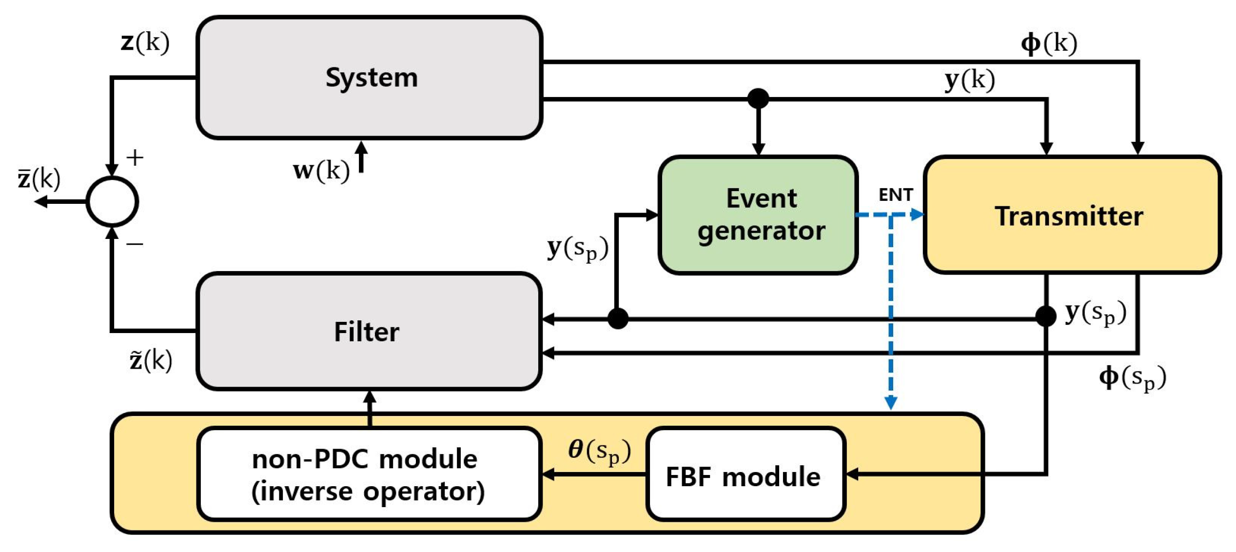
As shown in Figure 1, this paper aims to design a filter that estimates the performance output $z\left(k\right)$ using the measured output $y\left(k\right)$ under an event-triggered mechanism. The event-triggered mechanism is operated through the event generator and the transmitter, where the event generator outputs an ENT signal to the transmitter at the moment (5) holds (i.e., at $k=s_p$), and the transmitter is activated by the ENT signal and sends the measured output signal $y\left(s_p\right)$ and system mode $\varphi \left(s_p\right)$ to the next modules. In particular, the FBF module is used to construct the event-triggered fuzzy basis function $\theta \left(s_p\right)=\mathbf{col}({\theta }_1\left(s_p\right),{\theta }_2\left(s_p\right),\cdots ,{\theta }_r\left(s_p\right))$ from the transmitted output $y\left(s_p\right)$, and the non-PDC module calculates the $\tilde{\theta }$-dependent filter gains using the inverse operation.

Remark 1.

The event generator performs calculations (3) and (4), and then generates an ENT signal at the moment (5) holds. With a cascade connection, the transmitter is activated by the ENT signal and sends the measured output $y\left(s_p\right)$ and system mode $\varphi \left(s_p\right)$ to the filter and the FBF module.

Remark 2.

As can be seen from Figure 1, the role of the ENT signal can be specifically divided into two categories. The first is to determine the timing at which the transmitter is activated. When the transmitter is activated, the triggered output signal $y\left(s_p\right)$ and $\varphi \left(s_p\right)$ can be sent to the next modules. The second is to activate the filter gain update process consisting of the FBF module and the non-PDC module. Ultimately, the ENT-based update process can reduce the number of inverse operations to be driven in the non-PDC module.

Constraint 1.

To reduce data throughput, this paper proposes a protocol that allows the system mode $\varphi \left(k\right)$ to be transmitted to the filter side at time instance $k=s_p$. Thereupon, the filter mode is maintained at $\varphi \left(s_p\right)$ for $k\in [s_p,s_{p+1})$, which becomes asynchronous with the system mode $\varphi \left(k\right)$ for that time interval. In this regard, as a form of representing the asynchronism between $\varphi \left(k\right)$ and $\varphi \left(s_p\right)$, this paper employs the following conditional probability:

$$\begin{array}{c}\hfill \mathbf{Pr}\left(\varphi \left(s_p\right)=\ell |\varphi \left(k\right)=g\right)={\varpi }_{g\ell },\forall g,\ell \in {\mathbb{N}}_{\alpha },\end{array}$$

(6)

which satisfies ${\varpi }_g=\mathbf{col}({\varpi }_{g1},{\varpi }_{g2},\cdots ,{\varpi }_{g\alpha })\in {\Lambda }_{\alpha }$. In practice, one can utilize the relative frequency distribution method [30] to construct ${\varpi }_{g\ell }$ from data for $(\varphi \left(k\right),\varphi \left(s_p\right))$ pairs.

Constraint 2.

In the considered protocol, since the output signal is transmitted to the filter side only at $k=s_p$, the fuzzy basis function must be constructed using the transmitted output $y\left(s_p\right)$ via the FBF module in Figure 1, and the fuzzy-basis-dependent filter has no choice but to be designed on the basis of $\theta \left(s_p\right)=\mathbf{col}({\theta }_1(\eta \left(s_p\right),\cdots ,{\theta }_r\left(\eta \left(s_p\right)\right))\in {\Lambda }_r$ via the non-PDC module in Figure 1. Meanwhile, since the mismatched fuzzy basis function $\theta \left(s_p\right)$ is given from $\theta \left(k\right)$, the following properties still hold: ${\sum }_{i=1}^r{\theta }_i\left(s_p\right)=1$ and $0\le {\theta }_i\left(s_p\right)\le 1$, for all $i\in {\mathbb{N}}_r$. Thus, the mismatch error ${\delta }_i\left(k\right)={\theta }_i\left(k\right)-{\theta }_i\left(s_p\right)$ satisfies

$$\begin{array}{cc}\hfill & \sum _{i=1}^r{\delta }_i\left(k\right)=0,|{\delta }_i\left(k\right)|\le {\overline{\delta }}_i\le 1,\forall i\in {\mathbb{N}}_r.\hfill \end{array}$$

(7)

where ${\overline{\delta }}_i$ is introduced as a tunable upper bound to improve filtering performance. In practice, the setting of ${\overline{\delta }}_i$ will be verified via the transient responses of ${\theta }_i\left(k\right)$ and ${\theta }_i\left(s_p\right)$.

Remark 3.

Since the fuzzy basis function of filter, i.e., $\theta \left(s_p\right)$, corresponds to an instantaneous value of $\theta \left(k\right)$ at $k=s_p$, it still follows the fundamental properties of $\theta \left(k\right)$, that is, ${\sum }_{i=1}^r{\theta }_i\left(s_p\right)=1$ and $0\le {\theta }_i\left(s_p\right)\le 1$, for all $i\in {\mathbb{N}}_r$.

By considering (2)–(7), subject to Constraints 1 and 2:

$$\begin{array}{c}\hfill \left\{\begin{array}{cc}\tilde{x}(k+1)\hfill & =F(\theta \left(s_p\right),\varphi \left(s_p\right))\tilde{x}\left(k\right)+G(\theta \left(s_p\right),\varphi \left(s_p\right))y\left(s_p\right),\hfill \\ \tilde{z}\left(k\right)\hfill & =H(\theta \left(s_p\right),\varphi \left(s_p\right))\tilde{x}\left(k\right),\hfill \end{array}\right.\end{array}$$

(8)

where $\tilde{x}\left(k\right)\in {\mathbb{R}}^{n_{\tilde{x}}}$ and $\tilde{z}\left(k\right)\in {\mathbb{R}}^{n_z}$ denote the filter state and the estimated performance output, respectively; $\varphi \left(s_p\right)$ stands for the asynchronous filter mode; and the filter gains $F(\theta \left(s_p\right),\varphi \left(s_p\right))$, $G(\theta \left(s_p\right),\varphi \left(s_p\right))$, and $H(\theta \left(s_p\right),\varphi \left(s_p\right))$ are obtained later according to the non-PDC scheme [20].

Remark 4.

In comparison to PDC, the non-PDC scheme demands more computational burden to calculate the fuzzy filter gains. Thus, based on (8), this paper proposes a method such that $\tilde{z}\left(k\right)$ follows $z\left(k\right)$ even if the filter gains are updated only when the output is transmitted (i.e., at time instance $k=s_p$.

Before going ahead, for the sake of simplicity, we use the following notations hereafter: $\theta =\theta \left(k\right)$, ${\theta }_i={\theta }_i\left(\eta \left(k\right)\right)$, ${\theta }^{+}=\theta (k+1)$, ${\theta }_i^{+}={\theta }_i(k+1)$, $\tilde{\theta }=\theta \left(s_p\right)$, ${\tilde{\theta }}_i={\theta }_i\left(s_p\right)$, $\delta =\delta \left(k\right)$, ${\delta }_i={\delta }_i\left(k\right)$, and ${\mathcal{O}}_g\left(\theta \right)=\mathcal{O}(\theta \left(k\right),\varphi \left(k\right)=g)={\sum }_{i=1}^r{\theta }_i{\mathcal{O}}_{gi}$ for any matrix $\mathcal{O}\left(\theta \right(k),\varphi (k\left)\right)$. In addition, we define ${\tilde{\pi }}_{gh}=({\underline{\pi }}_{gh}+{\overline{\pi }}_{gh})/2$ and ${\overline{\epsilon }}_{gh}=({\overline{\pi }}_{gh}-{\underline{\pi }}_{gh})/2$ to represent the transition probability of (2) as follows:

$$\begin{array}{c}\hfill {\pi }_{gh}\left(k\right)={\tilde{\pi }}_{gh}+{\epsilon }_{gh}\left(k\right),{\epsilon }_{gh}\left(k\right)\in \left[-{\overline{\epsilon }}_{gh},{\overline{\epsilon }}_{gh}\right],\forall h\in {\tilde{\mathbb{H}}}_g.\end{array}$$

(9)

As a result, letting

$$\begin{array}{cc}\hfill & {\overline{x}}^T\left(k\right)=\left[\begin{array}{cc}{x}^T\left(k\right)& {\tilde{x}}^T\left(k\right)\end{array}\right]\in {\mathbb{R}}^{(n_x+n_{\tilde{x}})},\hfill \\ \hfill & \overline{z}\left(k\right)=z\left(k\right)-\tilde{z}\left(k\right),\hfill \end{array}$$

we can obtain the following filtering error system from (1) and (8):

$$\begin{array}{c}\hfill \left\{\begin{array}{cc}\overline{x}(k+1)\hfill & ={\mathbf{A}}_{g\ell }(\theta ,\tilde{\theta })\overline{x}\left(k\right)+{\mathbf{G}}_{\ell }\left(\tilde{\theta }\right)\overline{y}\left(k\right)+{\mathbf{B}}_{g\ell }(\theta ,\tilde{\theta })w\left(k\right),\hfill \\ y\left(k\right)\hfill & ={\mathbf{C}}_g\left(\theta \right)\overline{x}\left(k\right)+D_g\left(\theta \right)w\left(k\right),\hfill \\ \overline{z}\left(k\right)\hfill & ={\mathbf{E}}_{g\ell }(\theta ,\tilde{\theta })\overline{x}\left(k\right),\hfill \end{array}\right.\end{array}$$

(10)

where

$$\begin{array}{cc}\hfill & {\mathbf{A}}_{g\ell }(\theta ,\tilde{\theta })=\left[\begin{array}{cc}{A}_g\left(\theta \right)& 0\\ G_{\ell }\left(\tilde{\theta }\right)C_g\left(\theta \right)& F_{\ell }\left(\tilde{\theta }\right)\end{array}\right],{\mathbf{G}}_{\ell }\left(\tilde{\theta }\right)=\left[\begin{array}{c}0\\ -G_{\ell }\left(\tilde{\theta }\right)\end{array}\right]\in {\mathbb{R}}^{(n_x+n_{\tilde{x}})\times m},\hfill \end{array}$$

(11)

$$\begin{array}{cc}\hfill & {\mathbf{B}}_{g\ell }(\theta ,\tilde{\theta })=\left[\begin{array}{c}{B}_g\left(\theta \right)\\ G_{\ell }\left(\tilde{\theta }\right)D_g\left(\theta \right)\end{array}\right],{\mathbf{C}}_g\left(\theta \right)=\left[\begin{array}{cc}{C}_g\left(\theta \right)& 0\end{array}\right]\in {\mathbb{R}}^{m\times (n_x+n_{\tilde{x}})},\hfill \end{array}$$

(12)

$$\begin{array}{cc}\hfill & {\mathbf{E}}_{g\ell }(\theta ,\tilde{\theta })=\left[\begin{array}{cc}{E}_g\left(\theta \right)\hfill & -H_{\ell }\left(\tilde{\theta }\right)\hfill \end{array}\right].\hfill \end{array}$$

(13)

Lemma 1

([31]). Let us consider the fuzzy-basis-dependent matrix $\mathbf{M}\left(\theta \right)={\sum }_{i=1}^r{\sum }_{j=1}^r{\theta }_i{\theta }_j{\mathbf{M}}_{ij}$. Then, $\mathbf{M}\left(\theta \right)<0$ holds if it holds that

$$\begin{array}{cc}\hfill 0& >{\mathbf{M}}_{ii},\forall i\in {\mathbb{N}}_r,\hfill \\ \hfill 0& >\frac{1}{r-1}{\mathbf{M}}_{ii}+\frac{1}{2}({\mathbf{M}}_{ij}+{\mathbf{M}}_{ji}),\forall i,j(\ne i)\in {\mathbb{N}}_r.\hfill \end{array}$$

Definition 1

([32]). For any initial condition, system (10) with $w\left(k\right)\equiv 0$ is stochastically stable if it holds that

$$\begin{array}{c}\hfill \mathbf{E}\left\{\sum _{k=0}^{\infty }\parallel \overline{x}\left(k\right){\parallel }^2|\overline{x}\left(0\right),\varphi \left(0\right)\right\}<\infty .\end{array}$$

(14)

Definition 2

([33]). For the zero initial condition, suppose the energy supply function $\mathcal{J}$ satisfies that for a given scalar $\beta >0$ and any $T>0$,

$$\begin{array}{c}\hfill \mathcal{J}=\sum _{k=0}^T\mathbf{E}\left\{\mathcal{W}(\overline{z}\left(k\right),w\left(k\right))\right\}>\beta \sum _{k=0}^T\mathbf{E}\left\{{\parallel w\left(k\right)\parallel }^2\right\},\end{array}$$

(15)

with the following quadratic energy supply rate:

$$\begin{array}{c}\hfill \mathcal{W}(·)={\overline{z}}^T\left(k\right)\mathcal{Q}\overline{z}\left(k\right)+{\overline{z}}^T\left(k\right)\mathcal{S}w\left(k\right)+w^T\left(k\right){\mathcal{S}}^T\overline{z}\left(k\right)+w^T\left(k\right)\mathcal{R}w\left(k\right),\end{array}$$

(16)

where $\mathcal{Q}={\mathcal{Q}}^T<0$ (i.e., $-\mathcal{Q}={\mathcal{Q}}_1{\mathcal{Q}}_1^T$), $\mathcal{S}$, and $\mathcal{R}={\mathcal{R}}^T$ are given real matrices. Then, system (10) is said to be strictly dissipative, and β denotes the dissipativity performance level.

3. Asynchronous Mode-Dependent Filter Design

Let us choose a mode- and fuzzy-basis-dependent Lyapunov function candidate of the following form:

$$\begin{array}{c}\hfill V\left(k\right)=V(\overline{x}\left(k\right),\varphi \left(k\right)=g)={\overline{x}}^T\left(k\right)P_g\left(\theta \right)\overline{x}\left(k\right),\end{array}$$

(17)

where $P_g\left(\theta \right)>0$.

The following lemma presents the stochastic stability and strict $(\mathcal{Q},\mathcal{S},\mathcal{R})$-$\beta$-dissipativity condition of (10) subject to (5).

Lemma 2.

The filtering error system (10) is stochastically stable and strictly $(\mathcal{Q},\mathcal{S},\mathcal{R})$-β-dissipative if it holds that

$$\begin{array}{c}\hfill 0>\mathbf{E}\left\{\Delta V\left(k\right)-f(y\left(k\right),y\left(s_p\right))\right\}+{\beta \left|\right|w\left(k\right)\left|\right|}_2^2-\mathbf{E}\left\{\mathcal{W}(\overline{z}\left(k\right),w\left(k\right))\right\}.\end{array}$$

(18)

Proof of Lemma 2.

First, let us consider the case of $w\left(k\right)\equiv 0$. Then, since the event-triggered mechanism allows $f(y\left(k\right),y\left(s_p\right))<0$ on the basis of (5), condition (18) ensures

$$\begin{array}{cc}\hfill 0& >\mathbf{E}\left\{\Delta V\left(k\right)-f(y\left(k\right),y\left(s_p\right))\right\}-\mathbf{E}\left\{{\overline{z}}^T\left(k\right)\mathcal{Q}\overline{z}\left(k\right)\right\}>\mathbf{E}\left\{\Delta V\left(k\right)\right\},\hfill \end{array}$$

(19)

which can be represented as $\mathbf{E}\{\Delta V\left(k\right)\}\le -ϵ\left|\right|\overline{x}\left(k\right){\left|\right|}^2$ with a sufficiently small scalar $ϵ>0$. Thus, for $w\left(k\right)\equiv 0$, it follows that

$$\begin{array}{c}\hfill \mathbf{E}\left\{V(T+1)\right\}-V\left(0\right)\le -ϵ\mathbf{E}\left\{\sum _{k=0}^T\left|\right|{\overline{x}}^T\left(k\right){\left|\right|}^2|\overline{x}\left(0\right),\varphi \left(0\right)\right\}.\end{array}$$

(20)

As a result, since it is satisfied that

$$\begin{array}{c}\hfill \mathbf{E}\left\{\sum _{k=0}^T\left|\right|{\overline{x}}^T{\left(k\right)\left|\right|}_2^2|\overline{x}\left(0\right),\varphi \left(0\right)\right\}\le \frac{1}{ϵ}V\left(0\right)<\infty ,\end{array}$$

the filtering error system (10) is stochastically stable in the absence of disturbances according to Definition 1.

Next, let us consider the case where $w\left(k\right)\ne 0$ and $\overline{x}\left(0\right)\equiv 0$ (i.e., $V\left(0\right)\equiv 0$). Then, since (18) ensures

$$\begin{array}{c}\hfill 0>\mathbf{E}\left\{\Delta V\left(k\right)\right\}+{\beta \left|\right|w\left(k\right)\left|\right|}_2^2-\mathbf{E}\left\{\mathcal{W}(\overline{z}\left(k\right),w\left(k\right))\right\},\end{array}$$

(21)

it is obvious that

$$\begin{array}{cc}\hfill 0& >\mathbf{E}\left\{V(T+1)\right\}+\beta \sum _{k=0}^T{\left|\right|w\left(k\right)\left|\right|}^2-\mathcal{J}\hfill \\ \hfill & >\beta \sum _{k=0}^T{\left|\right|w\left(k\right)\left|\right|}^2-\mathcal{J},\hfill \end{array}$$

(22)

which means that the filtering error system (10) is strictly $(\mathcal{Q},\mathcal{S},\mathcal{R})$-$\beta$-dissipative according to Definition 2. □

The following lemma presents the stochastic stability and strict $(\mathcal{Q},\mathcal{S},\mathcal{R})$-$\beta$-dissipativity condition of (10) subject to (5), formulated in terms of multi-parameterized linear matrix inequalities (MPLMIs).

Lemma 3.

For prescribed ${\Gamma }_g\in {\mathbb{R}}^{m\times m}$ and ${\rm Y}={\left[I_{n_{\tilde{x}}}0\right]}^T\in {\mathbb{R}}^{n_x\times n_{\tilde{x}}}$, suppose that there exist a scalar $\beta >0$ and matrices ${\breve{F}}_{\ell }\left(\tilde{\theta }\right)\in {\mathbb{R}}^{n_{\tilde{x}}\times n_{\tilde{x}}}$, ${\breve{G}}_{\ell }\left(\tilde{\theta }\right)\in {\mathbb{R}}^{n_{\tilde{x}}\times m}$, $H_{\ell }\left(\tilde{\theta }\right)\in {\mathbb{R}}^{n_z\times n_{\tilde{x}}}$, $0<S_g\left(\theta \right)\in {\mathbb{R}}^{m\times m}$,

$$\begin{array}{cc}\hfill 0<P_g\left(\theta \right)& =\left[\begin{array}{cc}{P}_g^{\left(1\right)}\left(\theta \right)& P_g^{\left(2\right)}\left(\theta \right)\\ (\ast )& P_g^{\left(3\right)}\left(\theta \right)\end{array}\right]\in {\mathbb{R}}^{(n_x+n_{\tilde{x}})\times n},\hfill \end{array}$$

(23)

$$\begin{array}{cc}\hfill 0<W_{g\ell }\left(\theta \right)& =\left[\begin{array}{cc}{W}_{g\ell }^{\left(1\right)}\left(\theta \right)& W_{g\ell }^{\left(2\right)}\left(\theta \right)\\ (\ast )& W_{g\ell }^{\left(3\right)}\left(\theta \right)\end{array}\right]\in {\mathbb{R}}^{(n_x+n_{\tilde{x}})\times n},\hfill \end{array}$$

(24)

$$\begin{array}{cc}\hfill U_{g\ell }\left(\tilde{\theta }\right)& =\left[\begin{array}{cc}{U}_{g\ell }^{\left(1\right)}\left(\tilde{\theta }\right)& {\rm Y}{U}_{\ell }^{\left(3\right)}\left(\tilde{\theta }\right)\\ U_{g\ell }^{\left(2\right)}\left(\tilde{\theta }\right)& U_{\ell }^{\left(3\right)}\left(\tilde{\theta }\right)\end{array}\right]\in {\mathbb{R}}^{(n_x+n_{\tilde{x}})\times n},\hfill \end{array}$$

(25)

such that for all g and $\ell \in {\mathbb{N}}_{\alpha }$, it holds that

$$\begin{array}{cc}\hfill & 0>\left[\begin{array}{cccccccc}-I& 0& 0& 0& {\Psi }_{14}^{\left(1\right)}& {\Psi }_{14}^{\left(2\right)}& 0& 0\\ 0& -{\Gamma }_g{S}_g\left(\theta \right)& 0& 0& {\Psi }_{24}^{\left(1\right)}& 0& 0& {\Gamma }_g{S}_g\left(\theta \right)D_g\left(\theta \right)\\ 0& 0& {\Psi }_{33}^{\left(1\right)}& {\Psi }_{33}^{\left(2\right)}& {\Psi }_{34}^{\left(1\right)}& {\Psi }_{34}^{\left(2\right)}& {\Psi }_{35}^{\left(1\right)}& {\Psi }_{36}^{\left(1\right)}\\ 0& 0& (\ast )& {\Psi }_{33}^{\left(3\right)}& {\Psi }_{34}^{\left(3\right)}& {\Psi }_{34}^{\left(4\right)}& {\Psi }_{35}^{\left(2\right)}& {\Psi }_{36}^{\left(2\right)}\\ (\ast )& (\ast )& (\ast )& (\ast )& {\Psi }_{44}^{\left(1\right)}& {\Psi }_{44}^{\left(2\right)}& 0& {\Psi }_{46}^{\left(1\right)}\\ (\ast )& 0& (\ast )& (\ast )& (\ast )& {\Psi }_{44}^{\left(3\right)}& 0& {\Psi }_{46}^{\left(2\right)}\\ 0& 0& (\ast )& (\ast )& 0& 0& -S_g\left(\theta \right)& 0\\ 0& (\ast )& (\ast )& (\ast )& (\ast )& (\ast )& 0& -\mathcal{R}+\beta I\end{array}\right],\hfill \end{array}$$

(26)

$$\begin{array}{cc}\hfill & 0<P_g\left(\theta \right)-\sum _{\ell =1}^{\alpha }{\varpi }_{g\ell }{W}_{g\ell }\left(\theta \right),\hfill \end{array}$$

(27)

where

$$\begin{array}{cc}\hfill & {\Psi }_{14}^{\left(1\right)}={\mathcal{Q}}_1{E}_g\left(\theta \right),{\Psi }_{14}^{\left(2\right)}=-{\mathcal{Q}}_1{H}_{\ell }\left(\tilde{\theta }\right),\hfill \\ \hfill & {\Psi }_{24}^{\left(1\right)}={\Gamma }_g{S}_g\left(\theta \right)C_g\left(\theta \right),{\Psi }_{33}^{\left(1\right)}={\mathbf{P}}_g^{\left(1\right)}\left({\theta }^{+}\right)-\mathbf{He}\left\{U_{g\ell }^{\left(1\right)}\left(\tilde{\theta }\right)\right\},\hfill \\ \hfill & {\Psi }_{33}^{\left(2\right)}={\mathbf{P}}_g^{\left(2\right)}\left({\theta }^{+}\right)-{\rm Y}{U}_{\ell }^{\left(3\right)}\left(\tilde{\theta }\right)-U_{g\ell }^{\left(2\right)T}\left(\tilde{\theta }\right),{\Psi }_{33}^{\left(3\right)}={\mathbf{P}}_g^{\left(3\right)}\left({\theta }^{+}\right)-\mathbf{He}\left\{U_{\ell }^{\left(3\right)}\left(\tilde{\theta }\right)\right\},\hfill \\ \hfill & {\Psi }_{34}^{\left(1\right)}=U_{g\ell }^{\left(1\right)}\left(\tilde{\theta }\right)A_g\left(\theta \right)+{\rm Y}{\breve{G}}_{\ell }\left(\tilde{\theta }\right)C_g\left(\theta \right),{\Psi }_{34}^{\left(2\right)}={\rm Y}{\breve{F}}_{\ell }\left(\tilde{\theta }\right),\hfill \\ \hfill & {\Psi }_{34}^{\left(3\right)}=U_{g\ell }^{\left(2\right)}\left(\tilde{\theta }\right)A_g\left(\theta \right)+{\breve{G}}_{\ell }\left(\tilde{\theta }\right)C_g\left(\theta \right),{\Psi }_{34}^{\left(4\right)}={\breve{F}}_{\ell }\left(\tilde{\theta }\right),\hfill \\ \hfill & {\Psi }_{35}^{\left(1\right)}=-{\rm Y}{\breve{G}}_{\ell }\left(\tilde{\theta }\right),{\Psi }_{35}^{\left(2\right)}=-{\breve{G}}_{\ell }\left(\tilde{\theta }\right),\hfill \\ \hfill & {\Psi }_{36}^{\left(1\right)}=U_{g\ell }^{\left(1\right)}\left(\tilde{\theta }\right)B_g\left(\theta \right)+{\rm Y}{\breve{G}}_{\ell }\left(\tilde{\theta }\right)D_g\left(\theta \right),{\Psi }_{36}^{\left(2\right)}=U_{g\ell }^{\left(2\right)}\left(\tilde{\theta }\right)B_g\left(\theta \right)+{\breve{G}}_{\ell }\left(\tilde{\theta }\right)D_g\left(\theta \right),\hfill \\ \hfill & {\Psi }_{44}^{\left(1\right)}=-W_{g\ell }^{\left(1\right)}\left(\theta \right),{\Psi }_{44}^{\left(2\right)}=-W_{g\ell }^{\left(2\right)}\left(\theta \right),{\Psi }_{44}^{\left(3\right)}=-W_{g\ell }^{\left(3\right)}\left(\theta \right),\hfill \\ \hfill & {\Psi }_{46}^{\left(1\right)}=-E_g^T\left(\theta \right)\mathcal{S},{\Psi }_{46}^{\left(2\right)}=H_{\ell }^T\left(\tilde{\theta }\right)\mathcal{S}.\hfill \end{array}$$

Then the filtering error system (10) is stochastically stable and strictly $(\mathcal{Q},\mathcal{S},\mathcal{R})$-$\beta$-dissipative, and the fuzzy filter gains $F_{\ell }\left(\tilde{\theta }\right)$ and $G_{\ell }\left(\tilde{\theta }\right)$ are designed via the non-PDC scheme as follows: $F_{\ell }\left(\tilde{\theta }\right)={\left(U_{\ell }^{\left(3\right)}\left(\tilde{\theta }\right)\right)}^{-1}{\breve{F}}_{\ell }\left(\tilde{\theta }\right)$, $G_{\ell }\left(\tilde{\theta }\right)={\left(U_{\ell }^{\left(3\right)}\left(\tilde{\theta }\right)\right)}^{-1}{\breve{G}}_{\ell }\left(\tilde{\theta }\right)$.

Proof of Lemma 3.

In order to facilitate the later discussion, let us define

$$\begin{array}{cc}\hfill & {\eta }^T\left(k\right)=\left[\begin{array}{cc}{\overline{x}}^T\left(k\right)& {\overline{y}}^T\left(k\right)\end{array}\right],\hfill \\ \hfill & {\overline{\eta }}^T\left(k\right)=\left[\begin{array}{ccc}{\overline{x}}^T\left(k\right)& {\overline{y}}^T\left(k\right)& w^T\left(k\right)\end{array}\right]=\left[\begin{array}{cc}{\eta }^T\left(k\right)& w^T\left(k\right)\end{array}\right].\hfill \end{array}$$

Then, the filtering error system (10) can be rewritten as follows:

$$\begin{array}{cc}\hfill \overline{x}(k+1)& ={\Phi }_{g\ell }(\theta ,\tilde{\theta })\eta \left(k\right)+{\mathbf{B}}_{g\ell }(\theta ,\tilde{\theta })w\left(k\right)\hfill \\ \hfill & ={\overline{\Phi }}_{g\ell }(\theta ,\tilde{\theta })\overline{\eta }\left(k\right),\hfill \end{array}$$

(28)

where

$$\begin{array}{cc}\hfill & {\Phi }_{g\ell }(\theta ,\tilde{\theta })=\left[\begin{array}{cc}{\mathbf{A}}_{g\ell }(\theta ,\tilde{\theta })& {\mathbf{G}}_{\ell }\left(\tilde{\theta }\right)\end{array}\right],\hfill \\ \hfill & {\overline{\Phi }}_{g\ell }(\theta ,\tilde{\theta })=\left[\begin{array}{cc}{\Phi }_{g\ell }(\theta ,\tilde{\theta })& {\mathbf{B}}_{g\ell }(\theta ,\tilde{\theta })\end{array}\right]\hfill \\ \hfill & =\left[\begin{array}{ccc}{\mathbf{A}}_{g\ell }(\theta ,\tilde{\theta })& {\mathbf{G}}_{\ell }\left(\tilde{\theta }\right)& {\mathbf{B}}_{g\ell }(\theta ,\tilde{\theta })\end{array}\right].\hfill \end{array}$$

Furthermore, based on (17) and (28), it is valid that

$$\begin{array}{cc}\hfill & \mathbf{E}\{\Delta V(k\left)\right\}\hfill \\ \hfill & =\mathbf{E}\left\{V(\overline{x}(k+1),\varphi (k+1)=h)|\varphi \left(k\right)=g,\varphi \left(s_p\right)=\ell \right\}-V(\overline{x}\left(k\right),g)\hfill \\ \hfill & =\mathbf{E}\left\{{\overline{x}}^T(k+1)P_h\left({\theta }^{+}\right)\overline{x}(k+1)|\varphi \left(k\right)=g,\varphi \left(s_p\right)=\ell \right\}-{\overline{x}}^T\left(k\right)P_g\left(\theta \right)\overline{x}\left(k\right)\hfill \\ \hfill & =\mathbf{E}\left\{{\overline{\eta }}^T\left(k\right){\overline{\Phi }}_{g\ell }^T(\theta ,\tilde{\theta })P_h\left({\theta }^{+}\right){\overline{\Phi }}_{g\ell }(\theta ,\tilde{\theta })\overline{\eta }\left(k\right)\right\}-{\overline{x}}^T\left(k\right)P_g\left(\theta \right)\overline{x}\left(k\right)\hfill \\ \hfill & ={\overline{\eta }}^T\left(k\right)\left(\sum _{\ell =1}^{\alpha }{\varpi }_{g\ell }{\overline{\Phi }}_{g\ell }^T(\theta ,\tilde{\theta }){\mathbf{P}}_g\left({\theta }^{+}\right){\overline{\Phi }}_{g\ell }(\theta ,\tilde{\theta })\right)\overline{\eta }\left(k\right)-{\overline{x}}^T\left(k\right)P_g\left(\theta \right)\overline{x}\left(k\right),\hfill \end{array}$$

(29)

where

$$\begin{array}{cc}\hfill & P_h\left({\theta }^{+}\right)=P(\theta (k+1),\varphi (k+1)=h),\hfill \\ \hfill & {\mathbf{P}}_g\left({\theta }^{+}\right)=\sum _{h=1}^{\alpha }{\pi }_{gh}\left(k\right)P_h\left({\theta }^{+}\right).\hfill \end{array}$$

Accordingly, from (27) and (29), it follows that

$$\begin{array}{cc}\hfill \mathbf{E}\left\{\Delta V\left(k\right)\right\}& <{\overline{\eta }}^T\left(k\right)\sum _{\ell =1}^{\alpha }{\varpi }_{g\ell }\left({\overline{\Phi }}_{g\ell }^T(\theta ,\tilde{\theta }){\mathbf{P}}_g\left({\theta }^{+}\right){\overline{\Phi }}_{g\ell }(\theta ,\tilde{\theta })-\mathbf{diag}\left(W_{g\ell }\left(\theta \right),0,0\right)\right)\overline{\eta }\left(k\right).\hfill \end{array}$$

(30)

Continuing, (4) and (16) lead to

$$\begin{array}{cc}\hfill & •\mathbf{E}\left\{f(y\left(k\right),y\left(s_p\right))\right\}=\mathbf{E}\left\{{\overline{y}}^T\left(k\right)S_g\left(\theta \right)\overline{y}\left(k\right)-y^T\left(k\right)\left({\Gamma }_g{S}_g\left(\theta \right)\right)y\left(k\right)\right\}\hfill \\ \hfill & ={\overline{\eta }}^T\left(k\right)\sum _{\ell =1}^{\alpha }{\varpi }_{g\ell }(\mathbf{diag}\left(0,S_g\left(\theta \right),0\right)\hfill \\ \hfill & -{\left[\begin{array}{ccc}{\mathbf{C}}_g\left(\theta \right)& 0& D_g\left(\theta \right)\end{array}\right]}^T{\Gamma }_g{S}_g\left(\theta \right)\left[\begin{array}{ccc}{\mathbf{C}}_g\left(\theta \right)& 0& D_g\left(\theta \right)\end{array}\right])\overline{\eta }\left(k\right),\hfill \end{array}$$

(31)

$$\begin{array}{ll}\hfill & •{\beta \left|\right|w\left(k\right)\left|\right|}^2-\mathbf{E}\left\{\mathcal{W}(\overline{z}\left(k\right),w\left(k\right))\right\}\hfill \\ \hfill & ={\overline{\eta }}^T\left(k\right)\sum _{\ell =1}^{\alpha }{\varpi }_{g\ell }\left[\begin{array}{ccc}{\mathbf{E}}_{g\ell }^T(\theta ,\tilde{\theta }){\mathcal{Q}}_1^T{\mathcal{Q}}_1{\mathbf{E}}_{g\ell }(\theta ,\tilde{\theta })& 0& -{\mathbf{E}}_{g\ell }^T(\theta ,\tilde{\theta })\mathcal{S}\\ 0& 0& 0\\ (\ast )& 0& \beta I-\mathcal{R}\end{array}\right]\eta \left(k\right).\hfill \end{array}$$

(32)

Thus, combining (30)–(32) results in

$$\begin{array}{cc}\hfill & \mathbf{E}\left\{\Delta V\left(k\right)-f(y\left(k\right),y\left(s_p\right))\right\}+{\beta \left|\right|w\left(k\right)\left|\right|}^2-\mathbf{E}\left\{\mathcal{W}(\overline{z}\left(k\right),w\left(k\right))\right\}<{\overline{\eta }}^T\left(k\right)\left(\sum _{\ell =1}^{\alpha }{\varpi }_{g\ell }\overline{\mathbf{T}}\right)\overline{\eta }\left(k\right),\hfill \end{array}$$

where

$$\begin{array}{cc}\hfill \overline{\mathbf{T}}& ={\overline{\Phi }}_{g\ell }^T(\theta ,\tilde{\theta }){\mathbf{P}}_g\left({\theta }^{+}\right){\overline{\Phi }}_{g\ell }(\theta ,\tilde{\theta })\hfill \\ \hfill & +{\left[\begin{array}{ccc}{\mathbf{C}}_g\left(\theta \right)& 0& D_g\left(\theta \right)\end{array}\right]}^T{\Gamma }_g{S}_g\left(\theta \right)\left[\begin{array}{ccc}{\mathbf{C}}_g\left(\theta \right)& 0& D_g\left(\theta \right)\end{array}\right]\hfill \\ \hfill & +{\left[\begin{array}{ccc}{\mathcal{Q}}_1{\mathbf{E}}_{g\ell }(\theta ,\tilde{\theta })& 0& 0\end{array}\right]}^T\left[\begin{array}{ccc}{\mathcal{Q}}_1{\mathbf{E}}_{g\ell }(\theta ,\tilde{\theta })& 0& 0\end{array}\right]\hfill \\ \hfill & +\left[\begin{array}{ccc}-W_{g\ell }\left(\theta \right)& 0& -{\mathbf{E}}_{g\ell }^T(\theta ,\tilde{\theta })\mathcal{S}\\ 0& -S_g\left(\theta \right)& 0\\ (\ast )& 0& -\mathcal{R}+\beta I\end{array}\right].\hfill \end{array}$$

(33)

As a result, the condition $\overline{\mathbf{T}}<0$ ensures the stochastic stability and strict dissipativity condition (18) in Lemma 2, and the Schur complement of $\overline{\mathbf{T}}<0$ is formulated as follows:

$$\begin{array}{cc}\hfill 0& >\left[\begin{array}{cccccc}-I& 0& 0& {\mathcal{Q}}_1{\mathbf{E}}_{g\ell }(\theta ,\tilde{\theta })& 0& 0\\ 0& -{\Gamma }_g{S}_g\left(\theta \right)& 0& {\Gamma }_g{S}_g\left(\theta \right){\mathbf{C}}_g\left(\theta \right)& 0& {\Gamma }_g{S}_g\left(\theta \right)D_g\left(\theta \right)\\ 0& 0& -{\mathbf{P}}_g^{-1}\left({\theta }^{+}\right)& {\mathbf{A}}_{g\ell }(\theta ,\tilde{\theta })& {\mathbf{G}}_{\ell }\left(\tilde{\theta }\right)& {\mathbf{B}}_{g\ell }(\theta ,\tilde{\theta })\\ (\ast )& (\ast )& (\ast )& -W_{g\ell }\left(\theta \right)& 0& -{\mathbf{E}}_{g\ell }^T(\theta ,\tilde{\theta })\mathcal{S}\\ 0& 0& (\ast )& 0& -S_g\left(\theta \right)& 0\\ 0& (\ast )& (\ast )& (\ast )& 0& -\mathcal{R}+\beta I\end{array}\right].\hfill \end{array}$$

(34)

In what follows, note that (23) leads to

$$\begin{array}{cc}\hfill 0& <{\mathbf{P}}_g\left({\theta }^{+}\right)\hfill \\ \hfill & =\sum _{h=1}^{\alpha }{\pi }_{gh}\left(k\right)\left[\begin{array}{cc}{P}_h^{\left(1\right)}\left({\theta }^{+}\right)& P_h^{\left(2\right)}\left({\theta }^{+}\right)\\ (\ast )& P_h^{\left(3\right)}\left({\theta }^{+}\right)\end{array}\right]\hfill \\ \hfill & =\left[\begin{array}{cc}{\mathbf{P}}_g^{\left(1\right)}\left({\theta }^{+}\right)& {\mathbf{P}}_g^{\left(2\right)}\left({\theta }^{+}\right)\\ (\ast )& {\mathbf{P}}_g^{\left(3\right)}\left({\theta }^{+}\right)\end{array}\right].\hfill \end{array}$$

(35)

Thus, since (26) implies

$$\begin{array}{cc}\hfill 0& >\left[\begin{array}{cc}{\Psi }_{33}^{\left(1\right)}& {\Psi }_{33}^{\left(2\right)}\\ (\ast )& {\Psi }_{33}^{\left(3\right)}\end{array}\right]\hfill \\ \hfill & >\left[\begin{array}{cc}-\mathbf{He}\left\{U_{g\ell }^{\left(1\right)}\left(\tilde{\theta }\right)\right\}& -{\rm Y}{U}_{\ell }^{\left(3\right)}\left(\tilde{\theta }\right)-U_{g\ell }^{\left(2\right)T}\left(\tilde{\theta }\right)\\ (\ast )& -\mathbf{He}\left\{U_{\ell }^{\left(3\right)}\left(\tilde{\theta }\right)\right\}\end{array}\right]\hfill \\ \hfill & =\mathbf{He}\left\{-U_{g\ell }\left(\tilde{\theta }\right)\right\},\hfill \end{array}$$

the nonsingular matrix $U_{g\ell }\left(\tilde{\theta }\right)$ in (25) can be used for a congruence transformation on (34), and $U_{\ell }^{\left(3\right)}\left(\tilde{\theta }\right)$ is also invertible.

Pre- and post-multiplying (34) by $\mathbf{diag}(I,I,U_{g\ell }\left(\tilde{\theta }\right),I,I,I)$ and its transpose and by using $-U_{g\ell }\left(\tilde{\theta }\right){\mathbf{P}}_g^{-1}\left({\theta }^{+}\right)U_{g\ell }^T\left(\tilde{\theta }\right)\le {\mathbf{P}}_g\left({\theta }^{+}\right)-\mathbf{He}\left\{U_{g\ell }\left(\tilde{\theta }\right)\right\}$, it is given that

$$\begin{array}{c}\hfill 0>\left[\begin{array}{cccccc}-I& 0& 0& {\Psi }_{14}& 0& 0\\ 0& -{\Gamma }_g{S}_g\left(\theta \right)& 0& {\Psi }_{24}& 0& {\Gamma }_g{S}_g\left(\theta \right)D_g\left(\theta \right)\\ 0& 0& {\Psi }_{33}& {\Psi }_{34}& {\Psi }_{35}& {\Psi }_{36}\\ (\ast )& (\ast )& (\ast )& -W_{g\ell }\left(\theta \right)& 0& {\Psi }_{46}\\ 0& 0& (\ast )& 0& -S_g\left(\theta \right)& 0\\ 0& (\ast )& (\ast )& (\ast )& 0& -\mathcal{R}+\beta I\end{array}\right],\end{array}$$

(36)

where ${\Psi }_{14}={\mathcal{Q}}_1{\mathbf{E}}_{g\ell }(\theta ,\tilde{\theta })$, ${\Psi }_{24}={\Gamma }_g{S}_g\left(\theta \right){\mathbf{C}}_g\left(\theta \right)$, ${\Psi }_{33}={\mathbf{P}}_g\left({\theta }^{+}\right)-\mathbf{He}\left\{U_{g\ell }\left(\tilde{\theta }\right)\right\}$, ${\Psi }_{34}=U_{g\ell }\left(\tilde{\theta }\right){\mathbf{A}}_{g\ell }(\theta ,\tilde{\theta })$, ${\Psi }_{35}=U_{g\ell }\left(\tilde{\theta }\right){\mathbf{G}}_{\ell }\left(\tilde{\theta }\right)$, ${\Psi }_{36}=U_{g\ell }\left(\tilde{\theta }\right){\mathbf{B}}_{g\ell }(\theta ,\tilde{\theta })$, and ${\Psi }_{46}=-{\mathbf{E}}_{g\ell }^T(\theta ,\tilde{\theta })\mathcal{S}$. Specifically, based on (11)–(13), (25), and (35), the block matrices in (36) can be described as follows:

$$\begin{array}{cc}\hfill & {\Psi }_{14}=\left[\begin{array}{cc}{\mathcal{Q}}_1{E}_g\left(\theta \right)& -{\mathcal{Q}}_1{H}_{\ell }\left(\tilde{\theta }\right)\end{array}\right],{\Psi }_{24}=\left[\begin{array}{cc}{\Gamma }_g{S}_g\left(\theta \right)C_g\left(\theta \right)& 0\end{array}\right],\hfill \\ \hfill & {\Psi }_{33}=\left[\begin{array}{cc}{\mathbf{P}}_g^{\left(1\right)}\left({\theta }^{+}\right)-\mathbf{He}\left\{U_{g\ell }^{\left(1\right)}\left(\tilde{\theta }\right)\right\}& {\mathbf{P}}_g^{\left(2\right)}\left({\theta }^{+}\right)-{\rm Y}{U}_{\ell }^{\left(3\right)}\left(\tilde{\theta }\right)-U_{g\ell }^{\left(2\right)T}\left(\tilde{\theta }\right)\\ (\ast )& {\mathbf{P}}_g^{\left(3\right)}\left({\theta }^{+}\right)-\mathbf{He}\left\{U_{\ell }^{\left(3\right)}\left(\tilde{\theta }\right)\right\}\end{array}\right],\hfill \end{array}$$

$$\begin{array}{cc}\hfill & {\Psi }_{34}=\left[\begin{array}{cc}{U}_{g\ell }^{\left(1\right)}\left(\tilde{\theta }\right)A_g\left(\theta \right)+{\rm Y}{\breve{G}}_{\ell }\left(\tilde{\theta }\right)C_g\left(\theta \right),& {\rm Y}{\breve{F}}_{\ell }\left(\tilde{\theta }\right)\\ U_{g\ell }^{\left(2\right)}\left(\tilde{\theta }\right)A_g\left(\theta \right)+{\breve{G}}_{\ell }\left(\tilde{\theta }\right)C_g\left(\theta \right)& {\breve{F}}_{\ell }\left(\tilde{\theta }\right)\end{array}\right],{\Psi }_{35}=\left[\begin{array}{c}-{\rm Y}{\breve{G}}_{\ell }\left(\tilde{\theta }\right)\\ -{\breve{G}}_{\ell }\left(\tilde{\theta }\right)\end{array}\right],\hfill \\ \hfill & {\Psi }_{36}=\left[\begin{array}{c}{U}_{g\ell }^{\left(1\right)}\left(\tilde{\theta }\right)B_g\left(\theta \right)+{\rm Y}{\breve{G}}_{\ell }\left(\tilde{\theta }\right)D_g\left(\theta \right)\\ U_{g\ell }^{\left(2\right)}\left(\tilde{\theta }\right)B_g\left(\theta \right)+{\breve{G}}_{\ell }\left(\tilde{\theta }\right)D_g\left(\theta \right)\end{array}\right],{\Psi }_{46}=\left[\begin{array}{c}-E_g^T\left(\theta \right)\mathcal{S}\\ H_{\ell }^T\left(\tilde{\theta }\right)\mathcal{S}\end{array}\right],\hfill \end{array}$$

where ${\breve{G}}_{\ell }\left(\tilde{\theta }\right)=U_{\ell }^{\left(3\right)}\left(\tilde{\theta }\right)G_{\ell }\left(\tilde{\theta }\right)$ and ${\breve{F}}_{\ell }\left(\tilde{\theta }\right)=U_{\ell }^{\left(3\right)}\left(\tilde{\theta }\right)F_{\ell }\left(\tilde{\theta }\right)$. Therefore, condition (36) boils down to (26), which becomes the stochastic stability and strict $(\mathcal{Q},\mathcal{S},\mathcal{R})$-$\beta$-dissipativity condition. □

The following theorem presents the stochastic stability and strict $(\mathcal{Q},\mathcal{S},\mathcal{R})$-$\beta$-dissipativity condition of (10) subject to (5), formulated in terms of LMIs by establishing

$$\begin{array}{cc}\hfill & {\breve{F}}_{\ell }\left(\tilde{\theta }\right)=\sum _{i=1}^r{\tilde{\theta }}_i{\breve{F}}_{\ell i},{\breve{G}}_{\ell }\left(\tilde{\theta }\right)=\sum _{i=1}^r{\tilde{\theta }}_i{\breve{G}}_{\ell i},H_{\ell }\left(\tilde{\theta }\right)=\sum _{i=1}^r{\tilde{\theta }}_i{H}_{\ell i},S_g\left(\theta \right)=\sum _{i=1}^r{\theta }_i{S}_{gi},\hfill \end{array}$$

(37)

$$\begin{array}{cc}\hfill & P_g\left(\theta \right)=\sum _{i=1}^r{\theta }_i{P}_{gi},W_{g\ell }\left(\theta \right)=\sum _{i=1}^r{\theta }_i{W}_{g\ell i},U_{g\ell }\left(\tilde{\theta }\right)=\sum _{i=1}^r{\tilde{\theta }}_i{U}_{g\ell i}.\hfill \end{array}$$

(38)

Theorem 1.

For prescribed ${\Gamma }_g\in {\mathbb{R}}^{m\times m}$ and ${\rm Y}={\left[I_{n_{\tilde{x}}}0\right]}^T\in {\mathbb{R}}^{n_x\times n_{\tilde{x}}}$, suppose that there exist a scalar $\beta >0$ and matrices ${\breve{F}}_{\ell i}\in {\mathbb{R}}^{n_{\tilde{x}}\times n_{\tilde{x}}}$, ${\breve{G}}_{\ell i}\in {\mathbb{R}}^{n_{\tilde{x}}\times m}$, $H_{\ell i}\in {\mathbb{R}}^{n_z\times n_{\tilde{x}}}$, $0<S_{gi}\in {\mathbb{R}}^{m\times m}$, $N_{g\ell is}=N_{g\ell is}^T\in {\mathbb{R}}^{(n_z+n_x+2n_{\tilde{x}})\times n}$,

$$\begin{array}{cc}\hfill 0<P_{gi}& =\left[\begin{array}{cc}{P}_{gi}^{\left(1\right)}& P_{gi}^{\left(2\right)}\\ (\ast )& P_{gi}^{\left(3\right)}\end{array}\right]\in {\mathbb{R}}^{n\times n},0<W_{g\ell i}=\left[\begin{array}{cc}{W}_{g\ell i}^{\left(1\right)}& W_{g\ell i}^{\left(2\right)}\\ (\ast )& W_{g\ell i}^{\left(3\right)}\end{array}\right]\in {\mathbb{R}}^{n\times n},\hfill \\ \hfill U_{g\ell i}& =\left[\begin{array}{cc}{U}_{g\ell i}^{\left(1\right)}& {\rm Y}{U}_{\ell i}^{\left(3\right)}\\ U_{g\ell i}^{\left(2\right)}& U_{\ell i}^{\left(3\right)}\end{array}\right]\in {\mathbb{R}}^{n\times n},X_{gi}=X_{gi}^T=\left[\begin{array}{cc}{X}_{gi}^{\left(1\right)}& X_{gi}^{\left(2\right)}\\ (\ast )& X_{gi}^{\left(3\right)}\end{array}\right]\in {\mathbb{R}}^{n\times n},\hfill \\ \hfill Z_{gi}& =\left[\begin{array}{cc}{Z}_{gi}^{\left(1\right)}& Z_{gi}^{\left(2\right)}\\ (\ast )& Z_{gi}^{\left(3\right)}\end{array}\right]\in {\mathbb{R}}^{n\times n},Y_{ghi}=Y_{ghi}^T=\left[\begin{array}{cc}{Y}_{ghi}^{\left(1\right)}& Y_{ghi}^{\left(2\right)}\\ (\ast )& Y_{ghi}^{\left(3\right)}\end{array}\right]\in {\mathbb{R}}^{n\times n},\hfill \end{array}$$

such that for all $g,\ell \in {\mathbb{N}}_{\alpha }$, it holds that:

$$\begin{array}{cc}\hfill 0& >{\overline{\mathbf{M}}}_{g\ell pii},\forall p,i\in {\mathbb{N}}_r,\hfill \end{array}$$

(39)

$$\begin{array}{cc}\hfill 0& >\frac{1}{r-1}{\overline{\mathbf{M}}}_{g\ell pii}+\frac{1}{2}({\overline{\mathbf{M}}}_{g\ell pij}+{\overline{\mathbf{M}}}_{g\ell pji}),\forall p,i,j(\ne i)\in {\mathbb{N}}_r,\hfill \end{array}$$

(40)

$$\begin{array}{cc}\hfill 0& >\left[\begin{array}{cc}{\displaystyle -X_{gi}+\sum _{h\in {\tilde{\mathbb{H}}}_g}{\overline{ϵ}}_{gh}^2{Y}_{ghi}}& (\ast )\\ {\left[\frac{1}{2}{P}_{hi}+Z_{gi}\right]}_{h\in {\tilde{\mathbb{H}}}_g}& {\left[-Y_{ghi}\right]}_{h\in {\tilde{\mathbb{H}}}_g}^{\mathbf{d}}\end{array}\right],\forall i\in {\mathbb{N}}_r,\hfill \end{array}$$

(41)

$$\begin{array}{cc}\hfill 0& \le P_{gi}-\sum _{\ell =1}^{\alpha }{\varpi }_{g\ell }{W}_{g\ell i},\forall i\in {\mathbb{N}}_r,\hfill \end{array}$$

(42)

with

$$\begin{array}{cc}\hfill {\overline{\mathbf{M}}}_{g\ell pij}& =\left[\begin{array}{cc}{\displaystyle {\mathbf{M}}_{g\ell pij}^{+}+{\mathbf{M}}_{g\ell ij}+{\mathbf{R}}^T\left(\sum _{s=1}^{r-1}{\overline{\delta }}_s^2{N}_{g\ell is}\right)\mathbf{R}}& (\ast )\\ {\left[{\mathbf{S}}_{g\ell ir}-{\mathbf{S}}_{g\ell is}\right]}_{s\in {\mathbb{N}}_{r-1}}& {\left[-N_{g\ell is}\right]}_{s\in {\mathbb{N}}_{r-1}}^{\mathbf{d}}\end{array}\right],\hfill \end{array}$$

where

$$\begin{array}{cc}\hfill {\mathbf{M}}_{g\ell pij}^{+}& =\left[\begin{array}{cccccccc}-I& 0& 0& 0& {\Psi }_{14,i}^{\left(1\right)}& 0& 0& 0\\ 0& -{\Gamma }_g{S}_{gi}& 0& 0& {\Psi }_{24,ij}^{\left(1\right)}& 0& 0& {\Gamma }_g{S}_{gi}{D}_{gj}\\ 0& 0& {\tilde{\Psi }}_{33,p}^{\left(1\right)+}& {\tilde{\Psi }}_{33,p}^{\left(2\right)+}& 0& 0& 0& 0\\ 0& 0& (\ast )& {\tilde{\Psi }}_{33,p}^{\left(3\right)+}& 0& 0& 0& 0\\ (\ast )& (\ast )& 0& 0& {\Psi }_{44,i}^{\left(1\right)}& {\Psi }_{44,i}^{\left(2\right)}& 0& {\Psi }_{46,i}^{\left(1\right)}\\ 0& 0& 0& 0& (\ast )& {\Psi }_{44,i}^{\left(3\right)}& 0& 0\\ 0& 0& 0& 0& 0& 0& -S_{gi}& 0\\ 0& (\ast )& 0& 0& (\ast )& 0& 0& -\mathcal{R}+\beta I\end{array}\right],\hfill \end{array}$$

(43)

$$\begin{array}{cc}\hfill {\mathbf{M}}_{g\ell ij}& =\left[\begin{array}{cccccccc}0& 0& 0& 0& 0& {\Psi }_{14,j}^{\left(2\right)}& 0& 0\\ 0& 0& 0& 0& 0& 0& 0& 0\\ 0& 0& {\tilde{\Psi }}_{33,j}^{\left(1\right)}& {\tilde{\Psi }}_{33,j}^{\left(2\right)}& {\Psi }_{34,ij}^{\left(1\right)}& {\Psi }_{34,j}^{\left(2\right)}& {\Psi }_{35,j}^{\left(1\right)}& {\Psi }_{36,ij}^{\left(1\right)}\\ 0& 0& (\ast )& {\tilde{\Psi }}_{33,j}^{\left(3\right)}& {\Psi }_{34,ij}^{\left(3\right)}& {\Psi }_{34,j}^{\left(4\right)}& {\Psi }_{35,j}^{\left(2\right)}& {\Psi }_{36,ij}^{\left(2\right)}\\ 0& 0& (\ast )& (\ast )& 0& 0& 0& 0\\ (\ast )& 0& (\ast )& (\ast )& 0& 0& 0& {\Psi }_{46,j}^{\left(2\right)}\\ 0& 0& (\ast )& (\ast )& 0& 0& 0& 0\\ 0& 0& (\ast )& (\ast )& 0& (\ast )& 0& 0\end{array}\right],\hfill \\ \hfill {\mathbf{S}}_{g\ell ij}& =\left[\begin{array}{cccccccc}0& 0& 0& 0& 0& {\Psi }_{14,j}^{\left(2\right)}& 0& 0\\ 0& 0& {\tilde{\Psi }}_{33,j}^{\left(1\right)}& {\tilde{\Psi }}_{33,j}^{\left(2\right)}& {\Psi }_{34,ij}^{\left(1\right)}& {\Psi }_{34,j}^{\left(2\right)}& {\Psi }_{35,j}^{\left(1\right)}& {\Psi }_{36,ij}^{\left(1\right)}\\ 0& 0& (\ast )& {\tilde{\Psi }}_{33,j}^{\left(3\right)}& {\Psi }_{34,ij}^{\left(3\right)}& {\Psi }_{34,j}^{\left(4\right)}& {\Psi }_{35,j}^{\left(2\right)}& {\Psi }_{36,ij}^{\left(2\right)}\\ 0& 0& 0& 0& 0& 0& 0& {\Psi }_{46,j}^{\left(2\right)}\end{array}\right],\hfill \\ \hfill \mathbf{R}& =\left[\begin{array}{cccccccc}I& 0& 0& 0& 0& 0& 0& 0\\ 0& 0& I& 0& 0& 0& 0& 0\\ 0& 0& 0& I& 0& 0& 0& 0\\ 0& 0& 0& 0& 0& I& 0& 0\end{array}\right],\hfill \end{array}$$

(44)

in which ${\Psi }_{14,i}^{\left(1\right)}={\mathcal{Q}}_1{E}_{gi}$, ${\Psi }_{14,j}^{\left(2\right)}=-{\mathcal{Q}}_1{H}_{\ell j}$, ${\Psi }_{24,ij}^{\left(1\right)}={\Gamma }_g{S}_{gi}{C}_{gj}$,

$$\begin{array}{cc}\hfill & {\displaystyle {\tilde{\Psi }}_{33,p}^{\left(1\right)+}=\sum _{h\in {\mathbb{H}}_g}{\pi }_{gh}{P}_{hp}^{\left(1\right)}+\sum _{h\in {\tilde{\mathbb{H}}}_g}{\tilde{\pi }}_{gh}{P}_{hp}^{\left(1\right)}+X_{gp}^{\left(1\right)},{\tilde{\Psi }}_{33,j}^{\left(1\right)}=-\mathbf{He}\left\{U_{g\ell j}^{\left(1\right)}\right\},}\hfill \\ \hfill & {\displaystyle {\tilde{\Psi }}_{33,p}^{\left(2\right)+}=\sum _{h\in {\mathbb{H}}_g}{\pi }_{gh}{P}_{hp}^{\left(2\right)}+\sum _{h\in {\tilde{\mathbb{H}}}_g}{\tilde{\pi }}_{gh}{P}_{hp}^{\left(2\right)}+X_{gp}^{\left(2\right)},{\tilde{\Psi }}_{33,j}^{\left(2\right)}=-{\rm Y}{U}_{\ell j}^{\left(3\right)}-U_{g\ell j}^{\left(2\right)T},}\hfill \\ \hfill & {\displaystyle {\tilde{\Psi }}_{33,p}^{\left(3\right)+}=\sum _{h\in {\mathbb{H}}_g}{\pi }_{gh}{P}_{hp}^{\left(3\right)}+\sum _{h\in {\tilde{\mathbb{H}}}_g}{\tilde{\pi }}_{gh}{P}_{hp}^{\left(3\right)}+X_{gp}^{\left(3\right)},{\tilde{\Psi }}_{33,j}^{\left(3\right)}=-\mathbf{He}\left\{U_{\ell j}^{\left(3\right)}\right\},}\hfill \end{array}$$

${\Psi }_{34,ij}^{\left(1\right)}=U_{g\ell j}^{\left(1\right)}{A}_{gi}+{\rm Y}{\breve{G}}_{\ell j}{C}_{gi}$, ${\Psi }_{34,j}^{\left(2\right)}={\rm Y}{\breve{F}}_{\ell j}$, ${\Psi }_{34,ij}^{\left(3\right)}=U_{g\ell j}^{\left(2\right)}{A}_{gi}+{\breve{G}}_{\ell j}{C}_{gi}$, ${\Psi }_{34,j}^{\left(4\right)}={\breve{F}}_{\ell j}$, ${\Psi }_{35,j}^{\left(1\right)}=-{\rm Y}{\breve{G}}_{\ell j}$, ${\Psi }_{35,j}^{\left(2\right)}=-{\breve{G}}_{\ell j}$, ${\Psi }_{36,ij}^{\left(1\right)}=U_{g\ell j}^{\left(1\right)}{B}_{gi}+{\rm Y}{\breve{G}}_{\ell j}{D}_{gi}$, ${\Psi }_{36,ij}^{\left(2\right)}=U_{g\ell j}^{\left(2\right)}{B}_{gi}+{\breve{G}}_{\ell j}{D}_{gi}$, ${\Psi }_{44,i}^{\left(1\right)}=-W_{g\ell i}^{\left(1\right)}$, ${\Psi }_{44,i}^{\left(2\right)}=-W_{g\ell i}^{\left(2\right)}$, ${\Psi }_{44,i}^{\left(3\right)}=-W_{g\ell i}^{\left(3\right)}$, ${\Psi }_{46,i}^{\left(1\right)}=-E_{gi}^T\mathcal{S}$, ${\Psi }_{46,j}^{\left(2\right)}=H_{\ell j}^T\mathcal{S}$. Then the filtering error system (10) is stochastically stable and strictly $(\mathcal{Q},\mathcal{S},\mathcal{R})$-β-dissipative, and the fuzzy filter gains are calculated via the non-PDC module in Figure 1 as follows:

$$\begin{array}{c}\hfill F_{\ell }\left(\tilde{\theta }\right)={\left(\sum _{i=1}^r{\tilde{\theta }}_i{U}_{\ell i}^{\left(3\right)}\right)}^{-1}\left(\sum _{i=1}^r{\tilde{\theta }}_i{\breve{F}}_{\ell i}\right),G_{\ell }\left(\tilde{\theta }\right)={\left(\sum _{i=1}^r{\tilde{\theta }}_i{U}_{\ell i}^{\left(3\right)}\right)}^{-1}\left(\sum _{i=1}^r{\tilde{\theta }}_i{\breve{G}}_{\ell i}\right),H_{\ell }\left(\tilde{\theta }\right)=\sum _{i=1}^r{\tilde{\theta }}_i{H}_{\ell i}.\end{array}$$

Proof of Theorem 1.

From (2) and (9), it follows that

$$\begin{array}{cc}\hfill {\mathbf{P}}_g\left({\theta }^{+}\right)& =\sum _{h=1}^{\alpha }{\pi }_{gh}\left(k\right)P_h\left({\theta }^{+}\right)\hfill \\ \hfill & =\sum _{h\in {\mathbb{H}}_g}{\pi }_{gh}{P}_h\left({\theta }^{+}\right)+\sum _{h\in {\tilde{\mathbb{H}}}_g}{\tilde{\pi }}_{gh}{P}_h\left({\theta }^{+}\right)+\sum _{h\in {\tilde{\mathbb{H}}}_g}{\epsilon }_{gh}\left(k\right)P_h\left({\theta }^{+}\right).\hfill \end{array}$$

(45)

In addition, based on ${\sum }_{h\in {\tilde{\mathbb{H}}}_g}{\epsilon }_{gh}\left(k\right)=0$, it is available that

$$\begin{array}{cc}\hfill 0& =\sum _{h\in {\tilde{\mathbb{H}}}_g}{\epsilon }_{gh}\left(k\right)\mathbf{He}\left\{Z_g\left({\theta }^{+}\right)\right\}.\hfill \end{array}$$

(46)

Thus, using (45) and (46), condition (26) is written as follows:

$$\begin{array}{c}\hfill 0>{\tilde{\Psi }}_{g\ell }(\theta ,\tilde{\theta })+{\Xi }^T\left(\sum _{h\in {\tilde{\mathbb{H}}}_g}{\epsilon }_{gh}\left(k\right)\mathbf{He}\left\{\frac{1}{2}{P}_h\left({\theta }^{+}\right)+Z_g\left({\theta }^{+}\right)\right\}\right)\Xi ,\end{array}$$

(47)

where

$$\begin{array}{cc}\hfill {\tilde{\Psi }}_{g\ell }(\theta ,\tilde{\theta })& =\left[\begin{array}{cccccccc}-I& 0& 0& 0& {\Psi }_{14}^{\left(1\right)}& {\Psi }_{14}^{\left(2\right)}& 0& 0\\ 0& -{\Gamma }_g{S}_g\left(\theta \right)& 0& 0& {\Psi }_{24}^{\left(1\right)}& 0& 0& {\Gamma }_g{S}_g\left(\theta \right)D_g\left(\theta \right)\\ 0& 0& {\tilde{\Psi }}_{33}^{\left(1\right)}& {\tilde{\Psi }}_{33}^{\left(2\right)}& {\Psi }_{34}^{\left(1\right)}& {\Psi }_{34}^{\left(2\right)}& {\Psi }_{35}^{\left(1\right)}& {\Psi }_{36}^{\left(1\right)}\\ 0& 0& (\ast )& {\tilde{\Psi }}_{33}^{\left(3\right)}& {\Psi }_{34}^{\left(3\right)}& {\Psi }_{34}^{\left(4\right)}& {\Psi }_{35}^{\left(2\right)}& {\Psi }_{36}^{\left(2\right)}\\ (\ast )& (\ast )& (\ast )& (\ast )& {\Psi }_{44}^{\left(1\right)}& {\Psi }_{44}^{\left(2\right)}& 0& {\Psi }_{46}^{\left(1\right)}\\ (\ast )& 0& (\ast )& (\ast )& (\ast )& {\Psi }_{44}^{\left(3\right)}& 0& {\Psi }_{46}^{\left(2\right)}\\ 0& 0& (\ast )& (\ast )& 0& 0& -S_g\left(\theta \right)& 0\\ 0& (\ast )& (\ast )& (\ast )& (\ast )& (\ast )& 0& -\mathcal{R}+\beta I\end{array}\right],\hfill \\ \hfill \Xi & =\left[\begin{array}{cccccccc}0& 0& I_{n_x}& 0& 0& 0& 0& 0\\ 0& 0& 0& I_{n_{\tilde{x}}}& 0& 0& 0& 0\end{array}\right],\hfill \end{array}$$

in which

$$\begin{array}{cc}\hfill & {\displaystyle {\tilde{\Psi }}_{33}^{\left(1\right)}=\sum _{h\in {\mathbb{H}}_g}{\pi }_{gh}{P}_h^{\left(1\right)}\left({\theta }^{+}\right)+\sum _{h\in {\tilde{\mathbb{H}}}_g}{\tilde{\pi }}_{gh}{P}_h^{\left(1\right)}\left({\theta }^{+}\right)-\mathbf{He}\left\{U_{g\ell }^{\left(1\right)}\left(\tilde{\theta }\right)\right\},}\hfill \\ \hfill & {\displaystyle {\tilde{\Psi }}_{33}^{\left(2\right)}=\sum _{h\in {\mathbb{H}}_g}{\pi }_{gh}{P}_h^{\left(2\right)}\left({\theta }^{+}\right)+\sum _{h\in {\tilde{\mathbb{H}}}_g}{\tilde{\pi }}_{gh}{P}_h^{\left(2\right)}\left({\theta }^{+}\right)-{\rm Y}{U}_{\ell }^{\left(3\right)}\left(\tilde{\theta }\right)-U_{g\ell }^{\left(2\right)T}\left(\tilde{\theta }\right),}\hfill \\ \hfill & {\displaystyle {\tilde{\Psi }}_{33}^{\left(3\right)}=\sum _{h\in {\mathbb{H}}_g}{\pi }_{gh}{P}_h^{\left(3\right)}\left({\theta }^{+}\right)+\sum _{h\in {\tilde{\mathbb{H}}}_g}{\tilde{\pi }}_{gh}{P}_h^{\left(3\right)}\left({\theta }^{+}\right)-\mathbf{He}\left\{U_{\ell }^{\left(3\right)}\left(\tilde{\theta }\right)\right\}.}\hfill \end{array}$$

Furthermore, condition (47) holds if it is satisfied that

$$\begin{array}{cc}\hfill & 0>{\tilde{\Psi }}_{g\ell }(\theta ,\tilde{\theta })+{\Xi }^T{X}_g\left({\theta }^{+}\right)\Xi \hfill \end{array}$$

(48)

$$\begin{array}{cc}\hfill & X_g\left({\theta }^{+}\right)>\sum _{h\in {\tilde{\mathbb{H}}}_g}{\epsilon }_{gh}\left(k\right)\mathbf{He}\left\{\frac{1}{2}{P}_h\left({\theta }^{+}\right)+Z_g\left({\theta }^{+}\right)\right\}.\hfill \end{array}$$

(49)

$\left(\mathbf{i}\right)$ First, by (37), (38), and

$$\begin{array}{c}\hfill X_g\left({\theta }^{+}\right)=\sum _{p=1}^r{\theta }_p^{+}{X}_{gp},Z_g\left({\theta }^{+}\right)=\sum _{p=1}^r{\theta }_p^{+}{Z}_{gp},\end{array}$$

(50)

condition (48) can be rearranged as follows:

$$\begin{array}{cc}\hfill 0& >\sum _{p=1}^r{\theta }_p^{+}\left(\sum _{i=1}^r\sum _{j=1}^r{\theta }_i{\theta }_j{\mathbf{M}}_{g\ell pij}^{+}+\sum _{i=1}^r\sum _{j=1}^r{\theta }_i{\tilde{\theta }}_j{\mathbf{M}}_{g\ell ij}\right),\hfill \end{array}$$

(51)

where ${\mathbf{M}}_{g\ell pij}^{+}$ and ${\mathbf{M}}_{g\ell ij}$ are defined in (43) and (44), respectively. Thereupon, owing to ${\theta }^{+}\in {\Lambda }_r$, condition (51) is converted into

$$\begin{array}{cc}\hfill 0& >\sum _{i=1}^r\sum _{j=1}^r{\theta }_i{\theta }_j{\mathbf{M}}_{g\ell pij}^{+}+\sum _{i=1}^r\sum _{j=1}^r{\theta }_i{\tilde{\theta }}_j{\mathbf{M}}_{g\ell ij},\hfill \\ \hfill & =\sum _{i=1}^r\sum _{j=1}^r{\theta }_i{\theta }_j\left({\mathbf{M}}_{g\ell pij}^{+}+{\mathbf{M}}_{g\ell ij}\right){\underline{-\sum _{i=1}^r\sum _{j=1}^r{\theta }_i{\delta }_j{\mathbf{M}}_{g\ell ij}}}_{\left(\mathbf{a}\right)},\forall p\in {\mathbb{N}}_r.\hfill \end{array}$$

(52)

Subsequently, from (7), i.e., ${\displaystyle {\delta }_r=-\sum _{s=1}^{r-1}{\delta }_s}$, it follows that

$$\begin{array}{cc}\hfill \left(\mathbf{a}\right)& =-\sum _{s=1}^{r-1}{\delta }_s\sum _{i=1}^r{\theta }_i{\mathbf{M}}_{g\ell is}-{\delta }_r\sum _{i=1}^r{\theta }_i{\mathbf{M}}_{g\ell ir}=\sum _{s=1}^{r-1}{\delta }_s\sum _{i=1}^r{\theta }_i\left({\mathbf{M}}_{g\ell ir}-{\mathbf{M}}_{g\ell is}\right).\hfill \end{array}$$

Thus, noting that

$$\begin{array}{c}\hfill {\mathbf{M}}_{g\ell ij}=\mathbf{He}\left\{{\mathbf{R}}^T{\mathbf{S}}_{g\ell ij}\right\},\end{array}$$

(53)

condition (52) becomes

$$\begin{array}{cc}\hfill 0& >\sum _{i=1}^r\sum _{j=1}^r{\theta }_i{\theta }_j\left({\mathbf{M}}_{g\ell pij}^{+}+{\mathbf{M}}_{g\ell ij}\right)+\sum _{s=1}^{r-1}{\delta }_s\sum _{i=1}^r{\theta }_i\mathbf{He}\left\{{\mathbf{R}}^T({\mathbf{S}}_{g\ell ir}-{\mathbf{S}}_{g\ell is})\right\}.\hfill \end{array}$$

(54)

Moreover, since (39) implies $N_{g\ell is}>0$, it holds by (7) that

$$\begin{array}{cc}\hfill & \mathbf{He}\left\{{\delta }_s{\mathbf{R}}^T\sum _{i=1}^r{\theta }_i\left({\mathbf{S}}_{g\ell ir}-{\mathbf{S}}_{g\ell is}\right)\right\}\hfill \\ \hfill & \le {\overline{\delta }}_s^2{\mathbf{R}}^T\left(\sum _{i=1}^r{\theta }_i{N}_{g\ell is}\right)\mathbf{R}\hfill \\ \hfill & +{\left(\sum _{i=1}^r{\theta }_i\left({\mathbf{S}}_{g\ell ir}-{\mathbf{S}}_{g\ell is}\right)\right)}^T{\left(\sum _{i=1}^r{\theta }_i{N}_{g\ell is}\right)}^{-1}\left(\sum _{i=1}^r{\theta }_i\left({\mathbf{S}}_{g\ell ir}-{\mathbf{S}}_{g\ell is}\right)\right).\hfill \end{array}$$

(55)

Accordingly, condition (54) is ensured by

$$\begin{array}{cc}\hfill 0& >\sum _{i=1}^r\sum _{j=1}^r{\theta }_i{\theta }_j\left({\mathbf{M}}_{g\ell pij}^{+}+{\mathbf{M}}_{g\ell ij}\right)+\sum _{s=1}^{r-1}{\overline{\delta }}_s^2{\mathbf{R}}^T\left(\sum _{i=1}^r{\theta }_i{N}_{g\ell is}\right)\mathbf{R}\hfill \\ \hfill & +\sum _{s=1}^{r-1}{\left(\sum _{i=1}^r{\theta }_i\left({\mathbf{S}}_{g\ell ir}-{\mathbf{S}}_{g\ell is}\right)\right)}^T{\left(\sum _{i=1}^r{\theta }_i{N}_{g\ell is}\right)}^{-1}\left(\sum _{i=1}^r{\theta }_i\left({\mathbf{S}}_{g\ell ir}-{\mathbf{S}}_{g\ell is}\right)\right),\hfill \end{array}$$

(56)

which is transformed by the Schur complement into

$$\begin{array}{cc}\hfill 0& >\left[\begin{array}{cc}{\displaystyle \sum _{i=1}^r\sum _{j=1}^r{\theta }_i{\theta }_j\left({\mathbf{M}}_{g\ell pij}^{+}+{\mathbf{M}}_{g\ell pij}+{\mathbf{R}}^T\left(\sum _{s=1}^{r-1}{\overline{\delta }}_s^2{N}_{g\ell is}\right)\mathbf{R}\right)}& (\ast )\\ {\displaystyle \sum _{i=1}^r{\theta }_i{\left[{\mathbf{S}}_{g\ell ir}-{\mathbf{S}}_{g\ell is}\right]}_{s\in {\mathbb{N}}_{r-1}}}& {\displaystyle \sum _{i=1}^r{\theta }_i{\left[-N_{g\ell is}\right]}_{s\in {\mathbb{N}}_{r-1}}^{\mathbf{d}}}\end{array}\right]\hfill \\ \hfill & =\sum _{i=1}^r\sum _{j=1}^r{\theta }_i{\theta }_j{\overline{\mathbf{M}}}_{g\ell pij}.\hfill \end{array}$$

(57)

Hence, with the aid of Lemma 1, the relaxed conditions of (57) are given as (39) and (40).

(ii) Next, since (41) implies $Y_{ghi}>0$, i.e.,

$$\begin{array}{c}\hfill Y_{gh}\left({\theta }^{+}\right)=\sum _{i=1}^r{\theta }_i^{+}{Y}_{ghi}>0,\end{array}$$

(58)

it holds by (9) that

$$\begin{array}{cc}\hfill & {\epsilon }_{gh}\left(k\right)\mathbf{He}\left\{\frac{1}{2}{P}_h\left({\theta }^{+}\right)+Z_g\left({\theta }^{+}\right)\right\}\hfill \\ \hfill & \le {\overline{\epsilon }}_{gh}^2{Y}_{gh}\left({\theta }^{+}\right)+{\left(\frac{1}{2}{P}_h\left({\theta }^{+}\right)+Z_g\left({\theta }^{+}\right)\right)}^T{Y}_{gh}^{-1}\left({\theta }^{+}\right)\left(\frac{1}{2}{P}_h\left({\theta }^{+}\right)+Z_g\left({\theta }^{+}\right)\right).\hfill \end{array}$$

(59)

Thus, condition (49) is ensured by

$$\begin{array}{cc}\hfill 0>& -X_g\left({\theta }^{+}\right)+\sum _{h\in {\tilde{\mathbb{H}}}_g}{\overline{\epsilon }}_{gh}^2{Y}_{gh}\left({\theta }^{+}\right)\hfill \\ \hfill & +\sum _{h\in {\tilde{\mathbb{H}}}_g}{\left(\frac{1}{2}{P}_h\left({\theta }^{+}\right)+Z_g\left({\theta }^{+}\right)\right)}^T{Y}_{gh}^{-1}\left({\theta }^{+}\right)\left(\frac{1}{2}{P}_h\left({\theta }^{+}\right)+Z_g\left({\theta }^{+}\right)\right).\hfill \end{array}$$

(60)

Hence, by the Schur complement and based on (38), (50), and (58), condition (60) is transformed into

$$\begin{array}{c}\hfill 0>\sum _{i=1}^r{\theta }_i^{+}\left[\begin{array}{cc}{\displaystyle -X_{gi}+\sum _{h\in {\tilde{\mathbb{H}}}_g}{\overline{\epsilon }}_{gh}^2{Y}_{ghi}}& (\ast )\\ {\left[\frac{1}{2}{P}_{hi}+Z_{gi}\right]}_{h\in {\tilde{\mathbb{H}}}_g}& {\left[-Y_{ghi}\right]}_{h\in {\tilde{\mathbb{H}}}_g}^{\mathbf{d}}\end{array}\right],\end{array}$$

which is converted into (41) owing to ${\theta }^{+}\in {\Lambda }_r$.

(iii) Finally, based on (38), condition (27) is represented as

$$\begin{array}{c}\hfill 0<\sum _{i=1}^r{\theta }_i(P_{gi}-\sum _{\ell =1}^{\alpha }{\varpi }_{g\ell }{W}_{g\ell i}),\end{array}$$

(61)

which is converted into (42) owing to $\theta \in {\Lambda }_r$. □

Remark 5.

In this paper, the PLMIs with $\theta \left(k\right)$ and $\theta \left(s_p\right)$ are transformed into $0>{\sum }_{i=1}^r{\sum }_{j=1}^r{\theta }_i{\theta }_j{\mathbf{M}}_{ij}$ by using the bounds and zero equality of the error between $\theta \left(k\right)$ and $\theta \left(s_p\right)$, and setting the replacement variables ${\breve{F}}_{\ell }\left(\theta \right)=U_{\ell }^{\left(3\right)}\left(\theta \right)F_{\ell }\left(\theta \right)$ and ${\breve{G}}_{\ell }\left(\theta \right)=U_{\ell }^{\left(3\right)}\left(\theta \right)G_{\ell }\left(\theta \right)$ as (37). Thus, the non-PDC-based PLMIs in Lemma 3 can be also relaxed according to Lemma 1, as shown in the proof of Theorem 1.

As a by-product of Theorem 1, the following corollary considers a special case where $\theta \left(s_p\right)=\theta \left(k\right)$ and ${\mathbb{H}}_g={\mathbb{N}}_{\alpha }$, for all g.

Corollary 1.

For given ${\Gamma }_g\in {\mathbb{R}}^{m\times m}$ and ${\rm Y}={\left[I_{n_{\tilde{x}}}0\right]}^T\in {\mathbb{R}}^{n_x\times n_{\tilde{x}}}$, suppose that there exist a scalar $\beta >0$ and matrices ${\breve{F}}_{\ell i}\in {\mathbb{R}}^{n_{\tilde{x}}\times n_{\tilde{x}}}$, ${\breve{G}}_{\ell i}\in {\mathbb{R}}^{n_{\tilde{x}}\times m}$, $H_{\ell i}\in {\mathbb{R}}^{n_z\times n_{\tilde{x}}}$, $0<S_{gi}\in {\mathbb{R}}^{m\times m}$, $0<P_{gi}\in {\mathbb{R}}^{n\times n}$, $0<W_{g\ell i}\in {\mathbb{R}}^{n\times n}$, $U_{g\ell i}\in {\mathbb{R}}^{n\times n}$ such that for all $g,\ell \in {\mathbb{N}}_{\alpha }$, LMIs (39), (40), and (42) hold, where

$$\begin{array}{cc}\hfill {\overline{\mathbf{M}}}_{g\ell pij}& =\left[\begin{array}{cccccccc}-I& 0& 0& 0& {\Psi }_{14,i}^{\left(1\right)}& {\Psi }_{14,i}^{\left(2\right)}& 0& 0\\ 0& -{\Gamma }_g{S}_{gi}& 0& 0& {\Psi }_{24,ij}^{\left(1\right)}& 0& 0& {\Gamma }_g{S}_{gi}{D}_{gj}\\ 0& 0& {\Psi }_{33,pi}^{\left(1\right)}& {\Psi }_{33,pi}^{\left(2\right)}& {\Psi }_{34,ij}^{\left(1\right)}& {\Psi }_{34,i}^{\left(2\right)}& {\Psi }_{35,i}^{\left(1\right)}& {\Psi }_{36,ij}^{\left(1\right)}\\ 0& 0& (\ast )& {\Psi }_{33,pi}^{\left(3\right)}& {\Psi }_{34,ij}^{\left(3\right)}& {\Psi }_{34,i}^{\left(4\right)}& {\Psi }_{35,i}^{\left(2\right)}& {\Psi }_{36,ij}^{\left(2\right)}\\ (\ast )& (\ast )& (\ast )& (\ast )& {\Psi }_{44,i}^{\left(1\right)}& {\Psi }_{44,i}^{\left(2\right)}& 0& {\Psi }_{46,i}^{\left(1\right)}\\ (\ast )& (\ast )& (\ast )& (\ast )& (\ast )& {\Psi }_{44,i}^{\left(3\right)}& 0& {\Psi }_{46,i}^{\left(2\right)}\\ 0& 0& (\ast )& (\ast )& 0& 0& -S_{gi}& 0\\ 0& (\ast )& (\ast )& (\ast )& (\ast )& (\ast )& 0& -\mathcal{R}+\beta I\end{array}\right],\hfill \end{array}$$

in which

$$\begin{array}{cc}\hfill & {\Psi }_{14,i}^{\left(1\right)}={\mathcal{Q}}_1{E}_{gi},{\Psi }_{14,i}^{\left(2\right)}=-{\mathcal{Q}}_1{H}_{\ell i},\hfill \\ \hfill & {\displaystyle {\Psi }_{24,ij}^{\left(1\right)}={\Gamma }_g{S}_{gi}{C}_{gj},{\Psi }_{33,pi}^{\left(1\right)}=\sum _{h=1}^{\alpha }{\pi }_{gh}{P}_{hp}^{\left(1\right)}-\mathbf{He}\left\{U_{g\ell i}^{\left(1\right)}\right\},}\hfill \\ \hfill & {\displaystyle {\Psi }_{33,pi}^{\left(2\right)}=\sum _{h=1}^{\alpha }{\pi }_{gh}{P}_{hp}^{\left(2\right)}-{\rm Y}{U}_{\ell i}^{\left(3\right)}-U_{g\ell i}^{\left(2\right)T},{\Psi }_{33,pi}^{\left(3\right)}=\sum _{h=1}^{\alpha }{\pi }_{gh}{P}_{hp}^{\left(3\right)}-\mathbf{He}\left\{U_{\ell i}^{\left(3\right)}\right\},}\hfill \\ \hfill & {\Psi }_{34,ij}^{\left(1\right)}=U_{g\ell j}^{\left(1\right)}{A}_{gi}+{\rm Y}{\breve{G}}_{\ell j}{C}_{gi},{\Psi }_{34,i}^{\left(2\right)}={\rm Y}{\breve{F}}_{\ell i},\hfill \\ \hfill & {\Psi }_{34,ij}^{\left(3\right)}=U_{g\ell j}^{\left(2\right)}{A}_{gi}+{\breve{G}}_{\ell j}{C}_{gi},{\Psi }_{34,i}^{\left(4\right)}={\breve{F}}_{\ell i},\hfill \\ \hfill & {\Psi }_{35,i}^{\left(1\right)}=-{\rm Y}{\breve{G}}_{\ell i},{\Psi }_{35,i}^{\left(2\right)}=-{\breve{G}}_{\ell i},\hfill \\ \hfill & {\Psi }_{36,ij}^{\left(1\right)}=U_{g\ell j}^{\left(1\right)}{B}_{gi}+{\rm Y}{\breve{G}}_{\ell j}{D}_{gi},{\Psi }_{36,ij}^{\left(2\right)}=U_{g\ell j}^{\left(2\right)}{B}_{gi}+{\breve{G}}_{\ell j}{D}_{gi},\hfill \\ \hfill & {\Psi }_{44,i}^{\left(1\right)}=-W_{g\ell i}^{\left(1\right)},{\Psi }_{44,i}^{\left(2\right)}=-W_{g\ell i}^{\left(2\right)},{\Psi }_{44,i}^{\left(3\right)}=-W_{g\ell i}^{\left(3\right)},\hfill \\ \hfill & {\Psi }_{46,i}^{\left(1\right)}=-E_{gi}^T\mathcal{S},{\Psi }_{46,i}^{\left(2\right)}=H_{\ell i}^T\mathcal{S}.\hfill \end{array}$$

Then the filtering error system (10) is stochastically stable and strictly $(\mathcal{Q},\mathcal{S},\mathcal{R})$-β-dissipative, and the fuzzy filter gains are designed as follows: $F_{\ell }\left(\theta \right)={\left({\sum }_{i=1}^r{\theta }_i{U}_{\ell i}^{\left(3\right)}\right)}^{-1}\left({\sum }_{i=1}^r{\theta }_i{\breve{F}}_{\ell i}\right)$, $G_{\ell }\left(\theta \right)={\left({\sum }_{i=1}^r{\theta }_i{U}_{\ell i}^{\left(3\right)}\right)}^{-1}\left({\sum }_{i=1}^r{\theta }_i{\breve{G}}_{\ell i}\right)$, and $H_{\ell }\left(\theta \right)={\sum }_{i=1}^r{\theta }_i{H}_{\ell i}.$

Proof of Corollary 1.

Conditions (26) and (27) are represented, respectively, as follows:

$$\begin{array}{cc}\hfill 0& >\sum _{p=1}^r{\theta }_p^{+}\left(\sum _{i=1}^r\sum _{j=1}^r{\theta }_i{\theta }_j{\overline{\mathbf{M}}}_{g\ell pij}\right),\hfill \end{array}$$

(62)

$$\begin{array}{cc}\hfill 0& <\sum _{i=1}^r{\theta }_i\left(P_{gi}-\sum _{\ell =1}^{\alpha }{\varpi }_{g\ell }{W}_{g\ell i}\right).\hfill \end{array}$$

(63)

Thus, since $\theta \in {\Lambda }_r$ and ${\theta }^{+}\in {\Lambda }_r$, conditions (62) and (63) can be converted into $0>{\sum }_{i=1}^r{\sum }_{j=1}^r{\theta }_i{\theta }_j{\overline{\mathbf{M}}}_{g\ell pij}$ and (42), respectively. Moreover, by Lemma 1, the relaxed form of $0>{\sum }_{i=1}^r{\sum }_{j=1}^r{\theta }_i{\theta }_j{\overline{\mathbf{M}}}_{g\ell pij}$ is given as (39) and (40). □

4. Illustrative Examples

In this section, two examples are presented: the first example assumes ${\tilde{\mathbb{H}}}_g=Ø$ (i.e., ${\mathbb{H}}_g={\mathbb{N}}_{\alpha }$) and $\delta \left(k\right)\equiv 0$ (i.e., $\eta \left(s_p\right)=\eta \left(k\right)$) for comparison with previous studies, but the second example shows our results for the case where the assumptions of the first example are not enforced.

Example 1

(for ${\tilde{\mathbb{H}}}_g=Ø$ and $\delta \left(k\right)\equiv 0$). Let us consider the following discrete-time FMJS with $\eta \left(k\right)=x_2^2\left(k\right)$ and $\varphi \left(k\right)\in {\mathbb{N}}_{\alpha }=\{1,2\}$, used in [34]

$$\begin{array}{cc}\hfill & A_{11}=\left[\begin{array}{cc}0.45& -0.45\\ 0.80& 0.30\end{array}\right],A_{21}=\left[\begin{array}{cc}0.36& -0.25\\ 0.20& 0.50\end{array}\right],A_{12}=\left[\begin{array}{cc}0.50& -0.50\\ 0.70& 0.50\end{array}\right],\hfill \\ \hfill & A_{22}=\left[\begin{array}{cc}0.26& -0.35\\ -0.25& 0.60\end{array}\right],B_{11}={\left[\begin{array}{cc}-0.03& 0.25\end{array}\right]}^T,B_{21}={\left[\begin{array}{cc}-0.05& 0.30\end{array}\right]}^T,\hfill \\ \hfill & B_{12}={\left[\begin{array}{cc}-0.01& 0.32\end{array}\right]}^T,B_{22}={\left[\begin{array}{cc}-0.05& 0.22\end{array}\right]}^T,C_{11}=\left[\begin{array}{cc}0.00& 1.00\\ 0.50& -0.40\end{array}\right],\hfill \\ \hfill & C_{21}=\left[\begin{array}{cc}0.00& 1.00\\ 0.30& -0.10\end{array}\right],C_{12}=\left[\begin{array}{cc}0.00& 1.00\\ 0.25& -0.20\end{array}\right],C_{22}=\left[\begin{array}{cc}0.00& 1.00\\ 0.15& -0.30\end{array}\right],\hfill \\ \hfill & D_{11}={\left[\begin{array}{cc}0.00& -0.30\end{array}\right]}^T,D_{21}={\left[\begin{array}{cc}0.00& -0.20\end{array}\right]}^T,D_{12}={\left[\begin{array}{cc}0.00& -0.20\end{array}\right]}^T,\hfill \\ \hfill & D_{22}={\left[\begin{array}{cc}0.00& -0.10\end{array}\right]}^T,E_{11}=\left[\begin{array}{cc}0.30& -0.20\end{array}\right],E_{21}=\left[\begin{array}{cc}0.20& -0.20\end{array}\right],\hfill \\ \hfill & E_{12}=\left[\begin{array}{cc}0.10& 0.50\end{array}\right],E_{22}=\left[\begin{array}{cc}0.10& 0.50\end{array}\right],\hfill \end{array}$$

where the fuzzy basis functions are given as ${\theta }_1=(-x_2^2\left(k\right)+3)/6$ and ${\theta }_2=(x_2^2\left(k\right)+3)/6$. In addition, the transition rates and conditional probabilities are given as follows:

$$\begin{array}{cc}\hfill & {\left[{\pi }_{gh}\right]}_{g,h\in {\mathbb{N}}_{\alpha }}=\left[\begin{array}{cc}0.35& 0.65\\ 0.40& 0.60\end{array}\right],{\left[{\varpi }_{g\ell }\right]}_{g,\ell \in {\mathbb{N}}_{\alpha }}=\left[\begin{array}{cc}0.80& 0.20\\ 0.35& 0.65\end{array}\right].\hfill \end{array}$$

Table 1. Optimal performance $\beta$ for different ${\Gamma }_g$ and $n_{\tilde{x}}=1$.

${\mathbf{\Gamma }}_{\mathit{g}}$	diag (0.1, 0.1)	diag (0.35, 0.65)	diag (0.9, 0.9)
Theorem 2 in [26]	3.3141	3.1997	3.0938
Corollary 1	3.3805	3.2764	3.1147

and

Table 2. Optimal performance $\beta$ for different ${\Gamma }_g$ and $n_{\tilde{x}}=2$.

${\mathbf{\Gamma }}_{\mathit{g}}$	diag (0.1, 0.1)	diag (0.35, 0.65)	diag (0.9, 0.9)
Theorem 2 in [26]	3.8925	3.5095	3.1413
Corollary 1	4.0999	3.5569	3.1782

show the maximum dissipativity performance levels $\beta$ for $n_{\tilde{x}}\in \{1,2\}$ and several ${\Gamma }_g$, obtained by Theorem 2 in [26] and Corollary 1, where $\mathcal{Q}=-0.36$, $\mathcal{S}=-4$, $\mathcal{R}=5$. From Table 1 and Table 2, it can be found that the dissipativity performance deteriorates as the event threshold ${\Gamma }_g$ increase. Furthermore, Corollary 1 provides better performance levels than those of Theorem 2 in [26] for all $n_{\tilde{x}}\in \{1,2\}$. In particular, the effect of Corollary 1 become more pronounced as the order of the filter increases.

Meanwhile, for $n_{\tilde{x}}=2$ and ${\Gamma }_g=\mathbf{diag}(0.35,0.65)$, Corollary 1 offers the following solution:

$$\begin{array}{cc}\hfill & U_{11}^{\left(3\right)}=\left[\begin{array}{cc}13.7721& 5.0240\\ 3.1813& 5.0302\end{array}\right],U_{21}^{\left(3\right)}=\left[\begin{array}{cc}13.0723& 4.9320\\ 3.3418& 5.0853\end{array}\right],\hfill \\ \hfill & U_{12}^{\left(3\right)}=\left[\begin{array}{cc}14.6432& 5.7884\\ 5.1768& 5.4918\end{array}\right],U_{22}^{\left(3\right)}=\left[\begin{array}{cc}14.7605& 5.9399\\ 5.4026& 5.5959\end{array}\right],\hfill \\ \hfill & {\breve{F}}_{11}=\left[\begin{array}{cc}8.8882& 1.4298\\ 4.0752& 1.6113\end{array}\right],{\breve{F}}_{21}=\left[\begin{array}{cc}6.6561& 2.8322\\ 2.9383& 1.9088\end{array}\right],\hfill \\ \hfill & {\breve{F}}_{12}=\left[\begin{array}{cc}8.7326& 0.1434\\ 4.8799& -1.0153\end{array}\right],{\breve{F}}_{22}=\left[\begin{array}{cc}6.9313& 0.9980\\ 3.8163& -0.5632\end{array}\right],\hfill \\ \hfill & {\breve{G}}_{11}=\left[\begin{array}{cc}4.3448& 1.5573\\ 0.5914& 0.1853\end{array}\right],{\breve{G}}_{21}=\left[\begin{array}{cc}4.8216& 1.7550\\ 0.6082& 0.1530\end{array}\right],\hfill \\ \hfill & {\breve{G}}_{12}=\left[\begin{array}{cc}3.2247& -0.0874\\ -1.6541& 0.1556\end{array}\right],{\breve{G}}_{22}=\left[\begin{array}{cc}3.0214& 0.0087\\ -1.7682& 0.1553\end{array}\right],\hfill \\ \hfill & H_{11}=\left[\begin{array}{cc}-0.5112& 0.1658\end{array}\right],H_{21}=\left[\begin{array}{cc}-0.1319& 0.1515\end{array}\right],\hfill \\ \hfill & H_{12}=\left[\begin{array}{cc}-0.3456& -0.5585\end{array}\right],H_{22}=\left[\begin{array}{cc}-0.0730& -0.5478\end{array}\right],\hfill \\ \hfill & S_{11}=\left[\begin{array}{cc}5.4375& 1.8216\\ 1.8216& 1.1400\end{array}\right],S_{21}=\left[\begin{array}{cc}3.1831& 1.3284\\ 1.3284& 1.3574\end{array}\right],\hfill \\ \hfill & S_{12}=\left[\begin{array}{cc}4.8704& 0.0116\\ 0.0116& 0.3598\end{array}\right],S_{22}=\left[\begin{array}{cc}8.2628& 7.8567\\ 7.8567& 12.9362\end{array}\right].\hfill \end{array}$$

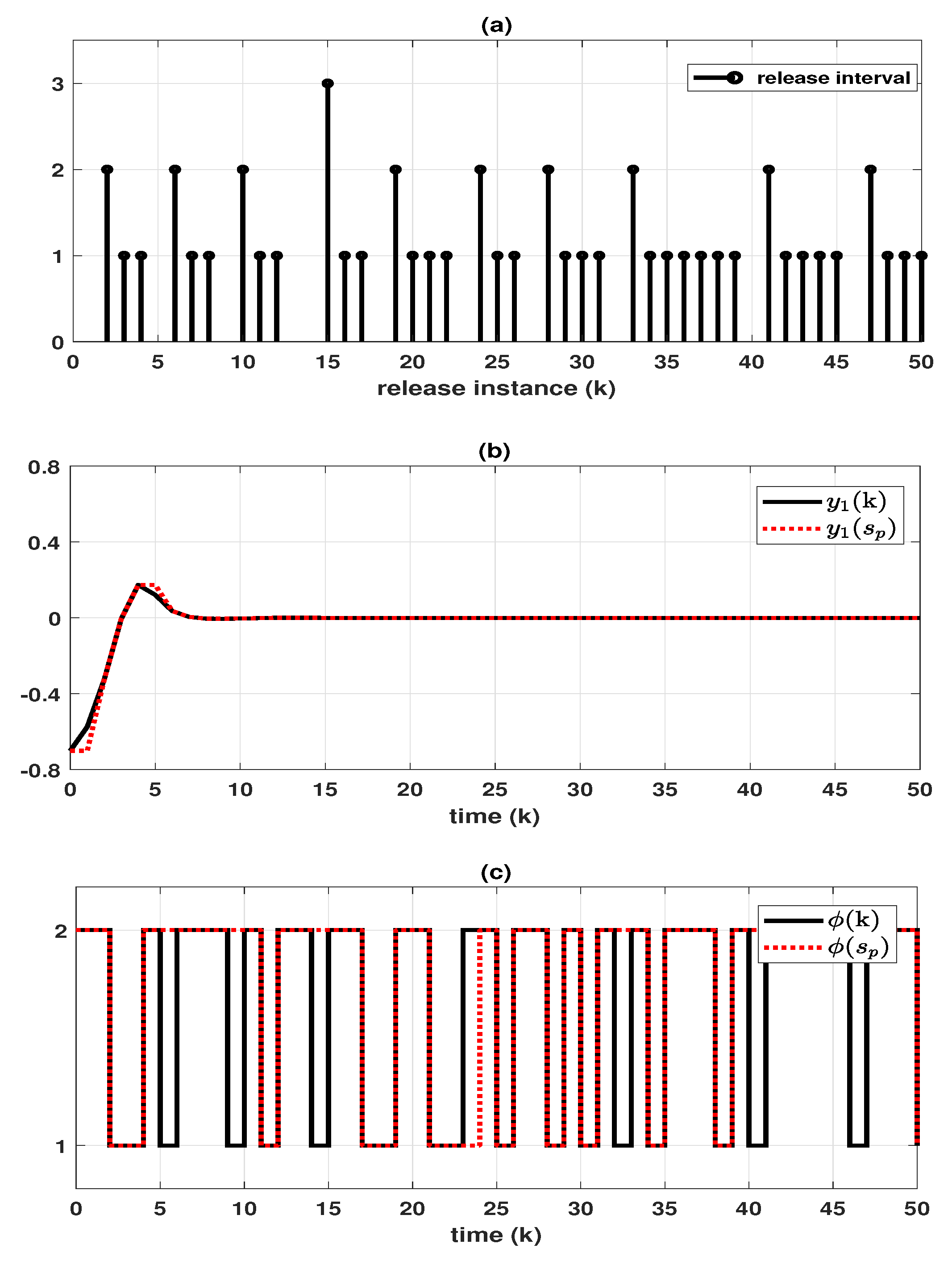
According to the event-triggered scheme, Figure 2a shows the instance when the event generator outputs an ENT signal to the transmitter, then the measured output signal $y\left(k\right)$ and evolution of system mode $\varphi \left(k\right)$ are transmitted to the filter, which are displayed in Figure 2b and Figure 2c, respectively. Especially, since matched error $\delta \left(k\right)\equiv 0$, FBF module constructs the event-triggered fuzzy basis functions ${\theta }_i$ from the measured output $y\left(k\right)$. Based on the obtained non-PDC fuzzy filter gains, Figure 3a,b show the response of $z\left(k\right)$, $\tilde{z}\left(k\right)$, and $\overline{z}\left(k\right)$ for $x\left(0\right)=[-0.8,-0.7]$, $w\left(k\right)\equiv 0$; and Figure 3c,d show the response of $z\left(k\right)$, $\tilde{z}\left(k\right)$, and $\overline{z}\left(k\right)$ for $x\left(0\right)\equiv 0$, $w\left(k\right)=0.5(\mathrm{for}20\le k<25)$, and $w\left(k\right)=0$ (elsewhere). As a result, from Figure 3b, it can be found that the filtering errors converge to zero as time increases, and from Figure 3d, it can be verified that the dissipativity performance $\beta =3.5569$ in Table 2 holds because ${\sum }_{k=0}^T\mathcal{W}\left(k\right)/\beta {\sum }_{k=0}^T{\parallel w\left(k\right)\parallel }^2>1$ is satisfied.

Example 2

(for ${\tilde{\mathbb{H}}}_g\ne Ø$ and $\delta \left(k\right)\ne 0$). Let us consider a tunnel diode circuit system expressed as FMJS with $\varphi \left(k\right)\in {\mathbb{N}}_{\alpha }=\{1,2\}$, adopted in [34]:

$$\begin{array}{cc}\hfill & A_{11}=\left[\begin{array}{cc}0.9987& 0.9024\\ -0.0180& 0.8100\end{array}\right],A_{21}=\left[\begin{array}{cc}0.9980& 1.0000\\ -0.0200& 0.9800\end{array}\right],\hfill \\ \hfill & A_{12}=\left[\begin{array}{cc}0.9034& 0.8617\\ -0.0172& 0.8103\end{array}\right],A_{22}=\left[\begin{array}{cc}0.9080& 1.0000\\ -0.0200& 0.9800\end{array}\right],\hfill \\ \hfill & B_{11}={\left[\begin{array}{cc}0.0093& 0.0181\end{array}\right]}^T,B_{21}={\left[\begin{array}{cc}0.0000& 0.0200\end{array}\right]}^T,\hfill \\ \hfill & B_{12}={\left[\begin{array}{cc}0.0091& 0.0181\end{array}\right]}^T,B_{22}={\left[\begin{array}{cc}0.0000& 0.0200\end{array}\right]}^T,\hfill \\ \hfill & C_{gi}=\left[\begin{array}{cc}1.0& 0.0\\ 0.3& 1.2\end{array}\right],D_{gi}={\left[\begin{array}{cc}0& 1\end{array}\right]}^T,E_{gi}=\left[\begin{array}{cc}1.0& -0.5\end{array}\right],\hfill \end{array}$$

where the fuzzy basis functions are given as

$$\begin{array}{c}\hfill {\theta }_1=\left\{\begin{array}{cc}(3+x_1\left(k\right))/3,\hfill & -3<x_1\left(k\right)\le 0\hfill \\ (3-x_1\left(k\right))/3,\hfill & 0<x_1\left(k\right)<3\hfill \\ 0,\hfill & elsewhere\hfill \end{array}\right.,{\theta }_2=1-{\theta }_1.\end{array}$$

In addition, the transition rates are given as follows:

$$\begin{array}{cc}\hfill & {\left[{\tilde{\pi }}_{gh}\right]}_{g,h\in {\mathbb{N}}_{\alpha }}=\left[\begin{array}{cc}0.6& 0.4\\ 0.7& 0.3\end{array}\right],{\overline{ϵ}}_{gh}=0.1,\forall g,h\in {\mathbb{N}}_{\alpha },\hfill \end{array}$$

which means that ${\mathbb{H}}_1=Ø$, ${\tilde{\mathbb{H}}}_1=\{1,2\}$, ${\mathbb{H}}_2=Ø$, and ${\tilde{\mathbb{H}}}_2=\{1,2\}$. Furthermore, to obtain the simulation results for both synchronous and asynchronous cases, the conditional probabilities are established as follows:

$$\begin{array}{cc}\hfill & Case 1:{\left[{\varpi }_{g\ell }\right]}_{g,\ell \in {\mathbb{N}}_{\alpha }}=\left[\begin{array}{cc}1.0& 0.0\\ 0.0& 1.0\end{array}\right],\hfill \\ \hfill & Case 2:{\left[{\varpi }_{g\ell }\right]}_{g,\ell \in {\mathbb{N}}_{\alpha }}=\left[\begin{array}{cc}0.8& 0.2\\ 0.3& 0.7\end{array}\right].\hfill \end{array}$$

For ${\Gamma }_g=\mathbf{diag}(0.35,0.65)$ and $n_{\tilde{x}}=2$,

Table 3. Comparison of dissipativity performance $\beta$ for different ${\overline{\delta }}_i$.

$\mathit{\beta }$	${\overline{\mathit{\delta }}}_{\mathit{i}}=0$ (Matched)	${\overline{\mathit{\delta }}}_{\mathit{i}}=0.2$	${\overline{\mathit{\delta }}}_{\mathit{i}}=1$
Case 1 (synchronous)	3.3799	3.3297	3.3073
Case 2 (asynchronous)	3.2309	3.2130	3.2119

shows the maximum dissipativity performance level $\beta$ for several ${\overline{\delta }}_i$, obtained by Theorem 1, where $\mathcal{Q}=-0.4$, $\mathcal{S}=-1$, $\mathcal{R}=5$. From Table 3, it can be found that (1) the dissipativity performance deteriorates as the mismatch threshold ${\overline{\delta }}_i$ increase, (2) the synchronous case offers better performance than the asynchronous case.

Meanwhile, for Case 2 and ${\overline{\delta }}_i=0.2$, Theorem 1 offers the following solution:

$$\begin{array}{cc}\hfill & U_{11}^{\left(3\right)}=\left[\begin{array}{cc}2.9531& 4.1538\\ 3.9154& 305.9807\end{array}\right],U_{21}^{\left(3\right)}=\left[\begin{array}{cc}2.9648& 4.4021\\ 3.9404& 299.7105\end{array}\right],\hfill \\ \hfill & U_{12}^{\left(3\right)}=\left[\begin{array}{cc}2.9255& 4.3274\\ 4.3018& 297.8675\end{array}\right],U_{22}^{\left(3\right)}=\left[\begin{array}{cc}2.9524& 4.6780\\ 4.2959& 297.0513\end{array}\right],\hfill \\ \hfill & {\breve{F}}_{11}=\left[\begin{array}{cc}1.2050& 4.2356\\ -3.4986& 266.3810\end{array}\right],{\breve{F}}_{21}=\left[\begin{array}{cc}1.9449& 4.6970\\ -3.7557& 272.5151\end{array}\right],\hfill \\ \hfill & {\breve{F}}_{12}=\left[\begin{array}{cc}1.2157& 4.5272\\ -3.8214& 258.9970\end{array}\right],{\breve{F}}_{22}=\left[\begin{array}{cc}1.8759& 4.9323\\ -3.6577& 267.9507\end{array}\right],\hfill \\ \hfill & {\breve{G}}_{11}=\left[\begin{array}{cc}-1.3113& -0.8770\\ -0.9965& -4.7163\end{array}\right],{\breve{G}}_{21}=\left[\begin{array}{cc}-0.4479& -1.0194\\ -0.3818& -4.5004\end{array}\right],\hfill \\ \hfill & {\breve{G}}_{12}=\left[\begin{array}{cc}-1.2679& -0.8848\\ -2.0525& -4.3402\end{array}\right],{\breve{G}}_{22}=\left[\begin{array}{cc}-0.5171& -0.9728\\ -0.4959& -4.8694\end{array}\right],\hfill \\ \hfill & H_{11}=\left[\begin{array}{cc}-1.3973& -2.4358\end{array}\right],H_{21}=\left[\begin{array}{cc}-1.3395& -3.4061\end{array}\right],\hfill \\ \hfill & H_{12}=\left[\begin{array}{cc}-1.3948& -2.3703\end{array}\right],H_{22}=\left[\begin{array}{cc}-1.3452& -3.6414\end{array}\right],\hfill \\ \hfill & S_{11}=\left[\begin{array}{cc}1.1241& 0.2488\\ 0.2488& 0.7182\end{array}\right],S_{21}=\left[\begin{array}{cc}0.3028& 0.1642\\ 0.1642& 0.9900\end{array}\right],\hfill \\ \hfill & S_{12}=\left[\begin{array}{cc}1.1848& 0.5140\\ 0.5140& 0.7407\end{array}\right],S_{22}=\left[\begin{array}{cc}0.8841& 0.2696\\ 0.2696& 0.8175\end{array}\right].\hfill \end{array}$$

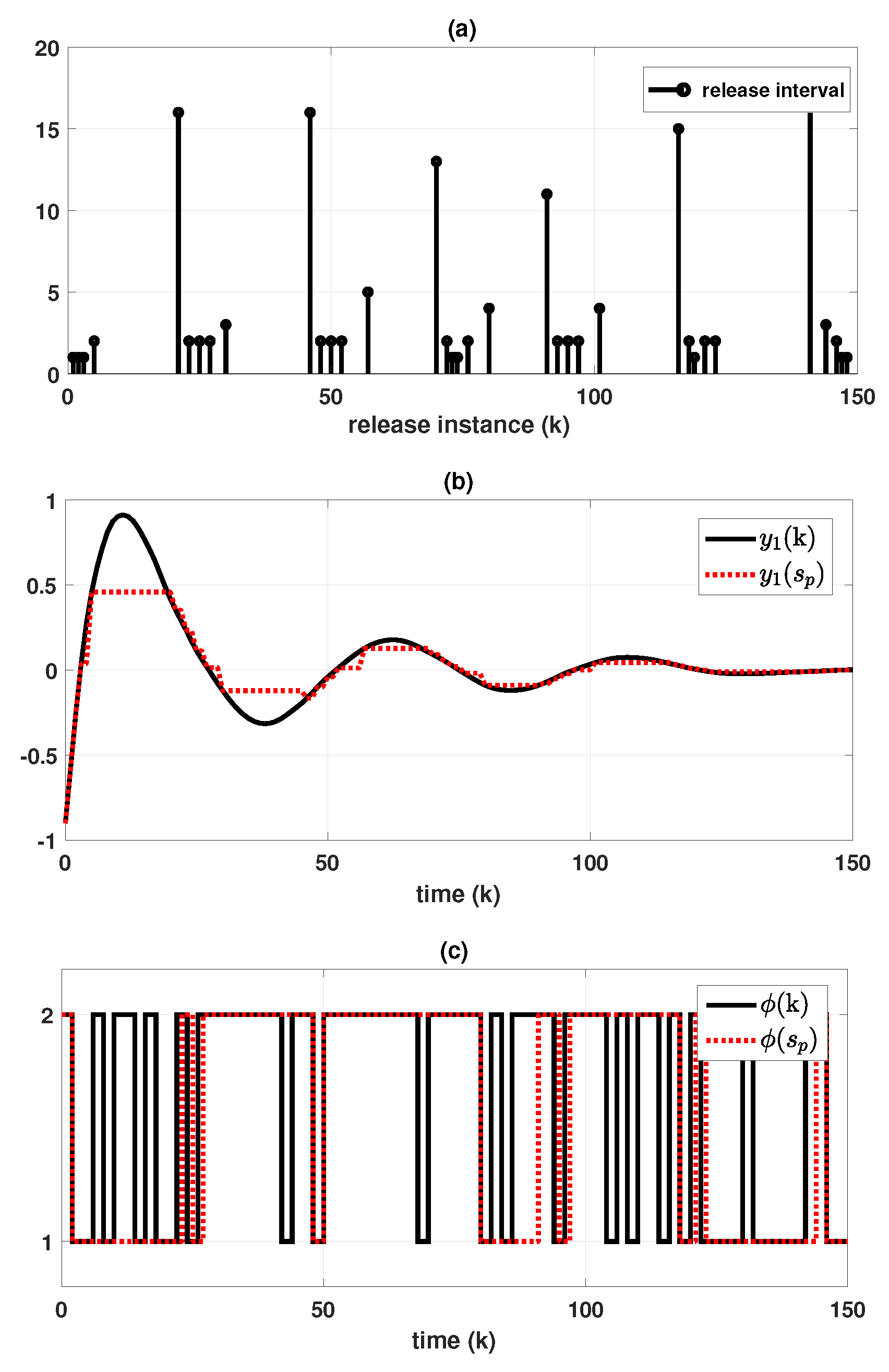
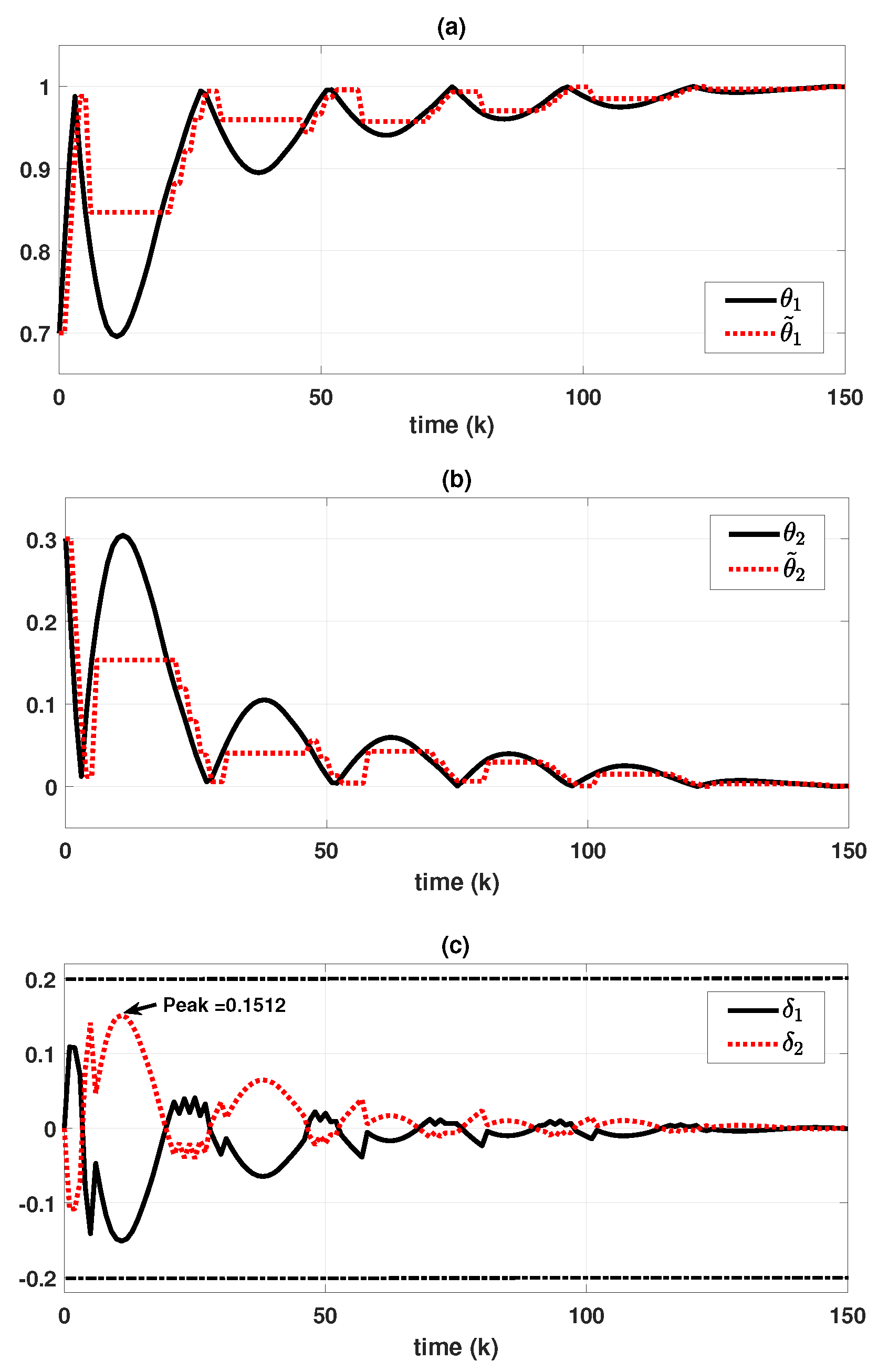
According to the event-triggered scheme, Figure 4a shows the instance when the event generator outputs an ENT signal to the transmitter, then the measured output signal $y\left(k\right)$ and evolution of system mode $\varphi \left(k\right)$ are transmitted to the filter, which are displayed in Figure 4b and Figure 4c, respectively. 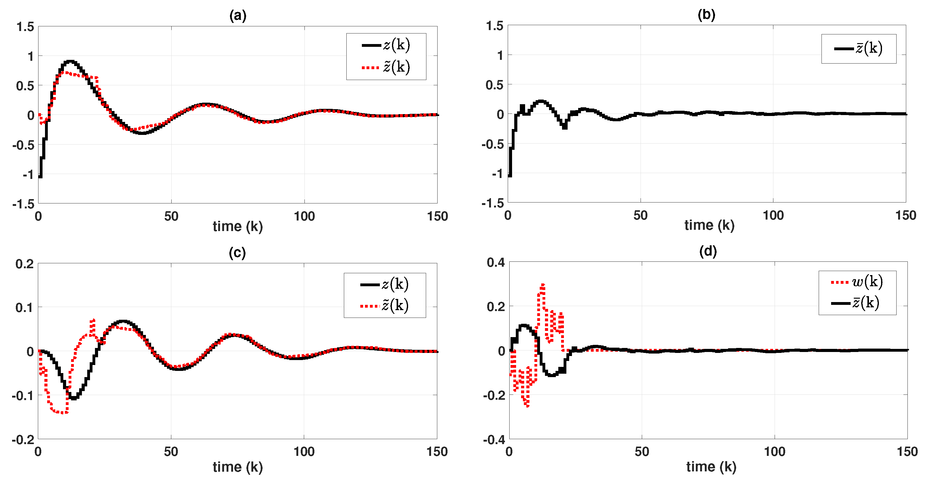From the transmitted output $y\left(s_p\right)$, FBF module constructs the event-triggered fuzzy basis functions ${\tilde{\theta }}_i$, which are shown in Figure 5a,b, and the dynamic behavior of ${\delta }_i={\theta }_i-{\tilde{\theta }}_i$ are presented in Figure 5c. Based on the obtained non-PDC fuzzy filter gains, Figure 6a,b show the response of $z\left(k\right)$, $\tilde{z}\left(k\right)$, and $\overline{z}\left(k\right)$ for $x\left(0\right)=[-0.9,0.3]$, $w\left(k\right)\equiv 0$; and Figure 6c,d show the response of $z\left(k\right)$, $\tilde{z}\left(k\right)$, and $\overline{z}\left(k\right)$ for zero initial $x\left(0\right)\equiv 0$, $w\left(k\right)=-0.5\times \mathrm{rand}[0,1](\mathrm{for}1\le k\le 10)$, $w\left(k\right)=0.5\times \mathrm{rand}[0,1](\mathrm{for}11\le k\le 20)$, and $w\left(k\right)=0$(elsewhere). As a result, from Figure 6b, it can be found that the filtering errors converge to zero as time increases, and from Figure 6d, it can be seen that the dissipativity performance $\beta =3.2130$ in Table 3 holds because ${\sum }_{k=0}^T\mathcal{W}\left(k\right)/\beta {\sum }_{k=0}^T{\parallel w\left(k\right)\parallel }^2>1$ is satisfied. Not only that, it can be verified from Figure 5c that ${\delta }_i$ satisfies $|{\delta }_i|\le 0.1512<{\overline{\delta }}_i=0.2$, for $i\in {\mathbb{N}}_r$.

5. Concluding Remarks

In this paper, we have studied the event-triggered dissipative filtering problem of nonhomogeneous FMJSs against asynchronous modes and mismatched premise variables. To sum up, the proposed method makes significant progress in improving the filter performance (i) by using a non-PDC scheme for the construction of asynchronous mode-dependent fuzzy filter gains, (ii) by making the event generation function dependent on fuzzy basis functions, and (iii) by implementing a relaxation processes that takes advantage of stringent constraints on time-varying paraemters.