
The Kinematics of a Bipod R2RR Coupling between Two Non-Coplanar Shafts
by
 ,
,
Stelian Alaci
1,*, 
Ioan Doroftei
2,
Florina-Carmen Ciornei
1,
Ionut-Cristian Romanu
1 and
Ioan Alexandru Doroftei
2 1
Faculty of Mechanics, Automotive and Robotics, Stefan cel Mare University of Suceava, 720229 Suceava, Romania
2
Mechanical Engineering Faculty, Gheorghe Asachi Technical University of Iasi, 700050 Iasi, Romania
*
Author to whom correspondence should be addressed.
Mathematics 2022, 10(16), 2898; https://doi.org/10.3390/math10162898
Submission received: 10 June 2022
/
Revised: 7 August 2022
/
Accepted: 10 August 2022
/
Published: 12 August 2022
(This article belongs to the Topic Engineering Mathematics)
Abstract
:The paper presents a new solution for motion transmission between two shafts with non-intersecting axes. The structural considerations fundament the existence in the structure of the mechanism of three revolute pairs and a bipod contact. Compared to classical solutions, where linkages with cylindrical pairs are used, our solution proposes a kinematical chain also containing higher pairs. Due to the presence of a higher pair, the transmission is much simpler, the number of elements decreases, and as a consequence, the kinematical study is straightforward. Regardless, the classical analysis of linkages cannot be applied because of the presence of the higher pair. For the proposed spatial coupling, the transmission ratio is expressed as a function of constructive parameters. The positional analysis of the mechanism cannot be performed using the Hartenberg–Denavit method due to the presence of a bipod contact, and instead, the geometrical conditions of existence for the bipod contact are applied. The Hartenberg–Denavit method requires the replacement of the bipodic coupling with a kinematic linkage with cylindrical (revolute and prismatic) pairs, resulting in complicated analytical calculus. To avoid this aspect, the geometrical conditions required by the bipod coupling were expressed in vector form, and thus, the calculus is significantly reduced. The kinematical solution for the proposed transmission can be obtained in two ways: first, by considering the equivalent transmission containing only cylindrical pairs and applying the classical analysis methods; second, by directly expressing the condition of definition for the higher pairs (bipodic pair) in vector form. The last method arrives at a simpler solution for which analytical relations for the positional parameters are obtained, with one exception where numerical calculus is needed (but the precision of this parameter is controlled). The analytical kinematics results show two possibilities of building the actual mechanism with the same constructive parameters. The rotation motions from the revolute pairs, internal and driven, and the motions from the bipod joint were obtained through numerical methods since the equations are very intricate and cannot be solved analytically. The excellent agreement validates the theoretical solutions obtained and the possibility of applying such mechanisms in technical applications. The constructive solution exemplified here is simple and robust.
MSC:
70B15; 70Q051. Introduction
The transmission of motion is a classical—but also modern—issue [1] with applications to cutting-edge systems, such as medical robots [2], bioinspired robots [3], and hybrid robotic systems [4], where the problem of motion control of the effector element [5,6] is always a key task. There are solutions with classical couplings constructed with rigid elements but also solutions of extreme novelty, such as compliant couplings [7,8,9,10,11].
From a constructive point of view, the single pair that is suitable to be designed with compliant elements is the intermediate revolute pair. This pair can be used for reduced stress and low angular speed, otherwise the risk of vibrations occurrence due to elastic elements will appear. Compliant mechanisms have some limitations, such as complicated design calculus, difficulty of controlling the deformation, and lack of precision. They also raise problems such as fatigue strength and efficiency due to the fact that the elastic elements store and dissipate energy.
Because the mechanism is spatial, the loading of the elastic element is complex and conducts difficult-to-control behavior. In addition to the difficult design of the compliant mechanism, the special and complex construction, difficult assemblage, and more complicated running and maintenance are some aspects to be mentioned when classical and compliant couplings are balanced. We must also consider that the compliant couplings are dedicated to small torques and the strains must be kept within the elastic domain, or else the plastic deformations occur. They cannot transmit continuous rotation motion. The costs of compliant mechanisms are obviously greater than those for classical couplings constructed with rigid elements. A rigorous study is very complex, and simplified models are demanded, such as a pseudo-rigid-body model [12,13].
In 2015, D. Farhadi Machekposhyi [7] realized a comparative analysis between spatial couplings with rigid elements versus compliant couplings, but in this analysis, no spatial coupling with four rigid elements is mentioned. In current illustrations, the solid bodies constituting a system interrelate to each other [14] with the final goal that the system fulfils the function for which it was designed. In a first approximation, each of the constitutive elements of a mechanical system can be regarded as a rigid body called a kinematic element and having six degrees of freedom: three rotations and three translations. Connecting several elements in a system, the degree of freedom of the system increases to , where is the total number of elements of the system. However, in order to accomplish the function of the system, it is required that the elements of the system interact with each other, and this leads to a decrease in the degrees of freedom.
The analysis of the mobility of a system is based on fundamental concepts, from which a kinematical pair that is a direct, mobile, and permanent connection between two kinematic elements is obtained. The foremost classification criterion of the kinematic pairs is the class, defined as the number of degrees of freedom withdrawn from an element when the other element is considered immobile. Based on this definition, the class of kinematic pair may have values between 1 and 5. By extrapolating the definition, one considers the pair of class as the pair corresponding to the lack of interaction between two elements and the pair of class characteristic to the rigid link between two elements. All the elements of the system linked to each other by kinematic pairs create a kinematic chain characterized by the degree of freedom (DOF) [15]:
Equation (1) shows that in order to ensure a well-defined motion of the entire kinematic chain, control of all the L degrees of freedom is required. Two situations are met in practical applications: the open chain, in which, in the structure of the chain, at least one element exists which makes a single pair, as seen in robotic structures and the closed chain, in which each element creates at least two kinematic pairs, characteristic to mechanisms. In order to calculate the degree of mobility of a mechanism, it is considered that one of the elements is immobile and the motions of all other elements are considered relative to this fixed element [16,17]:
A frequent problem in mechanical engineering is the transmission of rotation motion between two shafts with non-coplanar axes. A usual engine provides the rotation motion of the driving shaft, and, for many situations, this is a uniform rotation motion. The parameter describing the quality of transmission of motion is the transmission ratio:
where is the angular velocity of the driving shaft and is the angular velocity of the driven shaft. For a transmission ratio equal to one, a special case of transmission known as homokinetic transmission materializes. Diverse solutions of homokinetic couplings are presented in technical literature [18,19,20,21,22,23,24,25]. There is also a wide range of applications in which the rigorously constant transmission ratio is not necessary and in which it is accepted that the transmission ratio may have a periodic variation about a mean value, with stipulated deviation between accepted limits [26]. One of the aspects occurring in the case of motion transmission between two shafts is the presence of sliding friction existing in the kinematic pairs from the kinematic chain, a fact that reduces the efficiency of transmission [27,28]. This happens in the cases when the transmission of motion is completed using a small number of elements—such as direct contact between the input and output elements or with an intermediate element between them. The structural calculus reveals that for these cases, between the elements of the coupling kinematic chain, pairs of lower class will exist (, , and planar joint) which cannot be envisaged for rolling friction [29,30]. The requirement of optimum design assumes a structural solution as simple as possible for ensuring a higher efficiency. The necessity of quantitative evaluation of the manner in which the motion is transmitted from driving shaft (1) to the driven shaft () demands that the transmission ratio be expressed as a function of the constructive characteristics of the mechanism.
For planar mechanisms, an efficient method is the vector loop method [17,31,32], which expresses the condition of a closed contour of the kinematic chains of the mechanism in vector or complex form. The kinematic analysis of spatial mechanisms can be performed via different analytic methods based on the kinematical closed chain of the mechanisms, such as dual quaternions [33], the screw method, the bar method, the method of homogeneous operators, the matrix–tensor method, or the matrix invariants method [34].
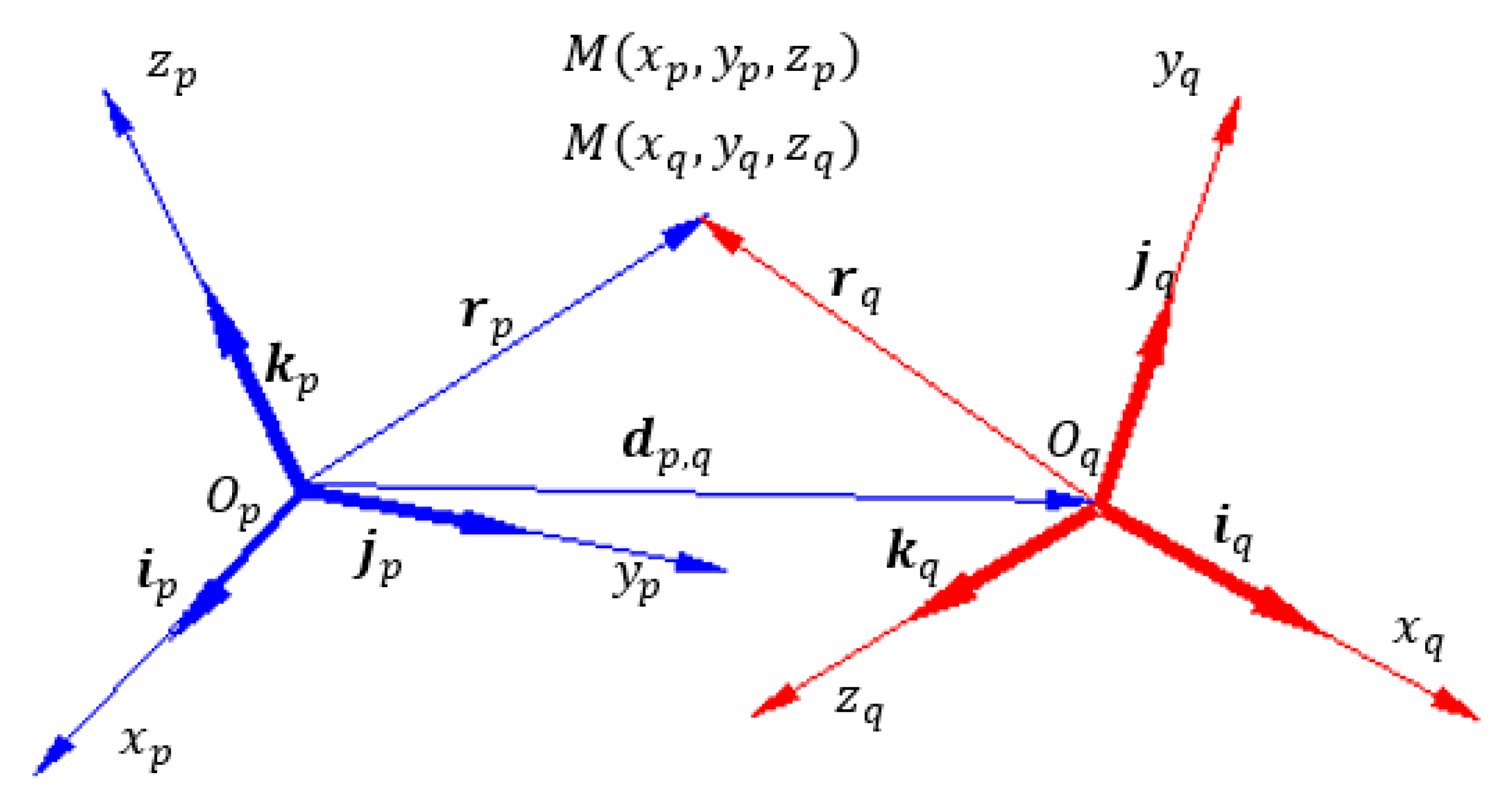
The kinematic analysis of the mechanism presented in the present paper is based on the homogeneous operators method, which was proposed by Hartenberg and Denavit [35]. The method created by Hartenberg and Denavit became classical, but it continues to be applied to the kinematic study [36,37,38,39] of most recent systems, such as spatial mechanisms and robots [40,41,42,43,44,45,46]. There is no specified methodology for the kinematic analysis of the mechanisms with higher pairs. If a stated methodology is to be applied, it is required that all the kinematical higher pairs must be replaced by kinematical chains that have only cylindrical pairs (with particular forms revolute and translational) in their structures. From the known methodologies, one can mention the Hartenberg–Denavit method of dual operators [47,48], the screw method [49], and the method of dual quaternions [50]. In the paper, a general method is applied [51,52,53,54,55] that is appropriate to any type of spatial mechanism. The method is based on the relation of coordinate transformation of a point when the reference system is changed. The point M, Figure 1, has in two coordinate systems p and q the position vectors and , respectively. By denoting with the versors of the p system and by the versors of the q system, the coordinate transformation is expressed in matrix form, and the passing from the p system to q system is described by a rotation matrix :
and a displacement vector , characterizing the displacement of the origin of the p system over the origin of the q system:
The transformation relation is:
McCarthy [56,57] gives an especially interesting remark, considering the coordinate transformation (6) as a displacement from the initial position “p” to a final position “q”. Since the two versor systems and are orthonormal coordinate systems, from the nine elements of the matrix, only three are independent. One can conclude that the relative position of the two systems is described by six scalar parameters. Due to the nonhomogeneous character of Relation (6), applying the relation successively leads to intricate relations. Hartenberg and Denavit proposed the writing the relation in the following form:
Equation (7) can be regarded as a gliding in the hyper plane from the four-dimensional space where the displacement is described by the homogeneous operator:
Relation (8) presents an important consequence: when attaching a coordinate system to each element of the chain, the coordinates of a point, after successive passes through all coordinate systems, will be the same after returning to the initial frame. For a given closed kinematic chain of n elements, when the convention that the element denoted n + 1 is identical to element 1, the vector loop equation is written:
where is the unit matrix of order 4. Equation (9) provides 12 scalar equations, of which six are independent, and the position of the kinematic chain can thus be found. The system of scalar equations is a nonlinear one, with multiple solutions corresponding to all assembling possibilities. Uicker [17] presents a numerical method for solving the system of scalar equations. A generalized method for any kinematics chain type, closed or open, is presented by [58]. The papers [59,60,61,62] present a review of spatial couplings with constant velocity. Four-element coupling does not occur; only coupling with five or more elements exists. Regarding the spatial mechanisms, the kinematical analysis can be performed using the Hartenberg–Denavit method only if, as emphasized in the paper, in the structure of the mechanism only cylindrical pairs (represented in Figure 2) occur (possible with particular forms: prismatic, revolute, and helical joint). For other types of mechanisms (in this case as well), the replacement of non-cylindrical pairs with kinematical chains in which only cylindrical pairs occur (with the particular forms) is required. For example, Fisher [63] presents the manner of applying the Hartenberg–Denavit method in dual form for the mechanisms containing spherical pairs and planar joints. The attempt to find mechanisms with four elements with higher pairs on the internet did not produce a result. From the category of spatial mechanisms with higher pairs, the most representative examples are the spatial cam mechanisms [59,60,61,62,64,65,66,67].
Another example: in 2011, Bil studied the spatial mechanism with higher pairs [66,67] by means of the fundamental equivalent mechanism 7R. The importance of the subject is reflected by classical monographs [20,68,69,70].
In order to apply the Hartenberg–Denavit method, the axis z will be represented by the axis of the prismatic joints and the axis x will be represented by the common normals of two successive z axes, as shown in Figure 3.
Overlaying the system and the system by means of a roto-translation of parameters and along the axis followed by a roto-translation of parameters and around the axis , the homogeneous operator results as a composition of two homogeneous operators, and :
Recalling the remark given by McCarthy, the two matrixes and can be viewed as homogeneous operators that describe roto-translations with respect to the axes and , respectively. Thus, the symbolisation of the axes with two indices appears natural; for example, will now be in order to suggest that the axis is in fact the normal to the axes and . Additionally, the notation with two indices clearly indicates the fact that the axes and are attached to the same element and that the two parameters and are the constructive characteristics of the element.
Seemingly restrictive, due to the imposed condition that only cylindrical joints should occur in the mechanism’s structure, the Hartenberg–Denavit method can be applied to any mechanism, with the condition that all joints different from cylindrical ones be previously equivalated to combinations of cylindrical joints. The proposed method does not present restrictions because any pair is represented by a series of geometrical restrictions that can be expressed in vector form, and after that, using the transformation relations from the Hartenberg–Denavit method, all the vectors can be expressed by their projections on the axes of a unique system of coordinates in order to obtain the scalar equations of projections. The method is exemplified in [71] for the swash plate mechanisms, where the sphere–plane joint of the first class is equivalated to a Cardan coupling in series with an Oldham coupling. The method presents the disadvantage that all the motions from the joints of the equivalent mechanism must be found in order to obtain the motions from the joints of the actual mechanism. In the present work, it will be proven that for the kinematic analysis, it is more efficient to use the condition equation of the kinematic joints (other than cylindrical). In other papers concerning higher pairs, the equations of condition are not used in vector form—which is a simpler form—but in more intricate forms (algebraic, by projections); for illustration, see [72,73,74,75,76]. The condition equations in vector form express the relations existing between different vectors identified in different reference coordinate systems. In order to make these equations operable, it is required that all the vectors be identified in the same coordinate system; therefore, the transformation relations from the homogeneous operators method are applied in a simple manner. The classical method based on the equation of closed contour of the mechanism assumes that the bipodic pair is replaced by an assembly of elements which are linked through kinematical lower pairs. As a result of applying the classical method, an over-constrained system of 12 equations with six unknowns results, and for solving it, in most cases, numerical calculus must be used [77]. As a general conclusion of the above considerations, the kinematical study of a transmission with multipodic contacts cannot be performed via classical methods. In the present paper, a general methodology is proposed with the bipodic contact as example, and it is based on the statement by Phillips [78] that any pair can be assimilated by the relation between the points () of an element with respect to the surface of the other element. To solve the problem, these relations must be expressed in vector form with the mention that all vectors should be expressed in the same reference system.
2. Materials and Methods
2.1. Structural Considerations
Straightforward calculus shows that the unique solution for transmitting the rotation motion by direct contact between two shafts with non-coplanar axes is possible when a pair of class 1 exists between them [79]. In a general case, the transmission of rotation of motion between two shafts with non-coplanar axes can be achieved via a kinematic chain having in structure n elements and pairs of class. As a consequence, the total number of elements of the chain is because to the number of elements of the chain, the two shafts and the ground are added. To the pairs of the chain there must be added 2 pairs of class 5, , which connect to the ground the driving and driven shafts. The mobility of the transmission should be since a single driving element exists. Equation (2) is applied for the coupling mechanism:
The simplest solution is the direct contact, :
from which results
The single possible solution of Equation (13) is
System (14) shows that for two shafts with non-coplanar axes, direct coupling can be achieved only by means of a pair of class obtained through a Hertzian point contact. From the mechanisms that correspond to this category, one can recall hypoid gears, gear mechanisms with intersecting axes, and spatial cam mechanisms. In papers [66,67], there are theoretically modelled different particular aspects concerning higher pairs, but kinematical analysis for each particular solution is not performed.
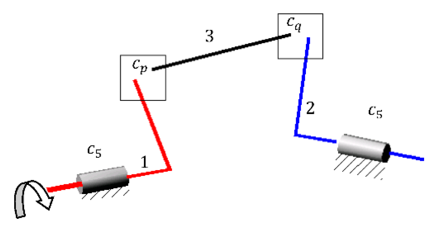
When the coupling is obtained using an intermediate element, as presented in Figure 4, it is considered that the intermediate element makes with each of two shafts a pair of class and , respectively, .
Applying the equation
in this case, from the possible solutions of Equation (2), gives
from which it results
with the possible solutions
and
It deserves mention that the structural solutions obtained by changing the values of the indices and are also valid. One can remark that when the notion of generalized pair of class (non-contacting elements) and (elements rigidly connected) is accepted, the following structural solution can be added to Solutions (18) and (19):
This solution corresponds to the rigid coupling between the intermediate element and one of the shafts, and thus—in fact—it is a direct contact between two shafts, and the motion is transmitted by a direct contact.
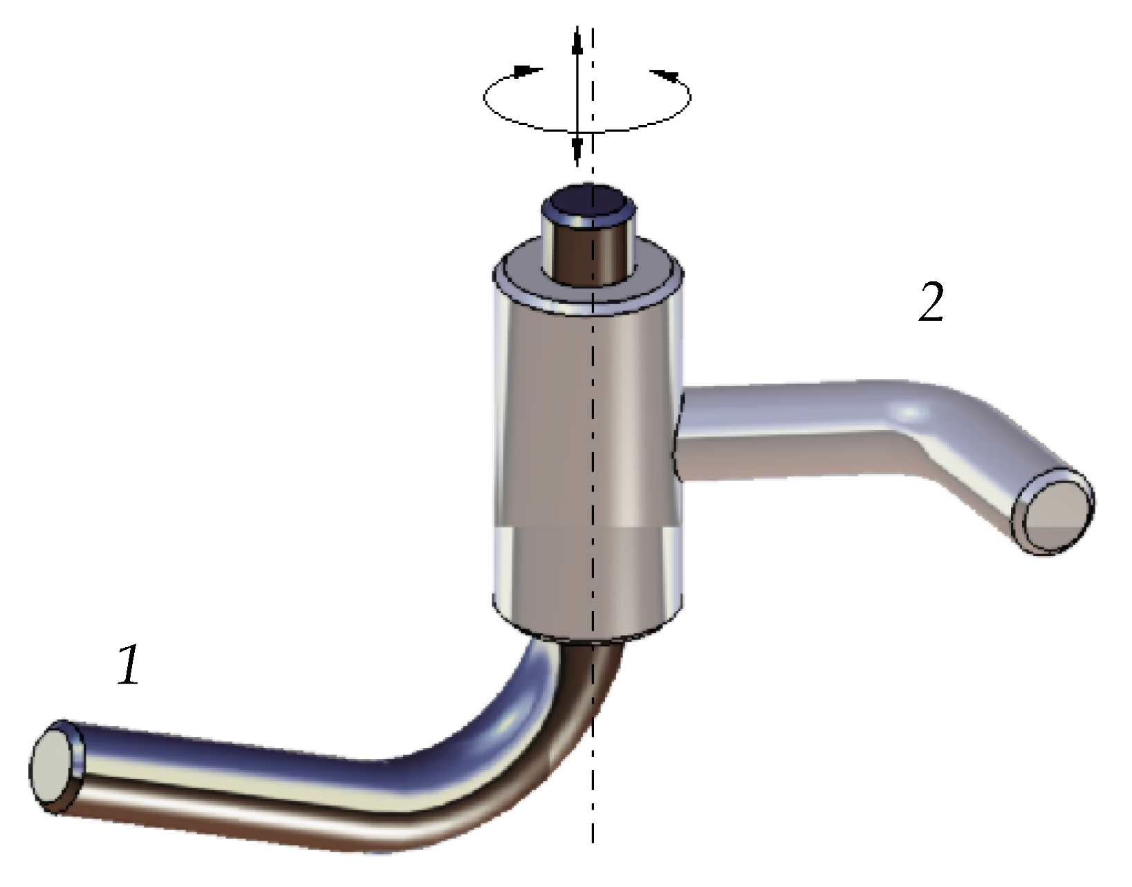
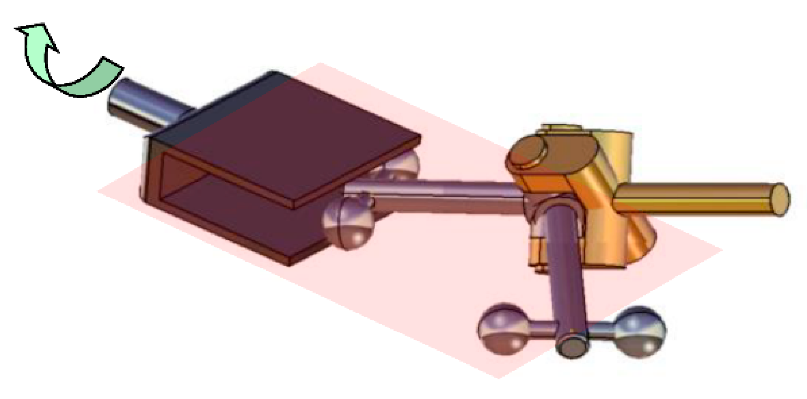
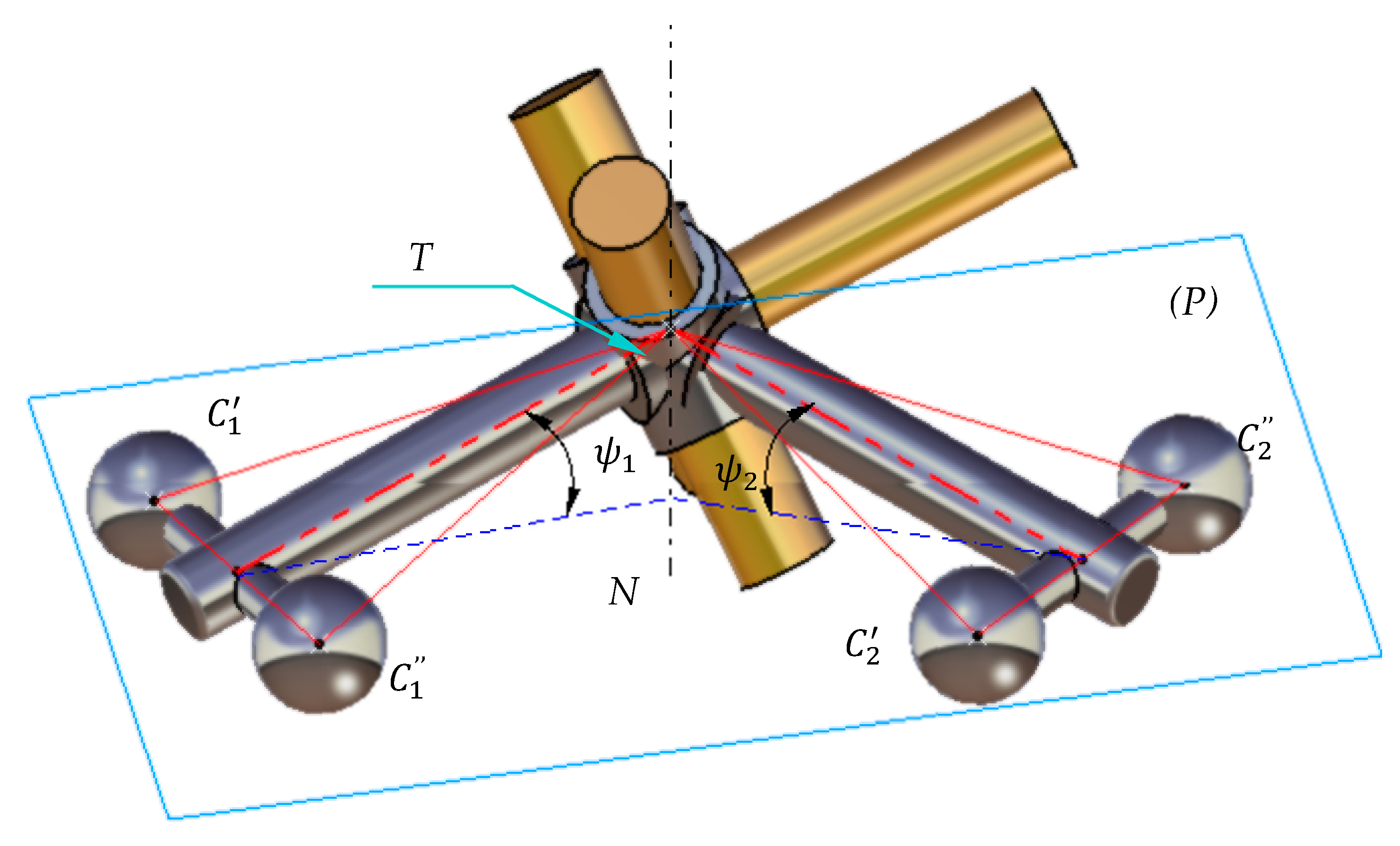
Next, the coupling mechanism where the intermediate elements make a class pair and a class rotation pair with the two shafts, respectively, will be considered. The resulting mechanisms will be R2RR or RR2R mechanisms. The revolute pair is shown in Figure 5, and the bipod joint is presented in Figure 6.
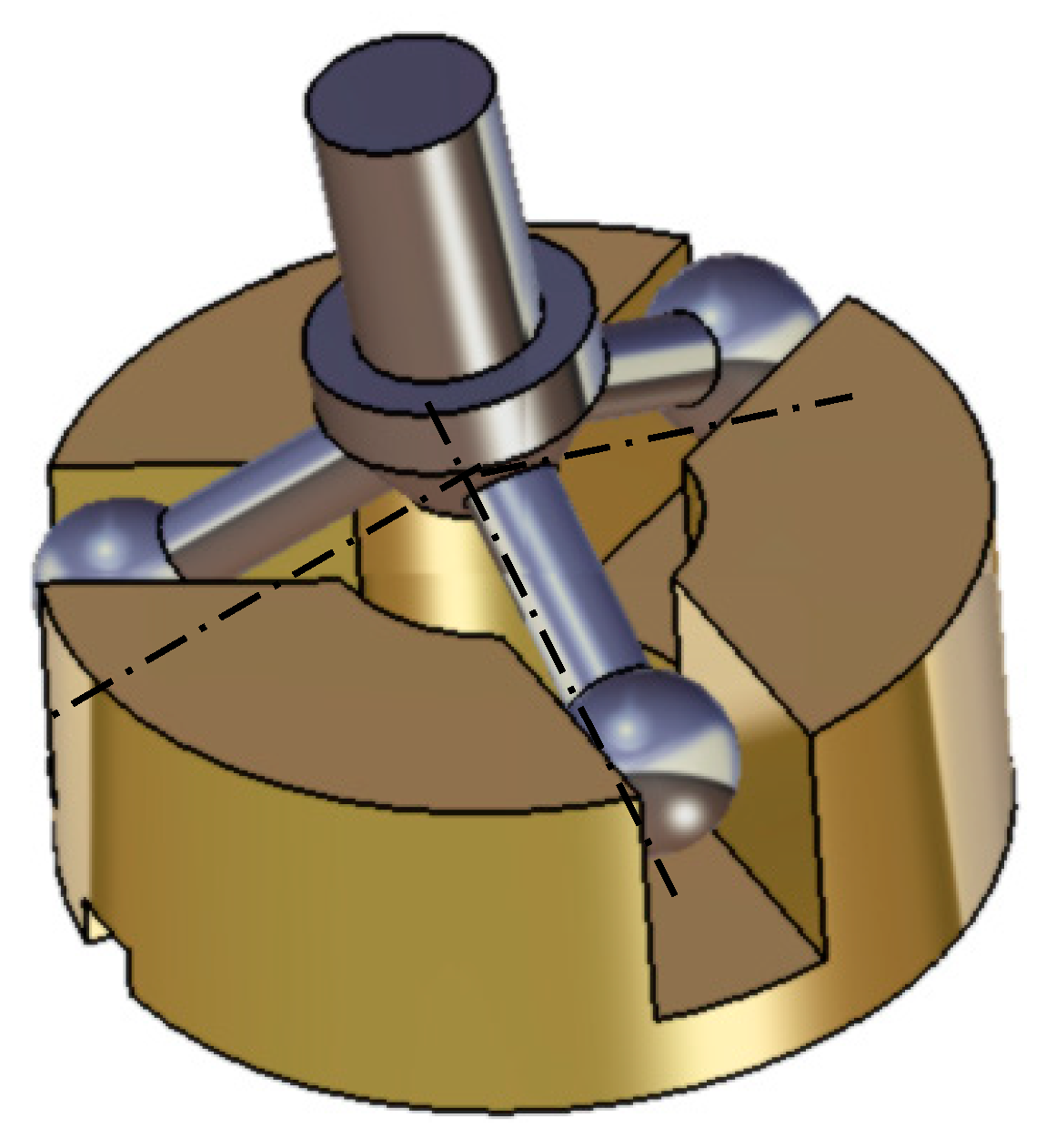
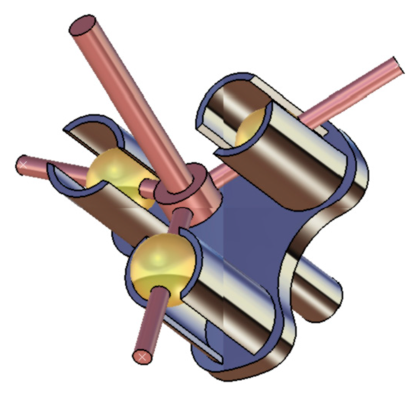
The bipod pair assumes that between the two elements, denoted 1 and 2, two-point concentrated contacts are made. In Figure 6, the two contacts are achieved between spherical surfaces from element 2 and two surfaces attached to element 1. The geometric conditions for the existence of the contacts consist of maintaining the centers of the spheres, and , at distances equal to the radius with respect to the two supporting surfaces and , respectively. In engineering applications, the supporting surfaces are simple surfaces, such as planes, cylinders, etc. A common situation is when the two supporting surfaces are materialized by the same plane and the radii of the two spheres are equal. In this case, the condition of existence for the bipod contact imposes that the axis of the center of spheres is permanently contained in a plane fixed to the other element. The practical solution is presented in Figure 7, in which the balls, attached to the intermediate element, are introduced in a prismatic channel with width equal to the balls’ diameter. Another constructive solution consists of replacing the balls with a metallic cylinder with the same diameter as the balls.
Next, the case , is considered, accepting that class pair is a revolute pair. The mechanism corresponding to this structural solution is presented in Figure 8. The class pair is obtained, in theory, by constraining two points from the intermediate element 3 to lie permanently in a plane attached to element 1. In practice, the class 2 pair is made by introducing two identical spheres attached to the element 3 in a parallelepipedal channel of width equal to the spheres’ diameter, made in the body of element 1. Thus, the centers of the spheres and are permanently constrained to be situated in the plane of symmetry of the channel.
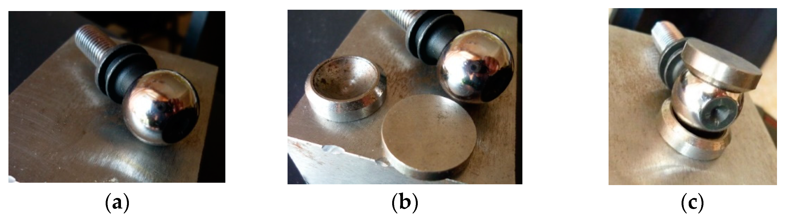
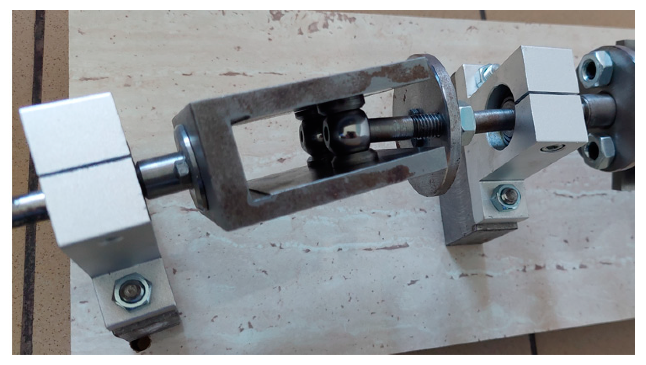
The existence of the sphere–plane contacts, Figure 8 and Figure 9a, which theoretically make the bipod pair, has as its main disadvantage the generation of appreciable contact stresses [80,81]. These stresses may exceed the admissible values, and in consequence, plastic deformations may occur in the materials of the two parts and the actual contact surfaces differ from the theoretical ones. As a practical solution for the transmission, in order to surpass this drawback, Ref. [53] presented the design of an intermediate pad which has a spherical cavity of the same radius as the ball and a flat surface. This pad is introduced between the sphere and the surfaces of the channel to reduce contact stresses, as seen in Figure 9b. The pad and the sphere make a spherical pair, and the pad and the surface of the channel make a planar pair. Both pairs are lower pairs; the contact occurs on extended surfaces, and the effect is the substantial decrease in contact surfaces. Additionally, the tribological behavior of the pad–ball contact and pad–channel contact can be improved by the adequate choice of materials for the pad (bronze, cast iron with nodular graphite, polytetrafluoroethylene PTFE—Teflon, etc.) and by using grease for friction diminishing. In the present case, the pad was made of cast iron with nodular graphite FGN30. For each of the balls, two pads are necessary, and the dimensions of the pad–ball–pad pack are established at assembly—see Figure 9c—because an optimum clearance is required between the pack and the walls of the channel. The constructive solution of the bipod pair is presented in Figure 10.
2.2. Kinematic Analysis of the Mechanism
A first general remark is that for the mechanisms where the sphere–plane contacts are present, due to the great number of degrees of freedom allowed for this pair, kinematic analysis is difficult. From the literature, the affirmation made by Phillips [78] concerning the tripod coupling from Figure 11: “the mechanics of this joint is complicated. It is not well understood” can be mentioned. Another constructive solution based on the curve contact proposed in [72,73] is presented in Figure 12.
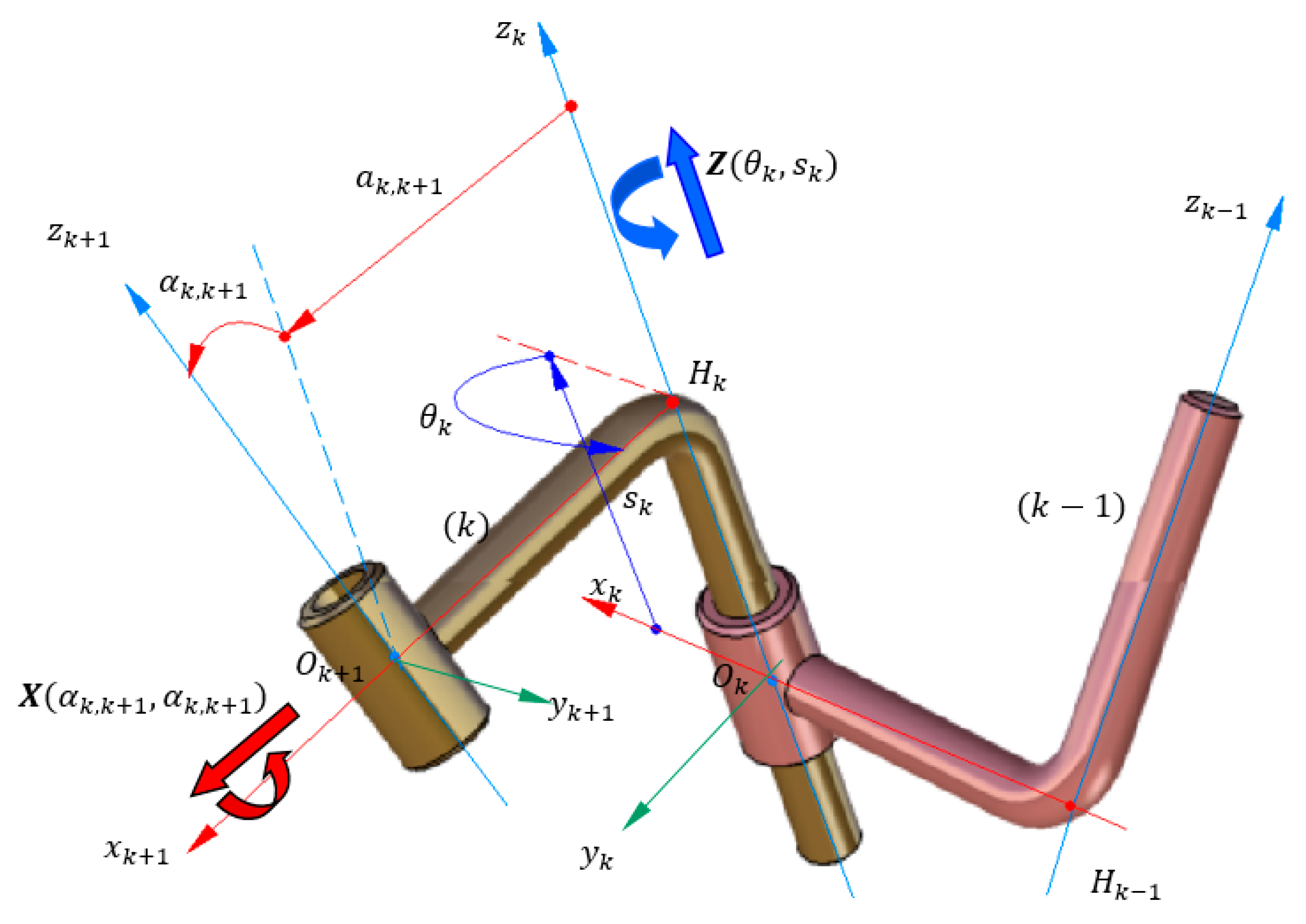
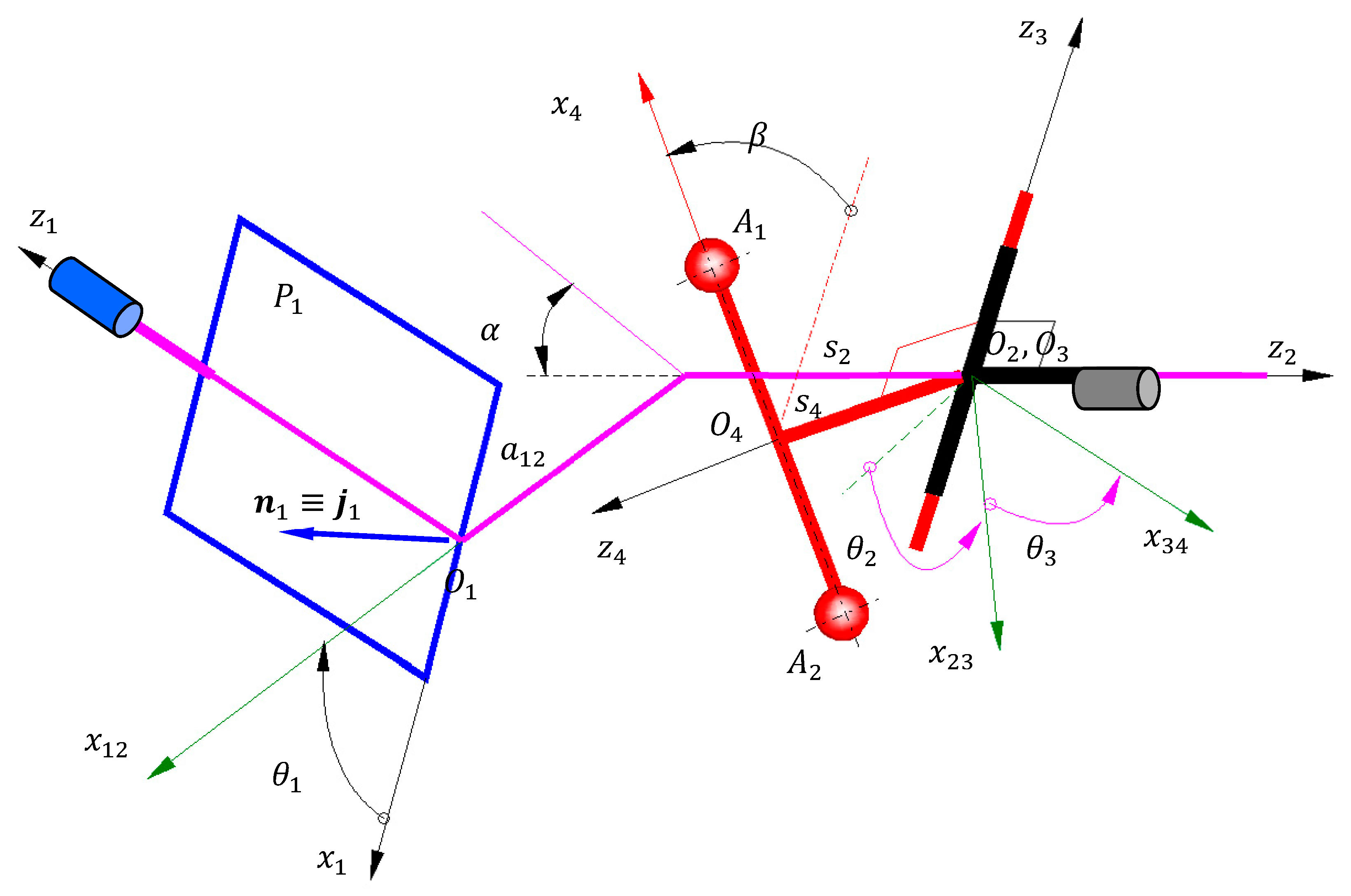
In the present case, the bipod joint presents a greater number of DOF compared to the tripod joint, and therefore, it is expected that the kinematic analysis of the bipod joint should be more complicated than that of the tripod joint, for which a complete analytical solution is presented in [53]. The scheme and the constructive parameters of the mechanisms from Figure 8 are presented in Figure 13. The axes of the rotation pairs are denoted according to the Hartenberg–Denavit [81] convention: is the rotation axis between the ground and the driving element, is the rotation axis between the driven element and the ground, and is the rotation axis between the intermediate and the driven element. The position between the driven and driving elements is specified by the angle and the length of the common normal, . The straight line passing through the centers and is the axis of a coordinate system attached to the intermediate element. The position of this axis is specified with respect to the axis by the rotation and the length of the common normal . The axis has the direction of the common normal of the axes. The axis is fixed to element 1, and it is contained in the plane of symmetry of the channel. For a position of the driving element stipulated by the angle , forcing the points and to lay in the plane the position of the mechanism is completely determined by the rotation angles , from the other two rotation pairs. The origin of coordinate system 1 is denoted , and the condition that the points and belong to the plane is written in vector form:
where is the versor of the normal to the plane which coincides with versor of coordinate system 1. The relations of (21) can be written in the form:
In Relation (22), the vectors and are known by the projections on the axes of system 1, while the vectors are stipulated by the projections on the axes of frame 4. In order to make these equations operable, all vectors must be expressed in the same reference system. To this end, the coordinate transformation relations are used and the Hertenberg–Denavit homogeneous operators method is applied [81]. The notations and are used:
The homogeneous operators correspond to roto-translation with respect to axis z and axis x, respectively. The relation of coordinate transformation from the system 4 to the system 1 is applied based on Figure 13, using the matrix relation:
where:
In the above relations, the convention used is that the vector x is characterized in the coordinate system indicated by the superscript index. From Figure 13, one can notice that:
The problem of how to choose the coordinate system for expressing the vector components from Equation (7) in order to result equations as simpler as possible arises. Aiming to solve that problem, a reference system is chosen denoted generically by from the succession of frames met in the product that defines the operator . The matrix form of the relations (7) expressed in the coordinate system is:
or, in explicit manner,
Equation (30) can be written as:
After the calculus from Equation (31) is performed, it results in
With the aid of the relation
Equation (32) takes the form:
where matrix is the unit matrix of fourth order and the final form of Relation (34) is:
It is remarked that the form of Equation (21) does not depend on the index q—that is, it is independent of the reference frame in which the equations of condition of the pair of second class are expressed. From here, the conclusion that the scalar form of Equation (7) does not depend on the reference coordinate system in which the vectors are expressed. In order to obtain the concrete scalar form of Equation (7), in Relations (35), the following relations are considered:
In Relation (37), are the abscissas of the centers of the balls in reference coordinate system 4. Considering Relations (37) and (35), after calculus is performed, two complicated relations result. However, it is noticed that by adding and subtracting the two scalar equations, two simpler scalar equations are obtained. These equations express the conditions that the sum and the difference of the vectors and are placed in the plane of symmetry of the channel made in the driving element:
The unknowns of the trigonometrical system (38) are the angles and , which obviously depend on the rotation angle of the driving element, . Because the system of Equation (38) is a non-algebraic one, it is expected that it has more solutions corresponding to the assemblage possibilities of the mechanism for a given position of the driving element. Theoretically, System (38) can be solved, and the solution is expressed using the common trigonometrical functions of a single argument. The disadvantage of using trigonometrical functions of unique argument—, , and —is the fact that they have the co-domain of length while the variations of the motions from the mechanisms’ joints may extend to . Thus, there is the risk that the solutions of System (38) given by inverse trigonometrical functions by a unique argument do not correspond to physical reality. To overcome this aspect, the inverse trigonometrical functions of two arguments [82,83] that have the extent of the co-domain , must be used: , , . To this purpose, one can remark that the system is linear with respect to and or and . As example, the system is solved by considering and as the unknowns and it results in:
By writing
an equation is obtained, written in the form
where the function depends on the variable and the parameter . The solution of Equation (41) has the form
Next, the angle is obtained by replacing the values of given by Equation (42) into System (39). At this moment, the positional analysis of the mechanism is complete. With known dependencies and , the velocities and angular accelerations from the rotational pairs of the mechanism can be found by the derivative with respect to time through the angle .
2.3. Obtaining the Displacements from the Bipod Joint
In Figure 14, elements 1 (the middle plane of the channel) and 4 (driven element), which define the bipod pair, are represented. As mentioned before, this pair is obtained by forcing two spherical surfaces to maintain contact with a planar surface. The geometric constraint for the existence of bipod joint requires that the straight line passing through the centers of the spheres is permanently contained in a plane. From the six degrees of freedom of element 4, two are cancelled: the translation along the normal to the plane and the rotation with respect to the line contained into the plane and normal to the axis of the centers. As a result, element 4 has four degrees of freedom with respect to element 1: two translations in the plane of symmetry of the channel, a rotation with respect to the normal corresponding to the plane-parallel motion of the axis of the centers in the plane of symmetry of the channel, and the motion described by the angle a basculation motion about the axis of the centers.
The translational motion from the bipod joint can be characterized when the motion of a point from the axis of the centers in the plane of symmetry of the intermediate plane is known. The point is preferred as the origin of the system 4, which in homogeneous coordinates is characterized by the point . By choosing this particular point, the expressions of the coordinates in the reference frame of the driving element are substantially simplified:
After calculation, the parametric equations of the trajectory of the point in the plane are obtained:
In order to characterize the rotational motion of the axis of the centers in the median plane of the channel, the projections of the versor on the axes of system 1 are necessary:
where
taking into account that
After calculation, the following is obtained:
The angle can be found by using one of the inverse trigonometrical functions of two arguments mentioned previously. The tilting angle is found based on the remark that it occurs between the axis and its projection on the median plane of the channel. The simplest manner for finding this angle is via the decomposition of the versor into two components, one along the normal to the median plane and the other contained in the plane. To the versor of the axis , in system 1, the column matrix will correspondingly be:
The component is contained in the median plane and is expressed by:
Having the explicit form:
From Figure 14 it results:
and the explicit form of the relations can also be obtained but are not given here due to space restrictions.
3. Results and Discussion
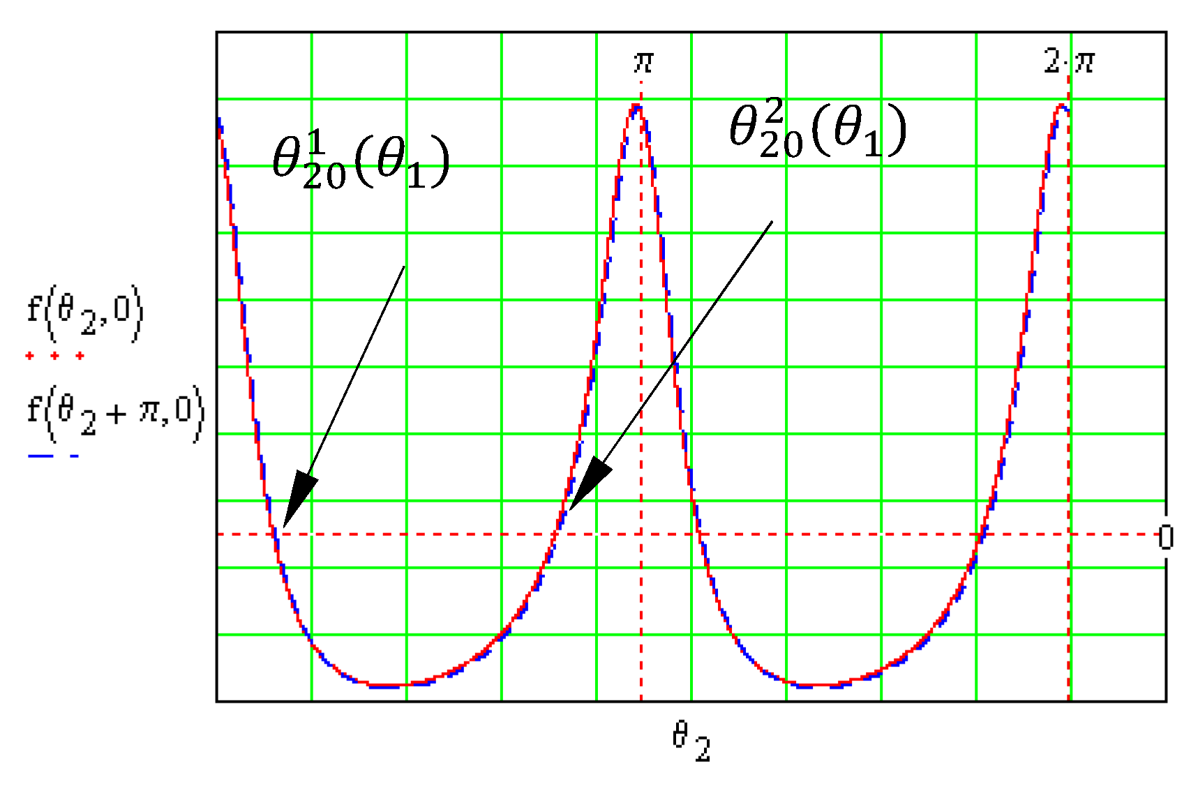
The System (38) has a complicated form, and a numerical procedure was chosen for solving it. In Figure 15, the final angle is represented for a set of constructive parameters () and for a given value of the angle of the driving element . In order to solve the equation using the Newton–Raphson method, the condition that the function must be derivable on an interval in the vicinity of the root must be fulfilled. The equation from the paper is very complex, and it is difficult to test the derivability. Furthermore, if the equation has more than one solution, it is difficult to intuit towards which of these solutions the procedure will converge. For this reason, for solving the equation, the bisection method was chosen [84,85], which requires only the continuity of the function and not the derivability; in addition, the solution of the equation will be found within an interval specified a priori. For a period, two solutions are obtained, and from here, we conclude that the Newton–Raphson method is difficult to apply since the approximate solution for the initialization of the numerical algorithm cannot be specified.
Two main conclusions arise from Figure 15:
- the function , Relation (41), is periodic with respect to variable , with the period ;
- two different solutions of Equation (41) will be found in the closed interval of dimension.
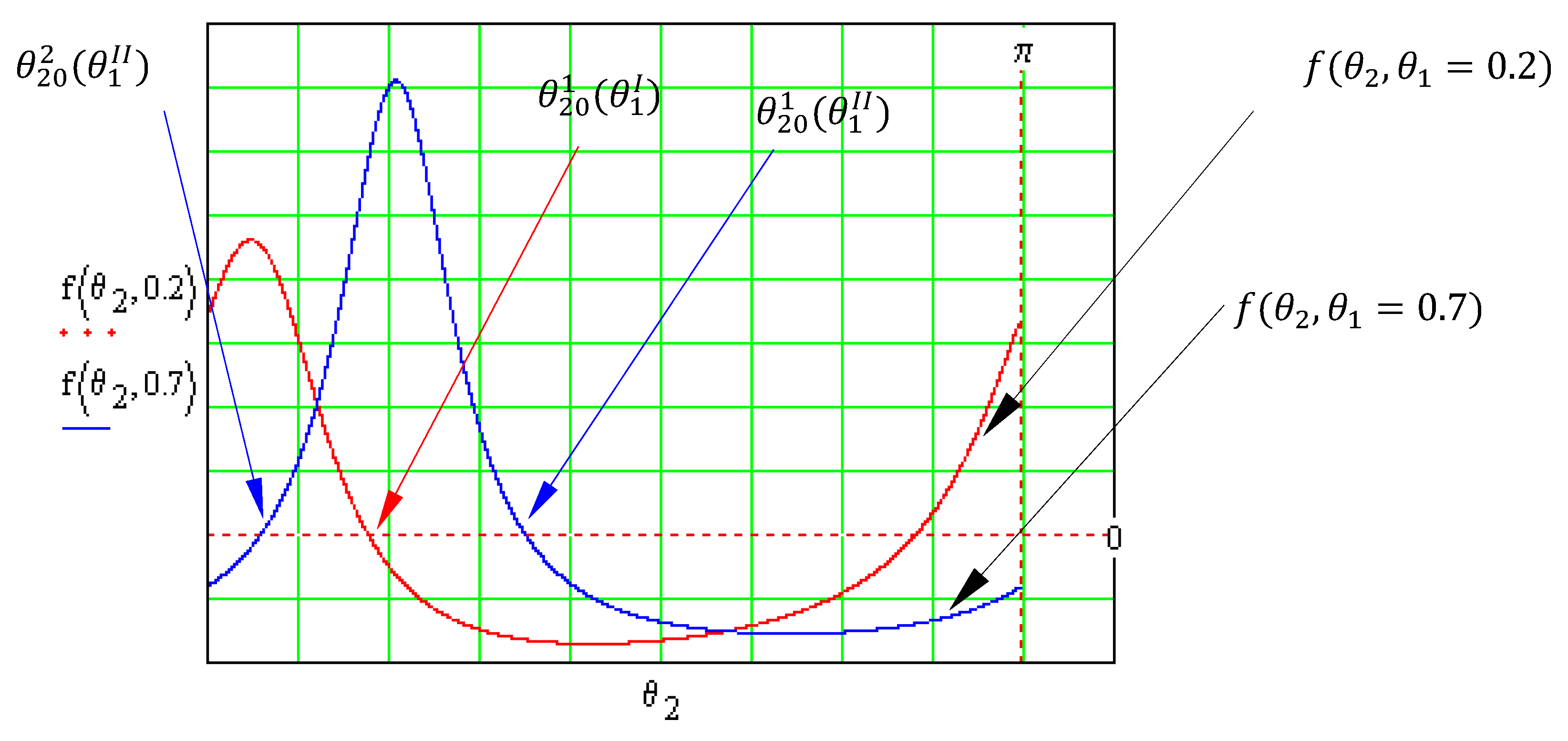
The variations of the function for two positions and of the driving element are represented in Figure 16. The Newton–Raphson algorithm requires the solution of Equation (41). By choosing one of the two solutions for one of assembling alternatives—for instance, (corresponding to the first value of parameter )—when the parameter is changed into , the convergence (which is expected to tend to the solution results in the solution , which corresponds with the second assembling position of the mechanism.
To avoid this situation, the bipartition method was applied while solving Equation (41). The condition imposed on the solving algorithm is that, for the current iteration, the root of the equation should be searched for in an interval with a center identical to the previous iteration root and of length small enough that the two roots will correspond to the same assembling position of the mechanism. The two possible assembling poses of the mechanism are presented in Figure 17.
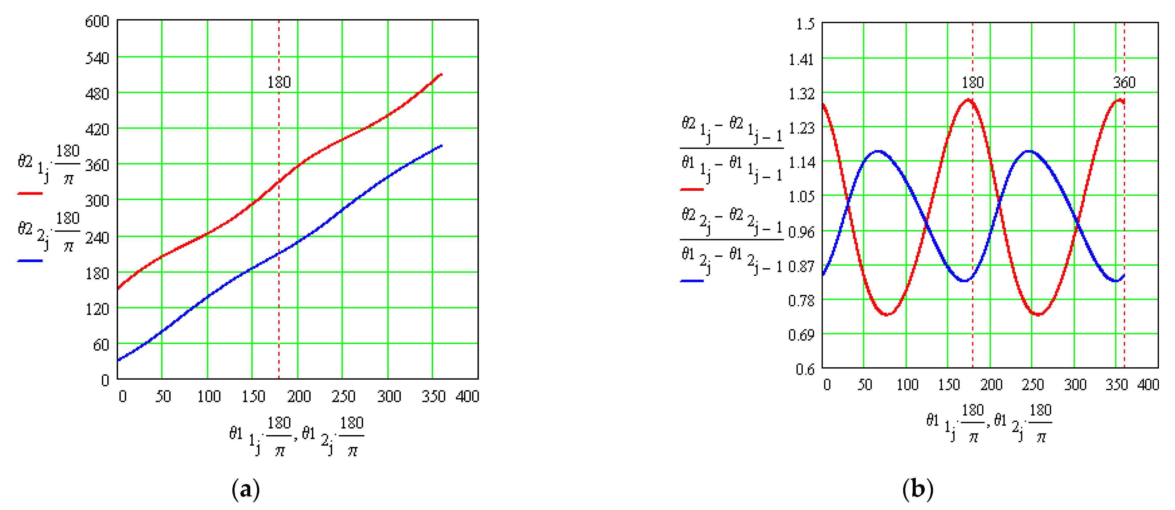
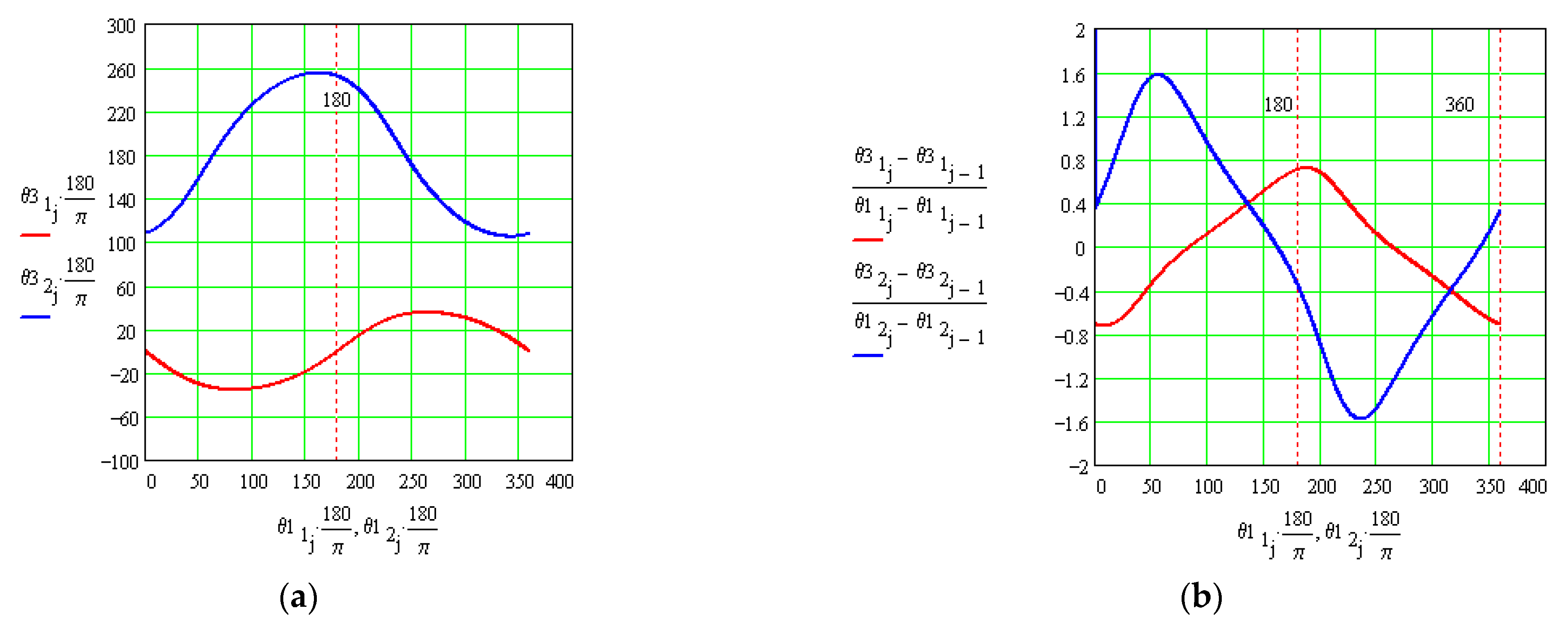
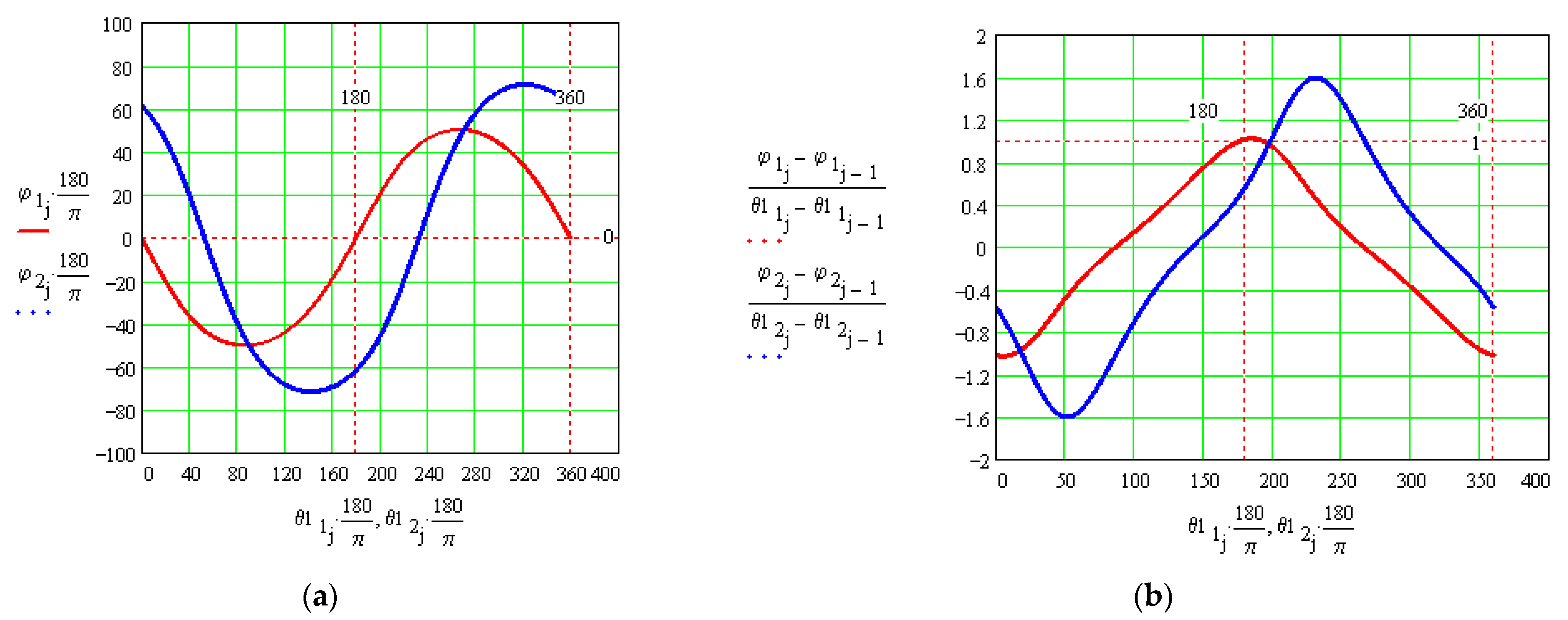
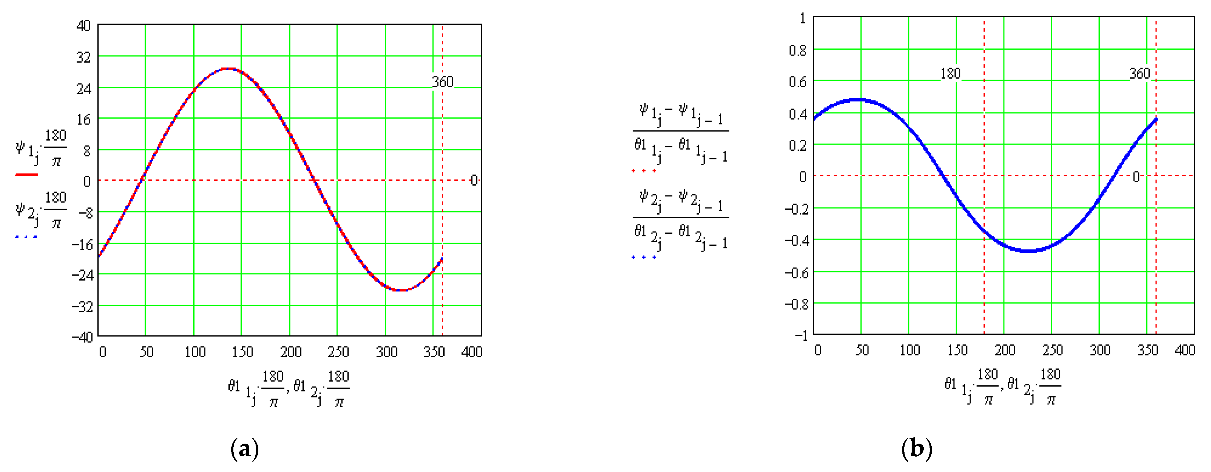
Based on Relation (42), the dependencies and also the angular velocity of the driven element were plotted, as seen in Figure 18. With the known dependency , one can represent , as in Figure 19. Using Relation (44), the trajectory of the center of frame 4 was traced with respect to the driving element, as in Figure 20. The angle of rotation and the angular velocity of the axis of centers in the symmetry plane of the channel were represented by applying Equation (48), as in Figure 21. The basculation angle of the intermediate element around the axis of centers is represented according to Relation (54) in Figure 22.
From Figure 22, one can observe that the oscillations of the intermediate element around the axis of the centers of balls are identical for the two assembling possibilities. This apparent paradox is explained in a simple manner based on Figure 23, in which the angle is the angle between the axis of rotation of the intermediate element and the plane of symmetry of the channel. Denoting with T the intersection point between the axes of rotation of the intermediate element from the two assembling situations, it can be noticed that the oscillation angle is the dihedral angle between the plane of symmetry of the channel, P, and the triangles and . The triangle can be obtained by rotating the triangle around the normal TN, this motion preserves the angle and in consequence .
In order to validate the analytical relations obtained, the kinematics of the mechanism were simulated using dedicated software. The mechanism and the paths of the centers of the balls in the median plane of the channel for the two assembling solutions are presented in Figure 24.
The quantitative validation of the relations obtained in the present work is presented in Figure 25. The paths [86] of the balls’ centers are obtained with the analytical relations, Relations (44), and by kinematical simulation using CATIA software. The Cartesian gridlines enable the quantitative comparison between the two solutions, and a very good agreement is emphasized.
4. Conclusions
The paper presents a new solution for the coupling of two shafts with non-coplanar axes. The proposed structural solution consists of a kinematics chain made of a driving element and a driven element, joined to the ground by revolute pairs of fifth class, and with an intermediate element to connect them. The intermediate part makes to the two shafts a revolute pair and a bipod contact—this consists of two point contacts between a shaft and the middle part. The technical solution for the bipod pair is obtained using two identical metallic spheres assembled together. Both balls are introduced in a parallelepipedal channel of width equal to their diameter. Thus, the presence of the bipod pair will allow for the intermediate element four degrees of freedom with respect to the driving element: three motions for the plane parallel motion of the axis of the centers in the median plane of the channel (two translational and one rotational motion) and a rotational motion of the intermediate part around the axis of the centers of the balls. As a consequence, the bipod contact is a kinematical pair of class two.
The Hartenberg–Denavit homogeneous operators method is applied for the kinematical analysis which requires the replacement of bipod pair to an assembly of cylindrical joints. This solution conducts to complicated calculus because the matrix-loop-closure equation for the equivalent mechanism generates six equations containing both the kinematics parameters of the actual mechanism and the positional parameters of the motions from the fictive joints of the equivalent mechanism. To overcome this difficulty, the geometrical condition of definition of bipod pair is applied. Actually, the bipod pair works when the center of each ball is placed in the median plane of the prismatic channel from the conjugate part. These conditions are expressed in vector form, but the vectors from the equations of condition are known by their projections in different Cartesian systems. Therefore, in order to obtain the equations of projection corresponding to the vector equations, all vectors must be expressed in a unique coordinate system. The Hartenberg–Denavit method is convenient for this requirement since is based on the manner of coordinate transformation of a point when the reference frame is changed.
A problem of utmost importance is the selection of the coordinate system in which the equations of geometrical conditions for the bipod pair should take the simplest form. It is shown that in actuality, using any coordinate system arrives at the same form of scalar equations of condition.
The vector equations of condition are projected and a system of two scalar equation results with unknown position angles from the inner rotational pair and from the exit pair. These equations are linear with respect to the sine and cosine functions of the unknown angles. The direct solving of the system of equations gives expressions of the two unknowns described by inverse trigonometrical functions of one variable, which present the disadvantage that the co-domain has the dimension —a fact that may bring us to solutions that do not correspond to physical reality.
To avoid this aspect, the system of two equations with respect to the sine and cosine of the rotation angle from the driven joint was solved and afterwards, applying the fundamental relations of trigonometry, a trigonometrical equation is obtained, with unknown the rotation angle from the intermediate pair. It was observed that for each value of the rotation angle from the driving pair, the equation has two solutions, fact that attest two different assembling positions of the mechanism for the same position of the driving element.
For a succession of equidistant values of the rotation angle corresponding to a complete rotation of the driven element, the trigonometrical equation obtained was numerically solved, for both assembling solutions, using the bipartition method. The problem of the accuracy of the algorithm used for solving the problem refers to a single transcendental equation and the software allows for a priori stipulation of the accuracy. The advantage of the method consists in the fact that all other kinematical parameters can be expressed analytically as a function of the solution of this equation, and thus the accuracy is controlled. It was noticed that the motion in the intermediate revolute joint is an oscillatory motion with the period half of that of the driving element. With known values of the rotation angle from the intermediate pair, the rotation angle from the exit revolute pair was found using inverse trigonometrical functions of two variables, whose co-domain has the dimension . It was remarked that the rotational motion of the driven element is a rotatory motion with the period equal to the period of the driving element.
Next, the motions from the bipod pair were found. First, the characteristics of the plane parallel motion of the axis of the centers in the median plane of the channel were found for both assembling solutions. More specifically, the motion of the origin of the frame attached to the intermediate element with respect to the frame attached to the driving element was established together with the rotation angle of the axis of centers in the median plane of the prismatic channel. For the last motion—the rotation of the intermediate element around the axis of centers—after the rotation angle was found, it was confirmed that this motion is identical for the two assembling alternatives of the mechanism, a fact perfectly justified but difficult to perceive.
For all rotation motions, the corresponding angular velocities were obtained by numerical division. Of these, of particular helpfulness is the angular velocity of the driven shaft, as it permits the estimation of the transmission ratio of the coupling.
In order to validate the proposed kinematical solution, the trajectory of the center of a ball obtained with the relations deduced in the present paper and the trajectory obtained using a software dedicated to kinematical simulation are presented in comparison; of note is the perfect similarity between the two diagrams.
Author Contributions
Conceptualization, S.A., I.D., F.-C.C., I.-C.R. and I.A.D.; Methodology, S.A., I.D., F.-C.C., I.-C.R. and I.A.D.; Software, S.A., I.D., F.-C.C., I.-C.R. and I.A.D.; Writing—original draft, S.A., I.D., F.-C.C., I.-C.R. and I.A.D. All authors contributed equally to this work. All authors have read and agreed to the published version of the manuscript.
Funding
This research received no external funding.
Institutional Review Board Statement
Not applicable.
Informed Consent Statement
Not applicable.
Data Availability Statement
Not applicable.
Conflicts of Interest
The authors declare no conflict of interest.
References
- Popenda, A.; Szafraniec, A.; Chaban, A. Dynamics of Electromechanical Systems Containing Long Elastic Couplings and Safety of Their Operation. Energies 2021, 14, 7882. [Google Scholar] [CrossRef]
- Birlescu, I.; Husty, M.; Vaida, C.; Gherman, B.; Tucan, P.; Pisla, D. Joint-Space Characterization of a Medical Parallel Robot Based on a Dual Quaternion Representation of SE(3). Mathematics 2020, 8, 1086. [Google Scholar] [CrossRef]
- Kim, S.; Laschi, C.; Trimmer, B. Soft robotics: A bioinspired evolution in robotics. Trends Biotechnol. 2013, 31, 287–294. [Google Scholar] [CrossRef]
- Krivošej, J.; Šika, Z. Optimization and Control of a Planar Three Degrees of Freedom Manipulator with Cable Actuation. Machines 2021, 9, 338. [Google Scholar] [CrossRef]
- Gonçalves, F.; Ribeiro, T.; Ribeiro, A.F.; Lopes, G.; Flores, P. A Recursive Algorithm for the Forward Kinematic Analysis of Robotic Systems Using Euler Angles. Robotics 2022, 11, 15. [Google Scholar] [CrossRef]
- Laski, P.A.; Smykowski, M. Using a Development Platform with an STM32 Processor to Prototype an Inexpensive 4-DoF Delta Parallel Robot. Sensors 2021, 21, 7962. [Google Scholar] [CrossRef]
- Farhadi Machekposhti, D.; Tolou, N.; Herder, J.L. A Review on Compliant Joints and Rigid-Body Constant Velocity Universal Joints Toward the Design of Compliant Homokinetic Couplings. J. Mech. Design 2015, 137, 032301. [Google Scholar] [CrossRef]
- Wittenburg, J. Dynamics of Multibody Systems, 2nd ed.; Springer: Berlin/Heidelberg, Germany, 2008; pp. 9–36. [Google Scholar]
- Lobontiu, N. Compliant Mechanisms: Design of Flexure Hinges; CRC Press LLC: Boca Raton, FL, USA, 2003; pp. 145–206. [Google Scholar]
- Scarfogliero, U.; Stefanini, C.; Dario, P. The use of compliant joints and elastic energy storage in bio-inspired legged robots. Mech. Mach. Theory 2009, 44, 580–590. [Google Scholar] [CrossRef]
- Trease, B.P.; Moon, Y.-M.; Kota, S. Design of Large-Displacement Compliant Joints, J. Mech. Des. 2005, 127, 788–798. [Google Scholar] [CrossRef]
- Midha, A.; Howell, L.L.; Norton, T.W. Limit positions of compliant mechanisms using the pseudo-rigid-body model concept. Mech. Mach. Theory 2000, 35, 99–115. [Google Scholar] [CrossRef]
- Deshmukha, B.; Pardeshib, S.; Roohshad Mistryc, R.; Kandharkard, S.; Waghe, S. Development of a Four bar Compliant Mechanism using Pseudo Rigid Body Model (PRBM). Procedia Mater. Sci. 2014, 6, 1034–1039. [Google Scholar] [CrossRef]
- Marghitu, D.B.; Zhao, J. Impact of a Multiple Pendulum with a Non-Linear Contact Force. Mathematics 2020, 8, 1202. [Google Scholar] [CrossRef]
- Gogu, G. Mobility of mechanisms: A critical review. Mech. Mach. Theory 2005, 40, 1068–1097. [Google Scholar] [CrossRef]
- Müller, A. Generic mobility of rigid body mechanisms. Mech. Mach. Theory 2009, 44, 1240–1255. [Google Scholar] [CrossRef]
- Uicker, J.J., Jr.; Pennock, G.R.; Shigley, J.E. Theory of Mechanisms and Machines, 3rd ed.; Oxford University Press: New York, NY, USA, 2008; pp. 368–400. [Google Scholar]
- Alaci, S.; Ciornei, M.-C.; Filote, C.; Ciornei, F.-C.; Gradinariu, M.-C. Considerations upon applying tripodic coupling in artificial hip joint. IOP Conf. Ser. Mater. Sci. Eng. 2016, 147, 012074. [Google Scholar]
- Urbinati, F.; Pennestrì, E. Kinematic and Dynamic Analyses of the Tripode Joint. Multibody Syst. Dyn. 1998, 2, 355–367. [Google Scholar] [CrossRef]
- Seherr-Thoss, H.C.; Schmelz, F.; Aucktor, E. Universal Joints and Driveshafts. Analysis, Design, Applications, 2nd ed.; Springer: Berlin/Heidelberg, Germany, 2006; pp. 53–79, 109–245. [Google Scholar]
- Watanabe, K.; Kawakastu, T.; Nakao, S. Kinematic and static analyses of tripod constant velocity joints of the spherical end spider type. ASME J. Mech. Des. 2005, 127, 1137–1144. [Google Scholar] [CrossRef]
- Mariot, J.P.; K’nevez, J.-Y. Kinematics of tripode transmissions. A new approach. Multibody Syst. Dyn. 1999, 3, 85–105. [Google Scholar] [CrossRef]
- Wang, X.F.; Chang, D.G.; Wang, J.Z. Kinematic investigation of tripod sliding universal joints based on coordinate transformation. Multibody Syst. Dyn. 2009, 22, 97–113. [Google Scholar] [CrossRef]
- Dudiţă, F. Cuplaje Mobile Homocinetice, Mobile Homokinetic Couplings; Tehnică: Bucharest, Romania, 1974; pp. 209–225. (In Romanian) [Google Scholar]
- Tsai, L.-W. Mechanism Design: Enumeration of Kinematic Structures According to Function, 1st ed.; CRC Press: New York, NY, USA, 2000; pp. 179–191. [Google Scholar]
- Shigley, J.E.; Mischke, C.R. Standard Handbook of Machine Design, 2nd ed.; McGraw Hill: New York, NY, USA, 1996; pp. 18.1–18.4. [Google Scholar]
- Persson Bo, N.J. Sliding Friction: Physical Principles and Applications, 2nd ed.; Springer: Berlin/Heidelberg, Germany, 1998; pp. 89–96. [Google Scholar]
- Stolarski, T.A. Tribology in Machine Design, 2nd ed.; Butterworth-Heinemann Linacre House: Oxford, UK, 2000; pp. 232–246. [Google Scholar]
- Ciornei, F.C.; Alaci, S.; Ciogole, V.I.; Ciornei, M.C. Valuation of coefficient of rolling friction by the inclined plane method. IOP Conf. Ser. Mater. Sci. Eng. 2017, 200, 012006. [Google Scholar] [CrossRef]
- Stolarski, T.A.; Tobe, S. Rolling Contacts, 1st ed.; Professional Engineering Publishing: London, UK; Bury St Edmunds, UK, 2000; pp. 55–73. [Google Scholar]
- Handra-Luca, V.; Stoica, I.A. Introducere in Teoria Mecanismelor, Introduction in Mechanisms Theory; Dacia: Cluj-Napoca, Romania, 1982; Volume 1, pp. 20–44. (In Romanian) [Google Scholar]
- Tutunaru, D. Teoria Mecanismelor si Masinilor. Mecanisme Cu Came, Mechanisms and Machines Theory. Cams Mechanisms; Tehnica: Bucharest, Romania, 1964; pp. 117–152. (In Romanian) [Google Scholar]
- Yang, A.T. Calculus of Screws. In Basic Questions of Design Theory; Spillers, W.R., Ed.; Elsevier: Amsterdam, The Netherlands, 1974; pp. 266–281. [Google Scholar]
- Angeles, J. Spatial Kinematic Chains: Analysis-Synthesis-Optimization; Springer: Berlin/Heidelberg, Germany, 1982; pp. 189–218. [Google Scholar]
- Hartenberg, R.; Denavit, J. Kinematic Synthesis of Linkages, 1st ed.; McGraw-Hill Inc.: New York, NY, USA, 1964; pp. 343–368. [Google Scholar]
- Haslwanter, T. 3D Kinematics; Springer: Cham, Switzerland, 2018; pp. 29–54, 129–133. [Google Scholar]
- Jacob, J.E.; Manjunath, N. Robotics Simplified: An Illustrative Guide to Learn Fundamentals of Robotics, Including Kinematics, Motion Control, and Trajectory Planning; BPB Publications: New Dehli, India, 2022; pp. 228–258. [Google Scholar]
- Jazar, R.N. Theory of Applied Robotics: Kinematics, Dynamics, and Control, 3rd ed.; Springer: Cham, Switzerland, 2022; pp. 225–289. [Google Scholar]
- Gallardo-Alvarado, J.; Gallardo-Razo, J. Mechanisms: Kinematic Analysis and Applications in Robotics (Emerging Methodologies and Applications in Modelling, Identification and Control), 1st ed.; Elsevier: Amsterdam, The Netherlands; Academic Press: London, UK, 2022; pp. 206–211. [Google Scholar]
- Martínez, O.; Campa, R. Comparing Methods Using Homogeneous Transformation Matrices for Kinematics Modeling of Robot Manipulators. In Multibody Mechatronic Systems, Mechanisms and Machine Science, Proceedings of the MuSMe Conference, Córdoba, Argentina, 13–16 October 2020; Pucheta, M., Cardona, A., Preidikman, S., Hecker, R., Pucheta, M., Cardona, A., Preidikman, S., Hecker, R., Eds.; Springer: Cham, Switzerland, 2021; Volume 94. [Google Scholar] [CrossRef]
- Campa, R.; Bernal, J. Analysis of the Different Conventions of Denavit-Hartenberg Parameters. Int. Rev. Model. Simul. (IREMOS) 2019, 12, 45–55. [Google Scholar] [CrossRef]
- Rokbani, N.; Neji, B.; Slim, M.; Mirjalili, S.; Ghandour, R. A Multi-Objective Modified PSO for Inverse Kinematics of a 5-DOF Robotic Arm. Appl. Sci. 2022, 12, 7091. [Google Scholar] [CrossRef]
- Huczala, D.; Kot, T.; Pfurner, M.; Heczko, D.; Oščádal, P.; Mostýn, V. Initial Estimation of Kinematic Structure of a Robotic Manipulator as an Input for Its Synthesis. Appl. Sci. 2021, 11, 3548. [Google Scholar] [CrossRef]
- Klug, C.; Schmalstieg, D.; Gloor, T.; Arth, C. A Complete Workflow for Automatic Forward Kinematics Model Extraction of Robotic Total Stations Using the Denavit-Hartenberg Convention. J. Intell. Robot. Syst. 2018, 95, 311–329. [Google Scholar] [CrossRef]
- Faria, C.; Vilaca, J.L.; Monteiro, S.; Erlhagen, W.; Bicho, E. Automatic Denavit-Hartenberg Parameter Identification for Serial Manipulators. In Proceedings of the IECON Annual Conference of the IEEE Industrial Electronics Society, Lisbon, Portugal, 14–17 October 2019. [Google Scholar]
- Zhang, Y.; Han, H.; Zhang, H.; Xua, Z.; Xiong, Y.; Hana, K.; Li, Y. Acceleration analysis of 6-RR-RP-RR parallel manipulator with offset hinges by means of a hybrid method. Mech. Mach. Theory 2022, 169, 104661. [Google Scholar] [CrossRef]
- Yang, A.T.; Freudenstein, F. Application of Dual-Number Quaternion Algebra to the Analysis of Spatial Mechanisms. J. Appl. Mech. 1964, 31, 300–308. [Google Scholar] [CrossRef]
- Yang, A.T. Displacement analysis of spatial five link mechanisms using (3 × 3) matrices with dual number elements. ASME J. Eng. Indus. 1969, 91, 152–157. [Google Scholar] [CrossRef]
- Roth, B. On the Screw Axes and Other Special Lines Associated With Spatial Displacements of a Rigid Body. J. Eng. Ind. 1967, 89, 102–110. [Google Scholar] [CrossRef]
- Perez, A.; McCarthy, M.; Bennett, B. Dual Quaternion Synthesis of Constrained Robots. In Advances in Robot Kinematics; Springer: Dordrecht, The Netherlands, 2002; pp. 443–452. [Google Scholar]
- Alaci, S.; Buium, F.; Ciornei, F.-C.; Dobincă, D.-I. Tetrapod coupling. Mech. Mach. Sci. 2018, 57, 349–356. [Google Scholar] [CrossRef]
- Ciornei, F.C.; Doroftei, I.; Alaci, S.; Prelipcean, G.; Dulucheanu, C. Analytical kinematics for direct coupled shafts using a point-surface contact. IOP Conf. Ser. Mater. Sci. Eng. 2018, 444, 052002. [Google Scholar] [CrossRef]
- Alaci, S.; Ciornei, F.C.; Filote, C. Considerations upon a new tripod joint solution. Mechanika 2013, 5, 567–574. [Google Scholar] [CrossRef]
- Alaci, S.; Ciornei, F.-C.; Amarandei, D.; Băeşu, M.; Mihăilă, D. On direct coupling of two shafts. Part1: Structural consideration. Tehnomus 2017, 24, 277–280. [Google Scholar]
- Ciornei, F.-C.; Amarandei, D.; Alaci, S.; Romanu, I.-C.; Baesu, M. On direct coupling of two shafts. Part 2: Kinematical analysis. Tehnomus 2017, 24, 281–285. [Google Scholar]
- McCarthy, J.M.; Soh, G.S. Geometric Design of Linkages; Springer: Berlin/Heidelberg, Germany, 2010; pp. 253–279. [Google Scholar]
- McCarthy, J.M. Introduction in Theoretical Kinematics, 3rd ed.; MIT Press: Cambridge, MA, USA, 2018; pp. 103–108. [Google Scholar]
- Alaci, S.; Ciornei, F.C. Elemente de Cinematică Spaţială cu Aplicaţii în Robotică şi Teoria Mecansimelor, Elements of Spatial Kinematics Applied in Robotics and Mechanisms Theory; Matrixrom: Bucharest, Romania, 2020; pp. 22–48. (In Romanian) [Google Scholar]
- Rama Krishna, K.; Sen, D. Second-order total freedom analysis of 3D objects in a single point contact. Mech. Mach. Theory 2019, 140, 10–30. [Google Scholar]
- Rama Krishna, K.; Sen, D. Motion space analysis of objects in multiple point contacts with applications to form-closure and kinematic pairs. Mech. Mach. Theory 2020, 153, 104001. [Google Scholar]
- Rama Krishna, K.; Sen, D. Transitory second-order reciprocal connection for two surfaces in point contact. Mech. Mach. Theory 2015, 86, 73–87. [Google Scholar] [CrossRef]
- Zhou, Y.B.; Buchal, R.O.; Fenton, F.G.; Tan, F.R. Kinematic Analysis of Certain Spatial Mechanisms Containing Higher Pairs. Mech. Mach. Theory 1995, 30, 705–720. [Google Scholar] [CrossRef]
- Fischer, I.S. Dual Number Methods in Kinematics, Static and Dynamics; CRC Press: Boca Raton, FL, USA, 1999; pp. 27–32. [Google Scholar]
- Cheng, C.; Liu, B.; Li, Y.; Liu, Z.; Yang, S.; Wang, Y. Elastodynamic performance of a spatial redundantly actuated parallel mechanism constrained by two point-contact higher kinematic pairs via a model reduction technique. Mech. Mach. Theory 2022, 167, 104570. [Google Scholar] [CrossRef]
- Bai, S.; Angeles, J. A unified input–output analysis of four-bar linkages. Mech. Mach. Theory 2008, 43, 240–251. [Google Scholar] [CrossRef]
- Bil, T. Kinematic analysis of a universal spatial mechanism containing a higher pair based on tori. Mech. Mach. Theory 2011, 46, 412–424. [Google Scholar] [CrossRef]
- Bil, T. Geometry of a mechanism with a higher pair in the form of two elliptical tori. Mech. Mach. Theory 2010, 45, 185–192. [Google Scholar] [CrossRef]
- Gonzalez-Palacios, M.A.; Angeles, J. Cam Synthesis; Springer Science + Business Media: Dordrecht, The Netherlands, 1993; pp. 56–81, 90–99. [Google Scholar]
- Rothbart, H. Cam Design Handbook; McGraw-Hill: New York, NY, USA, 2004; pp. 139–141. [Google Scholar]
- Angeles, J.; López-Cajún, C.S. Optimization of Cam Mechanisms; Springer Science + Business Media: Dordrecht, The Netherlands, 1991; pp. 153–168. [Google Scholar]
- Alaci, S.; Pentiuc, R.D.; Ciornei, F.-C.; Buium, F.; Rusu, O.T. Kinematics analysis of the swash plate mechanism. IOP Conf. Ser. Mater. Sci. Eng. 2019, 568, 012017. [Google Scholar] [CrossRef]
- Akbil, E.; Lee, T.W. On the motion characteristics of tripode joints. Part 1: General case. ASME J. Mech. Transm. Autom. Des. 1984, 106, 228–234. [Google Scholar] [CrossRef]
- Akbil, E.; Lee, T.W. On the motion characteristics of tripode joints. Part 2: Applications. ASME J. Mech. Transm. Autom. Des. 1984, 106, 235–241. [Google Scholar] [CrossRef]
- Akbil, E.; Lee, T.W. Kinematic structure and functional analysis of shaft couplings involving tripode joints. ASME J. Mech. Transm. Autom. Des. 1983, 105, 672–680. [Google Scholar] [CrossRef]
- Lee, T.W.; Akbil, E. General characteristics of the motion of multiple-pode joints. Trans. ASME E J. Appl. Mech. 1984, 51, 171–178. [Google Scholar] [CrossRef]
- K’nevez, J.-Y.; Mariot, J.-P.; Moreau, L.; Diaby, M.P. Kinematics of Transmissions Consisting of an Outboard Ball Joint and an Inboard Generalized Tripod Joint. Proc. Inst. Mech. Eng. K J. Multibody Dyn. 2001, 215, 119–132. [Google Scholar]
- Uicker, J.J.; Denavit, J.; Hartengerg, R.S. An iterative method for the Displacement Analysis of Spatial Mechanisms. J. Appl. Mech. 1964, 31, 309–314. [Google Scholar] [CrossRef]
- Phillips, J. Freedom in Machinery; Cambridge University Press: Cambridge, UK, 2007; pp. 119–120. [Google Scholar]
- Johnson, K.L. Contact Mechanics; Cambridge University Press: Cambridge, UK, 1985; pp. 84–106. [Google Scholar]
- Shtaerman, M. Contact Problems in the Theory of Elasticity; Gostehizdat: Moskow, Russia, 1949; pp. 186–227. (In Russian) [Google Scholar]
- Denavit, J.; Hartenberg, R.S. A Kinematic Notation for Lower-Pair Mechanisms Based on Matrices. J. Appl. Mech. 1955, 22, 215–221. [Google Scholar] [CrossRef]
- Hahn, B.H.; Valentine, D.T. Essential Matlab for Engineers and Scientists, 4th ed.; Academic Press: Oxford, UK, 2009; pp. 92–93. [Google Scholar]
- Maxfield, B. Engineering with Mathcad; Butterworth-Heinemann Elsevier: Oxford, UK, 2006; pp. 287–289. [Google Scholar]
- Dukkipati, R. Numerical Methods, 1st ed.; Anshan Publishers: Tunbridge Wells, UK, 2011; p. 76. [Google Scholar]
- Sauer, T. Numerical Analysis, 2nd ed.; Pearson Education Inc.: Boston, MA, USA, 2012; pp. 25–30. [Google Scholar]
- Ionescu, G.D. Teoria Diferentiala a Curbelor si Suprafetelor, Differential Theory of Curves and Surfaces; Dacia: Cluj-Napoca, Romania, 1984; pp. 53–83. (In Romanian) [Google Scholar]
Figure 1.
Expressing the position of a point M in two different coordinate systems.

Figure 2.
Cylindrical joint between the parts 1 and 2.

Figure 3.
The Hartenberg–Denavit convention.

Figure 4.
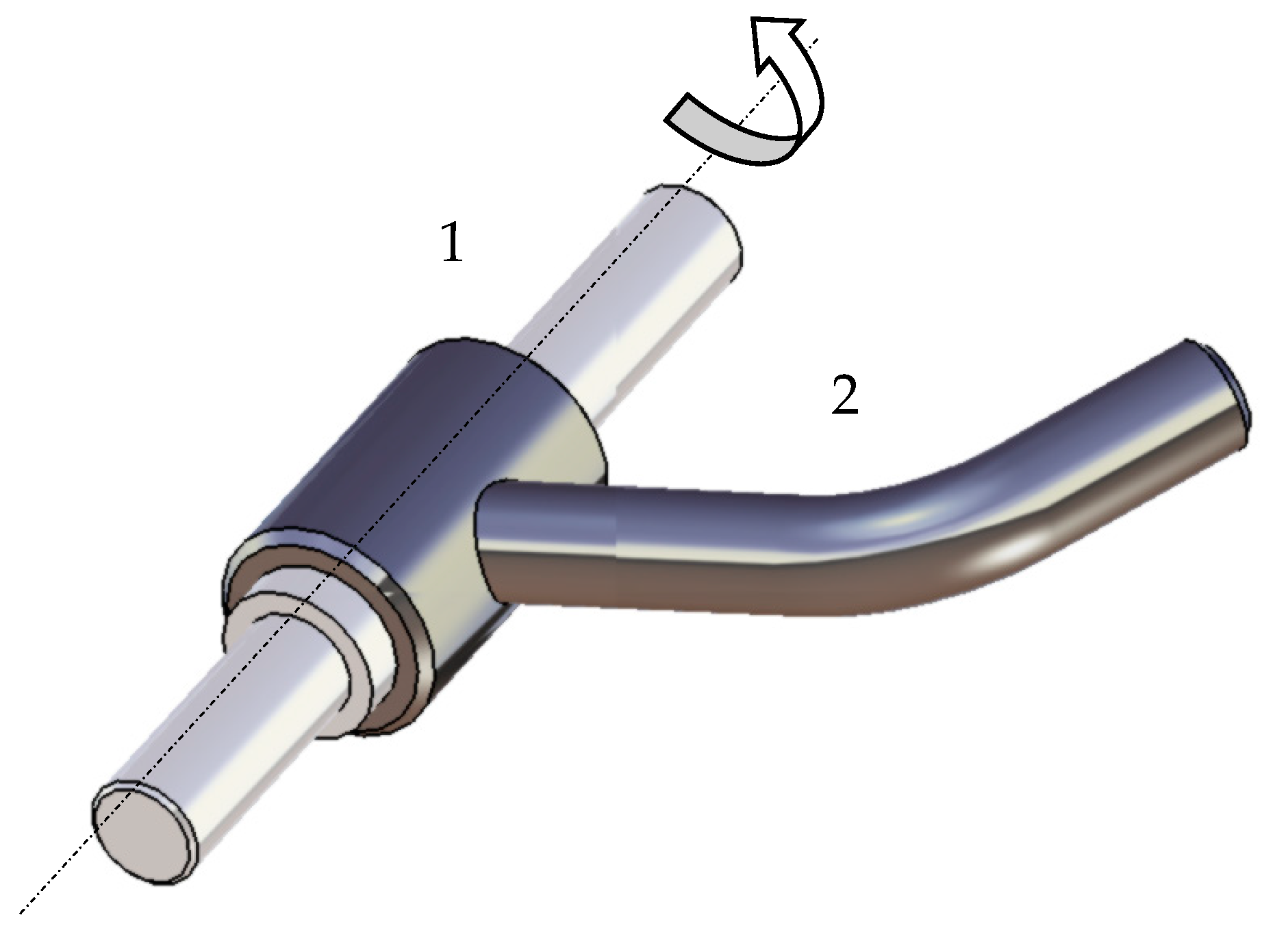
Two shafts (elements 1 and 2) coupled by an intermediate element (3).

Figure 5.
The revolute joint between the elements 1 and 2.

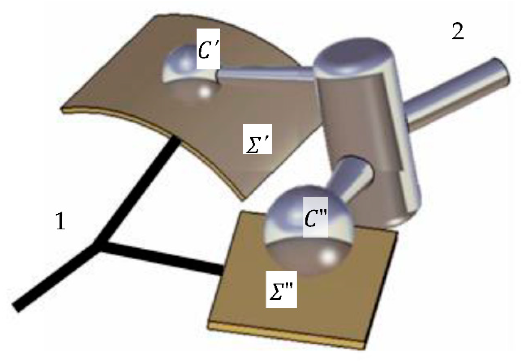
Figure 6.
The bipod joint.

Figure 7.
Technical constructive solutions for bipod joint.

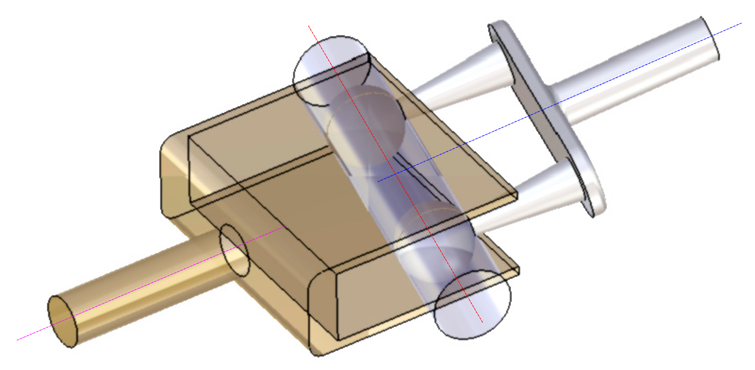
Figure 8.
The bipod contact between the centers of spheres from the element 3 (the intermediate part between the shafts 1 and 2) and the symmetry plane of the channel. The higher pairs are denoted c1 and the revolute pairs are denoted c5.
Figure 8.
The bipod contact between the centers of spheres from the element 3 (the intermediate part between the shafts 1 and 2) and the symmetry plane of the channel. The higher pairs are denoted c1 and the revolute pairs are denoted c5.

Figure 9.
Constructive solution for contact stress reduction in the contact of the bipod pair: (a) direct contact sphere-plane; (b) intermediate pads for stress diminution; (c) assembly of the higher pair.
Figure 9.
Constructive solution for contact stress reduction in the contact of the bipod pair: (a) direct contact sphere-plane; (b) intermediate pads for stress diminution; (c) assembly of the higher pair.

Figure 10.
Constructive solution of the bipod pair.

Figure 11.
Tripod joint, point–surface contact.

Figure 12.
Tripod joint with curve–curve contact.

Figure 13.
Coordinate systems and the constructive and positional parameters of the mechanism.

Figure 14.
Simple displacements from the bipod joint.

Figure 15.
Plot of the rotation angle of the final element for a given constructive configuration and driving angle.
Figure 15.
Plot of the rotation angle of the final element for a given constructive configuration and driving angle.

Figure 16.
The convergence shift in the numerical algorithm.

Figure 17.
The two possible assembling poses of the mechanism.

Figure 18.
The angle of rotation (a) and the angular velocity of the driven element (b).

Figure 19.
The angle of rotation (a) and the angular velocity (b) of the intermediate element with respect to the driven element.
Figure 19.
The angle of rotation (a) and the angular velocity (b) of the intermediate element with respect to the driven element.

Figure 20.
The path of the origins of the frame attached to the intermediate element in the median plane of the channel, for the two assembling possibilities.
Figure 20.
The path of the origins of the frame attached to the intermediate element in the median plane of the channel, for the two assembling possibilities.

Figure 21.
The angle of rotation (a) and the angular velocity of the axis of centers in the middle plane of the channel (b).
Figure 21.
The angle of rotation (a) and the angular velocity of the axis of centers in the middle plane of the channel (b).

Figure 22.
The angle of basculation (a) and the corresponding angular velocity (b) of the intermediate element with respect to the axis of centers.
Figure 22.
The angle of basculation (a) and the corresponding angular velocity (b) of the intermediate element with respect to the axis of centers.

Figure 23.
Identical oscillation angles of the intermediate element for the two assembling cases.

Figure 24.
Kinematics simulation of the paths of the centers of the balls in the median plane of the channel for the two assembling solutions.
Figure 24.
Kinematics simulation of the paths of the centers of the balls in the median plane of the channel for the two assembling solutions.

Figure 25.
Quantitative assessment of the tracks of the balls’ centers in the symmetry plane of the channel: (a) present analytical relations plotted in Mathcad; (b) kinematics simulation in CATIA.
Figure 25.
Quantitative assessment of the tracks of the balls’ centers in the symmetry plane of the channel: (a) present analytical relations plotted in Mathcad; (b) kinematics simulation in CATIA.

Publisher’s Note: MDPI stays neutral with regard to jurisdictional claims in published maps and institutional affiliations. |
© 2022 by the authors. Licensee MDPI, Basel, Switzerland. This article is an open access article distributed under the terms and conditions of the Creative Commons Attribution (CC BY) license (https://creativecommons.org/licenses/by/4.0/).
Share and Cite
MDPI and ACS Style
Alaci, S.; Doroftei, I.; Ciornei, F.-C.; Romanu, I.-C.; Doroftei, I.A. The Kinematics of a Bipod R2RR Coupling between Two Non-Coplanar Shafts. Mathematics 2022, 10, 2898. https://doi.org/10.3390/math10162898
AMA Style
Alaci S, Doroftei I, Ciornei F-C, Romanu I-C, Doroftei IA. The Kinematics of a Bipod R2RR Coupling between Two Non-Coplanar Shafts. Mathematics. 2022; 10(16):2898. https://doi.org/10.3390/math10162898
Chicago/Turabian StyleAlaci, Stelian, Ioan Doroftei, Florina-Carmen Ciornei, Ionut-Cristian Romanu, and Ioan Alexandru Doroftei. 2022. "The Kinematics of a Bipod R2RR Coupling between Two Non-Coplanar Shafts" Mathematics 10, no. 16: 2898. https://doi.org/10.3390/math10162898
Note that from the first issue of 2016, this journal uses article numbers instead of page numbers. See further details here.