Article

Cloudformer V2: Set Prior Prediction and Binary Mask Weighted Network for Cloud Detection

1
School of Information Science and Technology, North China University of Technology, Beijing 100144, China
2
College of Information Science and Technology, Beijing University of Chemical Technology, Beijing 100029, China
*
Author to whom correspondence should be addressed.
Mathematics 2022, 10(15), 2710; https://doi.org/10.3390/math10152710
Submission received: 30 June 2022 / Revised: 28 July 2022 / Accepted: 29 July 2022 / Published: 31 July 2022

Abstract

:
Cloud detection is an essential step in optical remote sensing data processing. With the development of deep learning technology, cloud detection methods have made remarkable progress. Among them, researchers have started to try to introduce Transformer into cloud detection tasks due to its excellent performance in image semantic segmentation tasks. However, the current Transformer-based methods suffer from training difficulty and low detection accuracy of small clouds. To solve these problems, this paper proposes Cloudformer V2 based on the previously proposed Cloudformer. For the training difficulty, Cloudformer V2 uses Set Attention Block to extract intermediate features as Set Prior Prediction to participate in supervision, which enables the model to converge faster. For the detection of small clouds, Cloudformer V2 decodes the features by a multi-scale Transformer decoder, which uses multi-resolution features to improve the modeling accuracy. In addition, a binary mask weighted loss function (BW Loss) is designed to construct weights by counting pixels classified as clouds; thus, guiding the network to focus on features of small clouds and improving the overall detection accuracy. Cloudformer V2 is experimented on the dataset from GF-1 satellite and has excellent performance.

1. Introduction

With the development of remote sensing technology, the requirements for processing remote sensing data have increased, and researchers have therefore proposed a variety of efficient and accurate processing methods [1,2]. The quality of optical remote sensing images has been significantly improved. Sub-meter remote sensing data is becoming more and more common, and applications are expanding. However, optical remote sensing is highly susceptible to weather factors, one of which is cloud cover, which forms highly reflective regions in the acquired images. When the image contains many clouds, its application value will be greatly reduced [3]. Automated cloud detection methods can help researchers evaluate and process optical remote sensing data and improve the efficiency of remote sensing data analysis. Therefore, numerous scholars focus on the research of high-precision cloud detection methods.
Over the years, many cloud detection methods have emerged [4]. In the early days, cloud detection methods were dominated by traditional image processing methods [5,6,7]. Starting from 2016, with the development of deep learning technology, cloud detection methods based on deep learning have gradually occupied the mainstream [8,9,10,11,12], and they are characterized by high automation, high accuracy, and high generalizability. The cloud detection task can basically be regarded as a dichotomous image semantic segmentation task, so the development of image semantic segmentation algorithms also drives the progress of cloud detection technology. Advanced results have been achieved in cloud detection methods based on convolutional neural networks. For example, GCDB-UNet [13] and DABNet [14] are based on a fully convolutional neural network. However, the current methods based on the full convolutional neural network architecture have shown bottlenecks and it is difficult to further improve the detection accuracy.
With the advancement of semantic segmentation methods, Transformer-based network architecture is introduced to computer vision tasks [15,16], which shows excellent performance with the powerful feature modeling capability of the multi-headed attention mechanism. Transformer network segments images into multiple non-overlapping patches, and transforms these patches into tokens, which are fed into the multi-headed attention mechanism. The attention mechanism establishes connections among the different patches for feature extraction.
Although the Transformer has excellent modelling capabilities, it ignores the connection relationships between elements within patches, resulting in reduced detection accuracy when the target size is small [17]. In addition, the Transformer’s global self-attention calculation is also detrimental to the image processing task [18]. In contrast with language, which has high semantic and information density, images, as natural signals, have severe information redundancy. Language has a stronger need for global understanding, while image information is more concerned with the connections between adjacent features [19]. At the same time, the overly free computation, which is devastatingly disastrous for training, makes it difficult to converge for the Transformer. Cloudformer [20] has tried to introduce the Transformer model to cloud detection tasks with excellent results. However, due to the problems mentioned above, Cloudformer still has several drawbacks: (1) long training rounds, large amount of data required for training, and difficulty in convergence. (2) the detection rate of small clouds is strongly influenced by the imbalance between positive and negative samples.
To address these problems, we propose Cloudformer V2, which is based on Cloudformer [20]. The problem of slow training and difficult convergence is addressed by using an a priori ensemble prediction branch to extract intermediate features to assist the supervised network. The multi-scale Transformer decoder will model features at multiple scales, while the binary mask-weighted loss function (BW Loss) increases the weight of small cloud data during training, and they enhance the network’s small cloud detection capability.
The rest of the paper is organized as follows. In Section 2, we describe our approach in detail. Section 3 shows the experimental results. Section 4 discusses the overall design details and analyses the experimental results. Finally, Section 5 concludes the overall work.

2. Materials and Methods

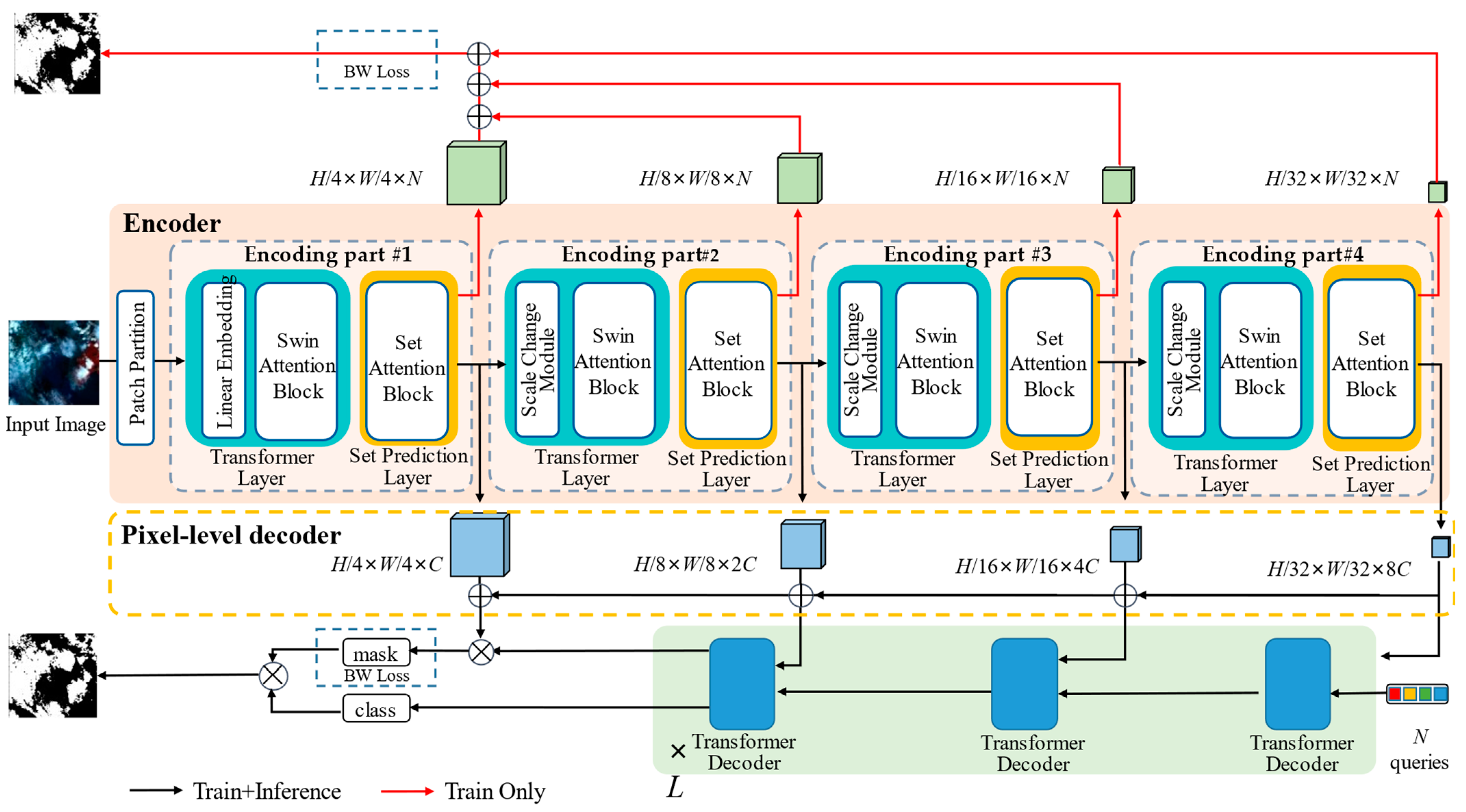
2.1. Overall Structure of Cloudformer V2
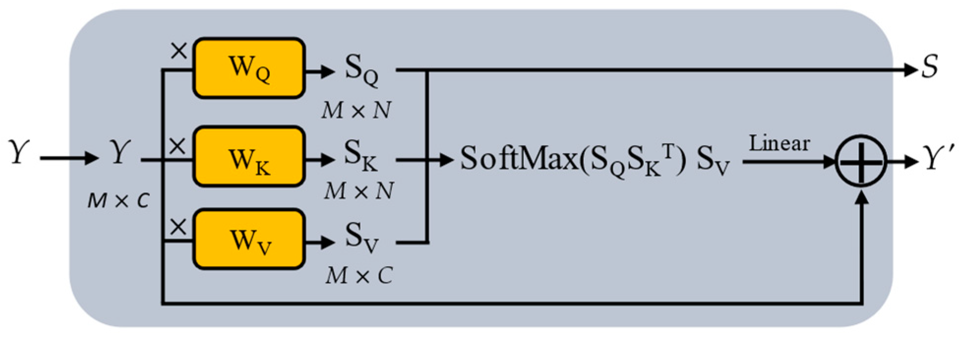
The overall structure of the proposed Cloudformer V2 is shown in Figure 1. The input is first partitioned into non-overlapping patches of 4 × 4 pixels, as smaller patches can be better used for the detection of small-sized clouds. These patches act as tokens to be passed into the encoding part.
The encoding part models the features at four different scales, i.e., 1/4, 1/8, 1/16 and 1/32 of the original image resolution. Each encoding part consists of two layers: (1) Transformer layer, which is a stack of the Scale Change module and the Swin Transformer module: (2) Set Prediction layer, which consists of Set Attention Block and is responsible for extracting intermediate Set Prior Predictions. The Set Prediction layer uses the features of the Transformer layer to encode and return an intermediate Set Prior mapping.
As shown by the red line in Figure 1, a lightweight upsampling decoder is used to aggregate the four scales of the Set Prior mapping in order to obtain the Set Prior mask prediction and to supervise it using binary mask weighted loss function (BW Loss) to assist in the training of the whole network. In addition, the Set Prediction layer also gives mask features, which are fed into the Transformer hierarchical decoder in order from lowest to highest resolution, using Feature-aligned Pyramid Network (FaPN) [21] as a pixel-level decoder for resolution reconstruction.
A classification prediction and an ensemble mask prediction are then generated, and their combination is the final output at prediction time. At training time, the final output, together with the a priori ensemble mask prediction, oversees the training of the entire network.

2.2. Encoder

The encoder consists of four encoding parts. Each encoding part consists of two layers: Transformer layer [22] and Set Prediction layer.
The first Transformer layer contains a Linear Embedding layer and a standard Swin Transformer module. The Linear Embedding layer is used to change the feature dimension of the patches. The other Transformer layer contains a Scale Change module and a standard Swin Transformer module, which extracts features from the image. In the Scale Change module, we discard Patch Merging in the last three parts and use a convolution operation to reduce the resolution. The image information is not extremely dependent on long-distance information, so the excessive degrees of freedom of the Transformer are somewhat negative for extracting image features, while convolution is an operation with a strong inductive bias [23], which will impose some limitations on the overall network and thus improve the performance of the Transformer model in image processing tasks. The structure of the Swin Transformer layer not only has good feature extraction capability but also has only linear computational complexity with respect to the image resolution. Each Swin Transformer block is divided into multiple non-overlapping windows, with attention computed only within the windows [24]. Window shifts are used to deal with intersection regions, allowing for efficient image feature modeling.
The Set Prediction layer takes the features extracted by the Transformer layer as input and maps the features to the set space using Set Attention Block with the aim of generating set mask predictions. Set mask prediction is an intermediate feature. By fusing these intermediate features with a pyramid structure and restoring them to the resolution of the original image, a preliminary prediction can be obtained. This prediction is not very accurate. However, they contain the intermediate features of the loss of the final prediction results, so using it to guide the update of weights in the network will help the network converge faster and more stably. In addition, the Set Prior Prediction process only occurs in the training stage. Therefore, such a strategy will not affect the reasoning speed of the final network. Set Attention Block is computed with a single-headed set attention. As shown in Figure 2, Set Attention Block to divide the input features Y into three individuals using the parametrically learnable linear layers WQ, WK and WV: the set query SQ, the set key SK and the feature values SV. The dimension of SV is M × C, where M is the length of the sequence in each window, C is the number of windows. The dimensions of SQ and SK are M × N, respectively, where N is equal to the number of queries set in the Transformer decoder. In this article N is set to 100 as in Cloudformer. SQ returns a priori set predictions, and SQ and SK act together to update SV to acquire Y’ to pass to the next stage. Set attention process is as follows:
S Q = Y · W Q
S K = Y · W K
S V = Y · W V
S e t   A t t e n t i o n ( S Q , S K , S V ) = SoftMax ( S Q S K T ) S V
Y = l i n e a r ( S e t   A t t e n t i o n ( S Q , S K , S V ) ) + Y

2.3. Decoder

In the pixel-level decoder, we use FaPN [21] to produce context-aligned multi-scale feature maps. In the Transformer decoder, we provide one resolution feature at a time to one Transformer decoder layer to build a multi-scale Transformer decoding structure [25]. Specifically, multiple resolution features are generated in the pixel-level decoder, and their resolutions are 1/32, 1/16, 1/8 and 1/4 of the original image, respectively. The result of the Transformer decoder is resized through a multilayer perceptron (MLP) layer. Features with 1/4 resolution are embedded and the mask prediction output is obtained by simple upsampling and has dimensions H × W × N. The Transformer decoder is connected to another MLP layer to obtain the classification prediction, which has dimensions K × N. Finally, the mask prediction output and the classification prediction output are combined as the final output of the framework.

2.4. Binary Mask Weighted Loss Function

The detection of small clouds in optical remote sensing images has always been a challenge. When the number of positive samples in the data is too small, it usually leads to the problem of positive and negative sample imbalance. For cloud detection tasks, small clouds contain relatively few pixels, and the presence of a large number of sparse small clouds in an image can lead to the problem of positive and negative sample imbalance. Moreover, the pixel information of small clouds is more likely to be influenced by the surrounding pixels, which leads to the reduction of detection accuracy.
We adopt a masked classification design in the network structure, which has been shown to work well in Cloudformer for cloud detection tasks. Based on the mask classification, we solve the small cloud detection problem by adding weights to the loss function. When the number of cloud pixels contained in the image will be small, the loss will be scaled up as a way to increase the penalty to the network for errors in detecting small clouds. In order to train the masked classification model, we process the labels of the dataset [26] and transform the ground truth N gt into a set z g t = { ( c i g t , m i g t ) |   c i g t { 1 , , K } ,   m i g t { 0 , 1 } H × W } i = 0 N g t . We fill the “no object “ element so that Ngt = N. It can match the output of the framework, where c i g t is the class label corresponding to the i element of the set. m i g t is the binary masks corresponding to the i element of the set. On this basis, a Binary mask Weighted loss function (BW Loss) based on mask classification is proposed to optimize small cloud detection rate fluctuations in the network due to sample imbalance. It is defined as follows:
L B W = j = 1 N [ ω j I g ( c j g t ) ( λ c e L c e + λ d i c e L d i c e ) ]
I g ( c j g t ) = { 1 c j g t = 0 c j g t =
where Lce is the cross-entropy loss and Ldice is the dice loss [27]. As with Mask2former [25], we set λce = 5.0 and λdice = 5.0.
Taking advantage of the mask classification, we calculate the total number of pixels in each set that is classified as a cloud. Loss weights are then calculated for each collection based on the total number of pixels, thereby amplifying the weights of the cloud collections with fewer pixels. Making the network more focused on small cloud pixel sets. Specifically, in Cloudformer V2, the mask set branch gives a set of predictions . belongs to N × H × W and N is the number of queries in Transformer decoder. is the set of N predictions containing cloud features, and we count the number of pixels classified as clouds for each prediction, from which we calculate the weight ωj of the mask loss value for each outcome (a combination of cross-entropy loss and dice loss are used as our mask loss) The procedure for calculating the weights can be expressed as:
ω j = l i n e ( Sigmoid ( h = 0 H w = 0 W p h , w H × W 0.5 ) )
where p is the pixel value in the binary mask prediction, and ωj is mapped to (1,2) by a linear transformation after activation using the Sigmoid function. The Binary mask Weighted loss function is used in the mask classification branch as well as in the ensemble prior prediction branch as an aid to training. In the experimental section, the Binary mask Weighted loss function will be analyzed in detail.

3. Results

3.1. Evaluation Criteria and Data Processing

To evaluate and compare the performances of different methods, three metrics, including Mean Intersection with Union (MIoU) [28], Mean Accuracy (MAcc) [29] and Pixel Accuracy (PAcc) [30] are used. For all experimental data, they can be divided into four cases as follows: true positive (TP), false positive (FP), true negative (TN) and false negative (FN). The resulting metric formula for the evaluation indicator is expressed as follows:
MIoU = 1 k + 1 i = 0 k TP FN + FP + TP
MAcc = 1 k + 1 i = 0 k TP FP + TP
PAcc = TP + TN TP + TN + FP + TN

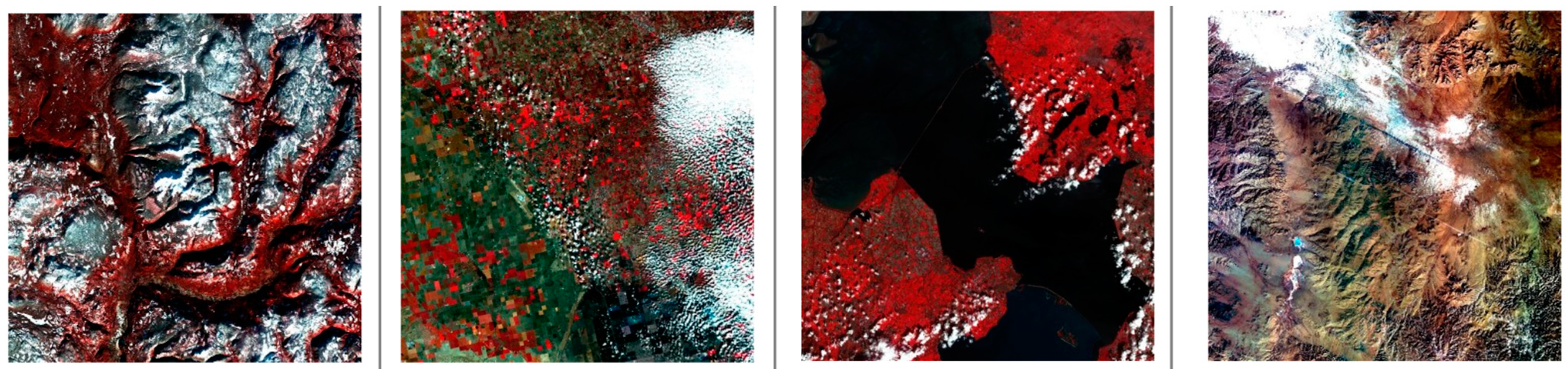
3.2. Cloud Detection Dataset

The experiment data are multispectral data from the GF-1 satellite [31], containing three bands of visible RGB and near-infrared, with a variety of scenes of snowy mountains, cities, water, vegetation, etc. An example is shown in Figure 3.
The data were acquired between May 2021 and December 2021. To construct the dataset for the experiment, we discarded the NIR band and used only the visible band. The data are converted to RGB full color images, which were then enhanced by random cropping and rotation. The dataset contains 10,250 images of 512 × 512 pixel size, divided into training set and test set in the ratio of 8:2, with 8200 images in the training set and 2050 images in the test set.

3.3. Comparisonl Models and Experimental Settings

To illustrate the effectiveness of Cloudformer V2, we compare it with typical cloud detection models and superior semantic segmentation models on the cloud detection dataset. Two cloud detection models, Cloudformer [20] and GCDB-UNet [13] are selected. Moreover, the well-known SwinTransformer-UperNet [32] and Mask2former [25] models for semantic segmentation are also chosen. Cloudformer and GCDB-UNet are recently proposed methods for cloud detection, and they perform well in cloud detection tasks. Swin Transformer includes a sliding window operation and a hierarchical design structure. It has performed well in several tasks in computer vision. Mask2Former is an excellent transformer-base segmentation architecture that has achieved state-of-the-art on several publicly available datasets.
In the experiments, each model is trained on the same dataset with the same dataset partitioning strategy to ensure the comparability of the experiments. In addition, we only detect clouds and do not detect cloud shadows. In the training phase, the batch size is set to 8 and the learning rate warm up radio is set to 10−6. After 1500 iterations, the initial value of 6 × 10⁻⁵ is restored, and the learning rate decays approximately exponentially in the later training. A total of 160,000 iterations are trained. Adam [33] is used as the optimization strategy. The experiments are implemented with the help of MMSegmentation on an NVIDIA RTX2080TI GPU.

3.4. Ablation Experiment

In this subsection, we show ablation experiments on the priori Set Prediction, Set Attention Block, the multi-scale Transformer decoder and the Binary mask Weighted loss function. These experiments form a key basis for analyzing the performance of the Cloudformer V2 model.

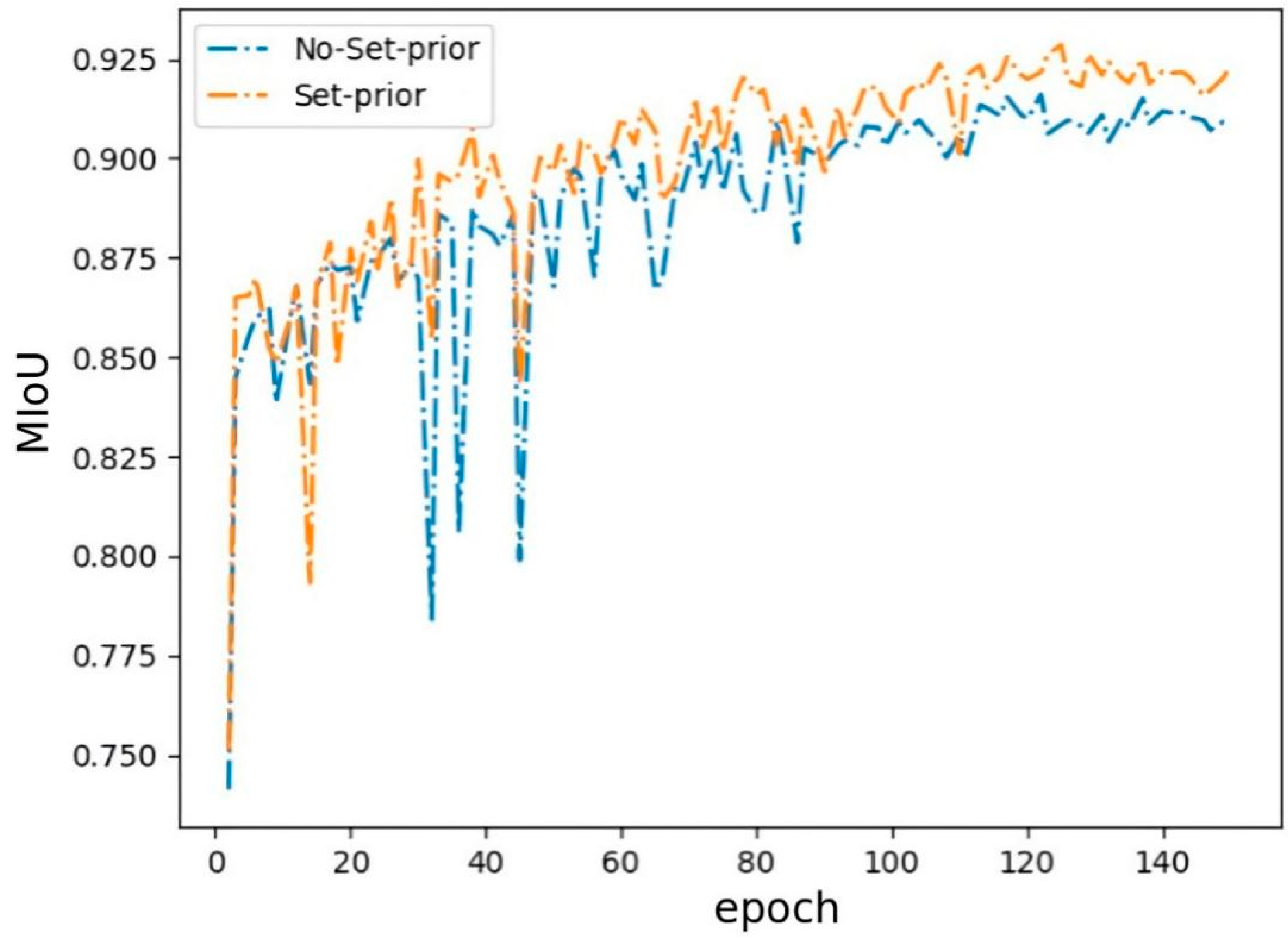
3.4.1. Effect of Set Prior Prediction

The training is carried out in two ways while keeping the rest of the structure the same. One way is to keep the structure in Figure 1 and train it. The other way is to discard the red arrowed part in Figure 1 and no longer separate the Set Prior Predictions from the Set Prediction layer to aid training. In Figure 4, the trend of MIoU for the two training ways is shown. It is clear that Set Prior Prediction improves training efficiency.

3.4.2. Effect of Set Attention Block

To investigate the effect of Set Attention Block on the overall performance, we replace the Set Attention with a normal Attention and block the Set Prior Prediction branch, and the experimental results are shown in Table 1. Set Attention Block can help the framework to improve the prediction accuracy by a small amount.

3.4.3. Effect of Multi-Scale Transformer Decoder

Figure 5a shows the multi-scale transformer decoder structure of the Cloudformer V2 framework, while Figure 5b shows the normal transformer decoder structure. The main difference is that the traditional Transformer decoder only models features at the smallest resolution, which results in a loss of features. The Multi-Scale Transformer decoder, on the other hand, takes in multiple scales of feature maps for modelling, which significantly improves the modelling capability of the network. We compare the overall effect of the two structures on the framework.
Table 2 shows the ablation experiment results and it can be seen that the multi-scale Transformer decoder has performance improvement on the framework. This indicates that the multi-scale transformer decoder is able to make better use of the information in the feature map.

3.4.4. Effect of Binary Mask Weighted Loss Function

To solve the sample imbalance problem of small clouds, the Binary mask Weighted loss function (BW Loss) is proposed in this paper. To verify the contribution of the loss function on the framework, we train the model using two loss functions, i.e., BW Loss and a linear combination of cross-entropy loss and dice loss. The experimental results are shown in Table 3. We quantify its performance by metrics such as MIoU and qualitatively demonstrate the compared results in Figure 6.

3.5. Comparison with State-of-the-Art Methods

Table 4 and Figure 7 show the performance of the Cloudformer V2 framework compared to other methods on GF-1 satellite data. The overall evaluation results show that Cloudformer V2 has a 1 to 3% improvement in accuracy compared to all other recent methods.

4. Discussion

4.1. The Effectiveness of the Transformer Network and Set Attention Block

In terms of receptive field, the Transformer network has a larger receptive field initially compared to the convolutional neural network, which can help the network to obtain more valid information early on [34]. In terms of the core computational mechanism, the convolutional neural network is channel-driven, while the multi-headed attention mechanism is data-driven. The Transformer network can retain more spatial location information, which is very important in cloud detection tasks, so the above advantages make it an excellent feature extractor.
However, the free-form nature of the multi-headed attention mechanism makes it difficult to train the network for convergence, and although in the encoding part we use the Swin Transformer local attention mechanism designed to enhance inductive bias, training is still very difficult. Therefore, we use ensemble prior prediction as an intermediate feature to assist in the training of the entire network. The ensemble prior prediction is obtained by combining a simple single-headed ensemble attention mechanism with bilinear difference upsampling.

4.2. Binary Mask Weighted Loss Function Design and Analysis

When processing remote sensing images, we find that many clouds can be seen in the original image. However, after data enhancement operations such as random cropping, a large number of images in the dataset contain only a few clouds, which leads to positive and negative sample imbalance. The Binary mask Weighted loss function is therefore proposed. Using the binary mask predictions obtained by the multi-scale Transformer as a base, a weight is computed to control the size of the current predicted loss. The smaller the cloud, the greater the weighting, which increases the loss in small cloud scenes and enables the network to learn small cloud scenes more actively, thus reducing the impact of sample imbalance on the network.

4.3. Analysis of Experimental Results

To illustrate the effectiveness of Cloudformer V2, several experiments are designed and performed. In the ablation experiment, Figure 4 shows the performance of set-prior maps. It can be seen that with the set-prior maps structure, the network is able to start converging at an earlier epoch and obtain better results with fewer rounds. The experimental results also show that there is a small reduction in the degree of oscillation during the training process, especially at the 30–50 epoch in the figure. Table 1 then demonstrates the performance gains from Set Attention Block. Table 2 shows that the multi-scale Transformer decoder improves the overall performance of the network, and that the multi-scale structure allows for better use of image information to obtain more accurate predictions. Table 3 shows quantitatively the performance improvement of the Binary mask weighted loss function in GF-1 data. The visualization in Figure 6 further illustrates that the Binary mask Weighted loss function achieves the objectives of our design. From a full graph perspective, the results on the right side ignore the large number of small clouds. The results of the BW loss used on the left side detect the small clouds very well.
Cloudformer V2 performs well in comparison to other advanced methods. In Figure 7, we can visually see that Cloudformer V2 has an advantage in the detection accuracy on small clouds, thin clouds and cloud edges. Table 4 shows that Cloudformer V2 achieves a 1 to 3% improvement in overall accuracy over all other methods.

5. Conclusions

The Cloudformer V2, a high-precision cloud detection method based on Cloudformer is presented in this paper. It focuses on optimizing the Transformer network for slow training in cloud detection tasks and sample imbalance in small cloud scenes. We propose to use ensemble prior prediction-assisted training to optimize the training speed of the network. We also proposed to use the Binary mask Weighted loss function to solve the sample imbalance problem in small cloud detection. The multi-scale Transformer decoder makes more effective use of image information and further improves the overall accuracy. Several experimental results show that Cloudformer V2 outperforms other existing cloud detection methods. In the future, we will be committed to the lightweight work of Cloudformer V2. We hope to find the parts of the framework that have less impact on the final results and improve or delete them. We try to further compress the scale of the model without reducing the accuracy of the framework, so that it can be used for real-time cloud detection tasks on airborne platforms whose performance is lower than that of ground servers. At the same time, we will try to put Cloudformer V2 into other tasks (such as water detection) to further verify the versatility of our method.

Author Contributions

Conceptualization, Z.Z., Z.X. and Q.T.; methodology, Z.Z. and Z.X.; software, Z.X.; validation, Q.T. and Z.X.; formal analysis, Z.X. and C.L.; investigation, Z.Z.; resources, Z.Z. and Z.X.; data curation, Z.Z. and Z.X.; visualization, Z.X.; writing-original draft preparation, Z.X.; writing-review and editing, Z.Z. and Y.Z.; supervision, Y.Z.; project administration, Y.Z. All authors have read and agreed to the published version of the manuscript.

Funding

This research is funded by North China University of Technology Research Start-up Funds.

Conflicts of Interest

The authors declare no conflict of interest.

References

  1. Ma, F.; Zhang, F.; Xiang, D.; Yin, Q.; Zhou, Y. Fast Task-Specific Region Merging for SAR Image Segmentation. IEEE Trans. Geosci. Remote Sens. 2022, 60, 1–16. [Google Scholar] [CrossRef]
  2. Ma, F.; Zhang, F.; Yin, Q.; Xiang, D.; Zhou, Y. Fast SAR Image Segmentation With Deep Task-Specific Superpixel Sampling and Soft Graph Convolution. IEEE Trans. Geosci. Remote Sens. 2022, 60, 1–16. [Google Scholar] [CrossRef]
  3. Hagolle, O.; Huc, M.; Pascual, D.V.; Dedieu, G. A Multi-Temporal Method for Cloud Detection, Applied to FORMOSAT-2, VENS, LANDSAT and SENTINEL-2 Images. Remote Sens. Environ. 2010, 114, 1747–1755. [Google Scholar] [CrossRef] [Green Version]
  4. Mahajan, S.; Fataniya, B. Cloud Detection Methodologies: Variants and Development—A Review. Complex Intell. Syst. 2020, 6, 251–261. [Google Scholar] [CrossRef] [Green Version]
  5. Qiu, S.; Zhu, Z.; He, B. Fmask 4.0: Improved Cloud and Cloud Shadow Detection in Landsats 4–8 and Sentinel-2 Imagery. Remote Sens. Environ. 2019, 231, 111205. [Google Scholar] [CrossRef]
  6. Li, Y.; Chen, W.; Zhang, Y.; Tao, C.; Xiao, R.; Tan, Y. Accurate Cloud Detection in High-Resolution Remote Sensing Imagery by Weakly Supervised Deep Learning. Remote Sens. Environ. 2020, 250, 112045. [Google Scholar] [CrossRef]
  7. Zhu, Z.; Wang, S.; Woodcock, C.E. Improvement and Expansion of the Fmask Algorithm: Cloud, Cloud Shadow, and Snow Detection for Landsats 4–7, 8, and Sentinel 2 Images. Remote Sens. Environ. 2015, 159, 269–277. [Google Scholar] [CrossRef]
  8. Yang, J.; Guo, J.; Yue, H.; Liu, Z.; Hu, H.; Li, K. CDnet: CNN-Based Cloud Detection for Remote Sensing Imagery. IEEE Trans. Geosci. Remote Sens. 2019, 57, 6195–6211. [Google Scholar] [CrossRef]
  9. Mohajerani, S.; Saeedi, P. Cloud and Cloud Shadow Segmentation for Remote Sensing Imagery via Filtered Jaccard Loss Function and Parametric Augmentation. IEEE J. Sel. Top. Appl. Earth Observ. Remote Sens. 2021, 14, 4254–4266. [Google Scholar] [CrossRef]
  10. Zheng, K.; Li, J.; Ding, L.; Yang, J.; Zhang, X.; Zhang, X. Cloud and Snow Segmentation in Satellite Images Using an Encoder–Decoder Deep Convolutional Neural Networks. ISPRS Int. J. Geo-Inf. 2021, 10, 462. [Google Scholar] [CrossRef]
  11. Jeppesen, J.H.; Jacobsen, R.H.; Inceoglu, F.; Toftegaard, T.S. A Cloud Detection Algorithm for Satellite Imagery Based on Deep Learning. Remote Sens. Environ. 2019, 229, 247–259. [Google Scholar] [CrossRef]
  12. Boulila, W.; Sellami, M.; Driss, M.; Al-Sarem, M.; Safaei, M.; Ghaleb, F.A. RS-DCNN: A Novel Distributed Convolutional-Neural-Networks Based-Approach for Big Remote-Sensing Image Classification. Comput. Electron. Agric. 2021, 182, 106014. [Google Scholar] [CrossRef]
  13. Li, X.; Yang, X.; Li, X.; Lu, S.; Ye, Y.; Ban, Y. GCDB-UNet: A Novel Robust Cloud Detection Approach for Remote Sensing Images. Knowl. Based Syst. 2022, 238, 107890. [Google Scholar] [CrossRef]
  14. He, Q.; Sun, X.; Yan, Z.; Fu, K. DABNet: Deformable Contextual and Boundary-Weighted Network for Cloud Detection in Remote Sensing Images. IEEE Trans. Geosci. Remote Sens. 2022, 60, 1–16. [Google Scholar] [CrossRef]
  15. Kolesnikov, A.; Dosovitskiy, A.; Weissenborn, D.; Heigold, G.; Uszkoreit, J.; Beyer, L.; Minderer, M.; Dehghani, M.; Houlsby, N.; Gelly, S.; et al. An Image Is Worth 16x16 Words: Transformers for Image Recognition at Scale. In Proceedings of the International Conference on Learning Representations, Virtual, 9 May 2021. [Google Scholar]
  16. Bao, H.; Dong, L.; Wei, F. BEiT: BERT Pre-Training of Image Transformers. arXiv 2021, arXiv:2106.08254. [Google Scholar]
  17. Carion, N.; Massa, F.; Synnaeve, G.; Usunier, N.; Kirillov, A.; Zagoruyko, S. End-to-End Object Detection with Transformers. In Proceedings of the European Conference on Computer Vision, Virtual, 22–24 February 2020; pp. 213–229. [Google Scholar]
  18. Li, J.; Yan, Y.; Liao, S.; Yang, X.; Shao, L. Local-to-Global Self-Attention in Vision Transformers. In Proceedings of the IEEE Conference on Computer Vision and Pattern Recognition, Kuala Lumpur, Malaysia, 18–20 December 2021. [Google Scholar]
  19. He, K.; Chen, X.; Xie, S.; Li, Y.; Dollár, P.; Girshick, R. Masked Autoencoders Are Scalable Vision Learners. arXiv 2021, arXiv:2111.06377. [Google Scholar]
  20. Zhang, Z.; Xu, Z.; Liu, C.; Tian, Q.; Wang, Y. Cloudformer: Supplementary Aggregation Feature and Mask-Classification Network for Cloud Detection. Appl. Sci. 2022, 12, 3221. [Google Scholar] [CrossRef]
  21. Huang, S.; Lu, Z.; Cheng, R.; He, C. FaPN: Feature-Aligned Pyramid Network for Dense Image Prediction. In Proceedings of the 2021 IEEE/CVF International Conference on Computer Vision (ICCV), Montreal, QC, Canada, 10–17 October 2021; pp. 864–873. [Google Scholar]
  22. Jain, J.; Singh, A.; Orlov, N.; Huang, Z.; Li, J.; Walton, S.; Shi, H. SeMask: Semantically Masked Transformers for Semantic Segmentation. In Proceedings of the IEEE Conference on Computer Vision and Pattern Recognition, New Orleans, LA, USA, 19–24 June 2022. [Google Scholar]
  23. Park, N.; Kim, S. How Do Vision Transformers Work? In Proceedings of the International Conference on Learning Representations, Virtual, 23 June 2022. [Google Scholar]
  24. Liu, Z.; Lin, Y.; Cao, Y.; Hu, H.; Wei, Y.; Zhang, Z.; Lin, S.; Guo, B. Swin Transformer: Hierarchical Vision Transformer Using Shifted Windows. In Proceedings of the 2021 IEEE/CVF International Conference on Computer Vision (ICCV), Montreal, QC, Canada, 10–17 October 2021. [Google Scholar]
  25. Cheng, B.; Misra, I.; Schwing, A.G.; Kirillov, A.; Girdhar, R. Masked-Attention Mask Transformer for Universal Image Segmentation. In Proceedings of the IEEE Conference on Computer Vision and Pattern Recognition, New Orleans, LA, USA, 19–24 June 2022. [Google Scholar]
  26. Cheng, B.; Schwing, A.G.; Kirillov, A. Per-Pixel Classification Is Not All You Need for Semantic Segmentation. In Proceedings of the Conference and Workshop on Neural Information Processing Systems, Virtual, 6–14 December 2021; Volume 34. [Google Scholar]
  27. Milletari, F.; Navab, N.; Ahmadi, S.-A. V-Net: Fully Convolutional Neural Networks for Volumetric Medical Image Segmentation. In Proceedings of the 2016 Fourth International Conference on 3D Vision (3DV), Stanford, CA, USA, 25–28 October 2016; pp. 565–571. [Google Scholar]
  28. Song, Y.; Yan, H. Image Segmentation Algorithms Overview. arXiv 2017, arXiv:1707.02051. [Google Scholar]
  29. Thoma, M. A Survey of Semantic Segmentation. arXiv 2016, arXiv:1602.06541. [Google Scholar]
  30. Lateef, F.; Ruichek, Y. Survey on Semantic Segmentation Using Deep Learning Techniques. Neurocomputing 2019, 338, 321–348. [Google Scholar] [CrossRef]
  31. Lu, C.; Bai, Z. Characteristics and Typical Applications of GF-1 Satellite. In Proceedings of the 2015 IEEE International Geoscience and Remote Sensing Symposium (IGARSS), Milan, Italy, 26–31 July 2015; pp. 1246–1249. [Google Scholar]
  32. Xiao, T.; Liu, Y.; Zhou, B.; Jiang, Y.; Sun, J. Unified Perceptual Parsing for Scene Understanding. In Proceedings of the European Conference on Computer Vision (ECCV), Munich, Germany, 8–14 September 2018; pp. 418–434. [Google Scholar]
  33. Kingma, D.P.; Ba, J. Adam: A Method for Stochastic Optimization. In Proceedings of the International Conference on Learning Representations, San Diego, CA, USA, 7–15 May 2015. [Google Scholar]
  34. Yang, J.; Li, C.; Zhang, P.; Dai, X.; Gao, J. Focal Self-Attention for Local-Global Interactions in Vision Transformers. arXiv 2021, arXiv:2107.00641. [Google Scholar]
Figure 1. The overall structure of Cloudformer V2.
Mathematics 10 02710 g001
Figure 2. Set Attention Block.
Mathematics 10 02710 g002
Figure 3. Example graph of a data set.
Mathematics 10 02710 g003
Figure 4. Results of the Set Prior Prediction ablation experiment.
Mathematics 10 02710 g004
Figure 5. Decoder structure comparison. (a) Multi-Scale Transforemr decoder. (b) Transformer decoder.
Mathematics 10 02710 g005
Figure 6. Comparison of visualization results. (a) BW loss (b) Base mask loss.
Mathematics 10 02710 g006
Figure 7. Versus different methods on the GF-1 dataset (a) Image. (b) Cloudformer V2. (c) Cloudformer. (d) Mask2former. (e) SwinTransformer-UperNet. (f) GCDB-UNet.
Mathematics 10 02710 g007
Table 1. Set Attention Block ablation experiment results.
MethodMIoU (%)MAcc (%)PAcc (%)
Base Attention 90.8294.5296.23
Set Attention91.3395.4597.58
Table 2. Multi-scale Transformer decoder ablation experiment results.
MethodMIoU (%)MAcc (%)PAcc (%)
Base Transformer decoder 91.3294.8496.23
Multi-scale Transformer decoder92.4995.4197.21
Table 3. Binary mask weighted loss function ablation experiment results.
MethodMIoU (%)MAcc (%)PAcc (%)
Base mask loss90.7693.1195.76
BW loss91.8994.3196.68
Table 4. Performance Comparison with State-of-the-Art Methods.
MethodMIoU (%)MAcc (%)PAcc (%)
GCDB-UNet89.4593.6294.08
SwinTransformer-UperNet90.4793.3794.12
Mask2former90.8994.6994.89
Cloudformer91.7894.4995.07
Cloudformer V292.5295.6696.75
Publisher’s Note: MDPI stays neutral with regard to jurisdictional claims in published maps and institutional affiliations.

