
Diverse Properties and Approximate Roots for a Novel Kinds of the (p,q)-Cosine and (p,q)-Sine Geometric Polynomials


Abstract
:1. Introduction
2. On -Extensions of Geometric Polynomials
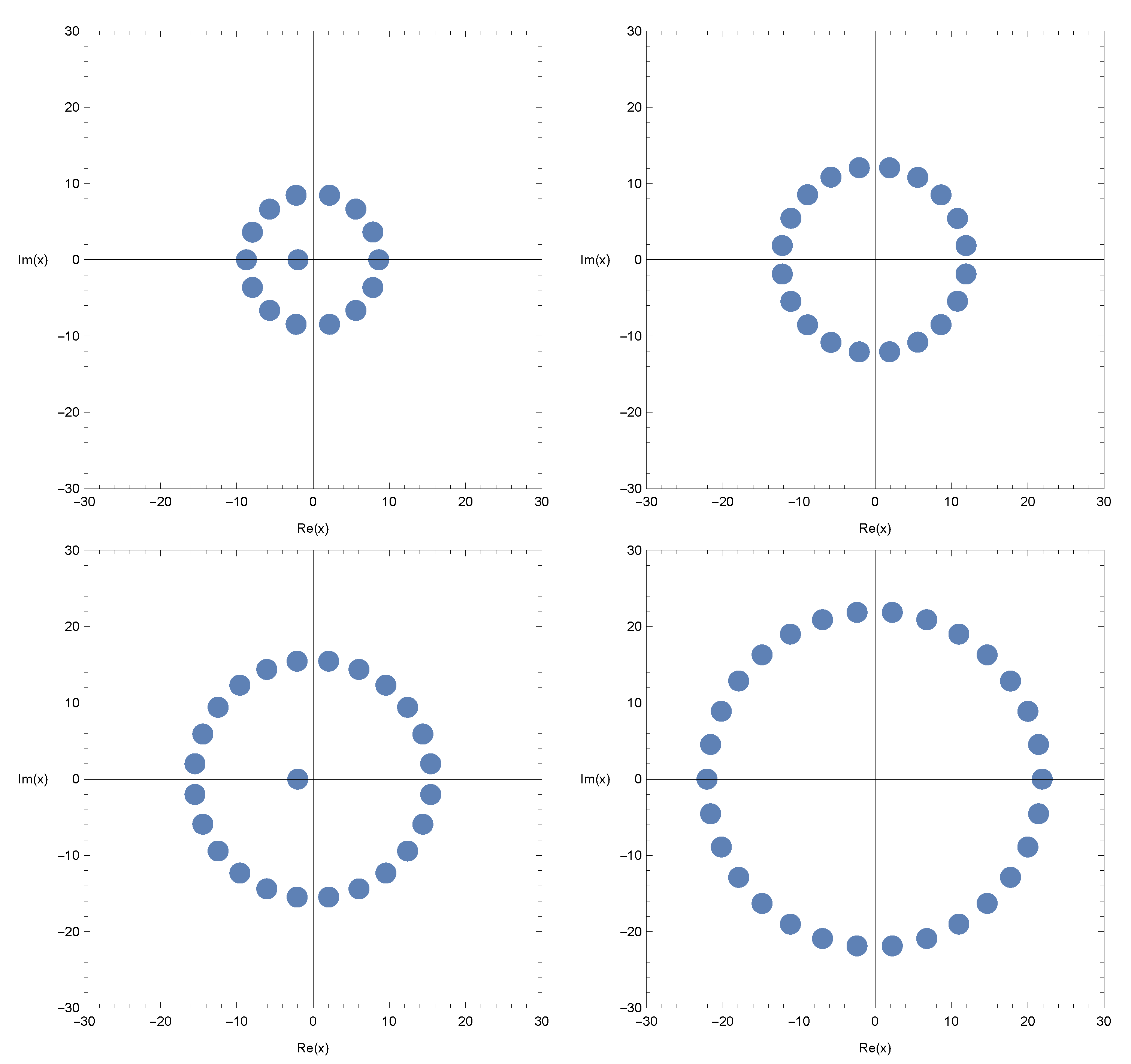
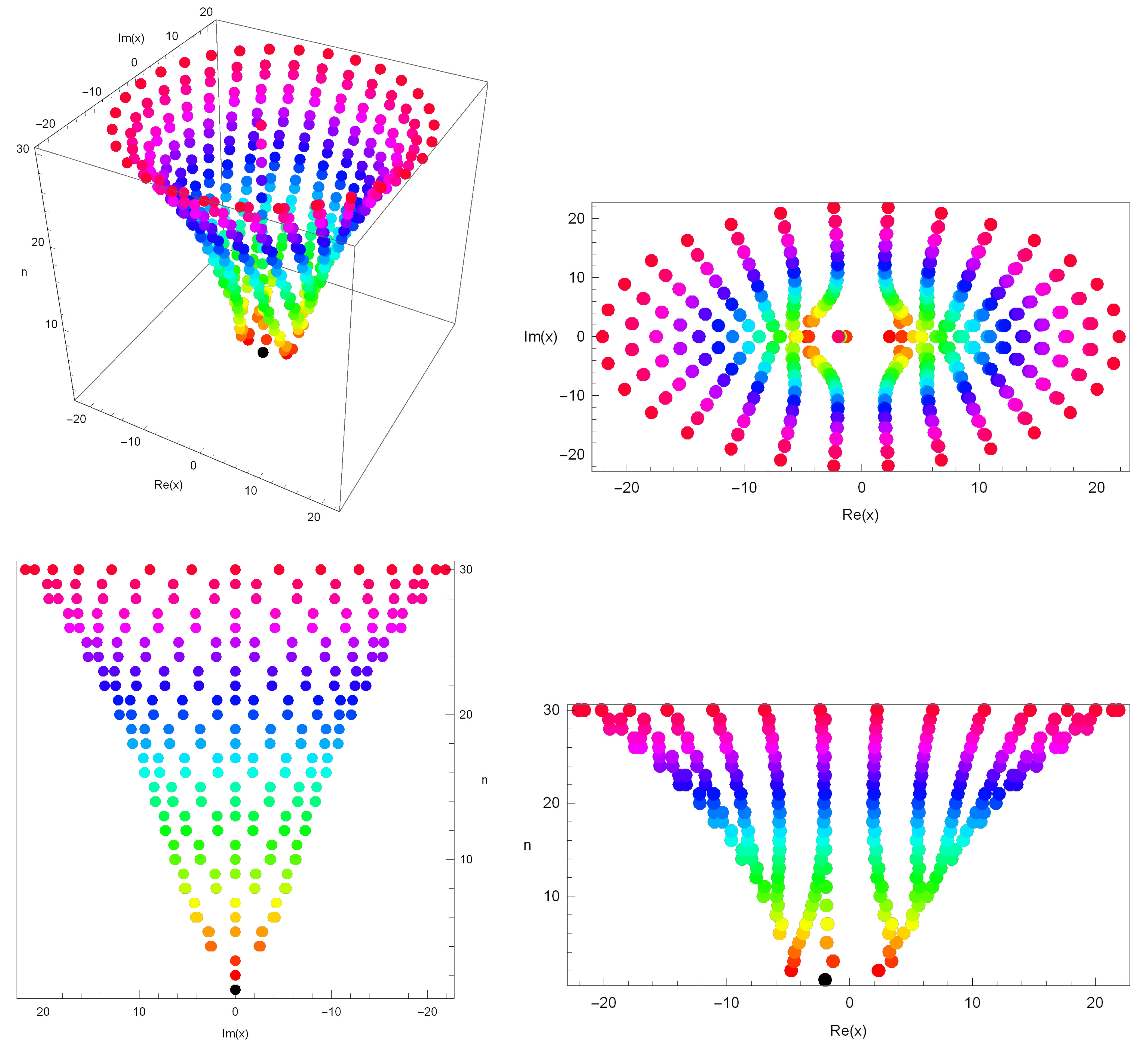
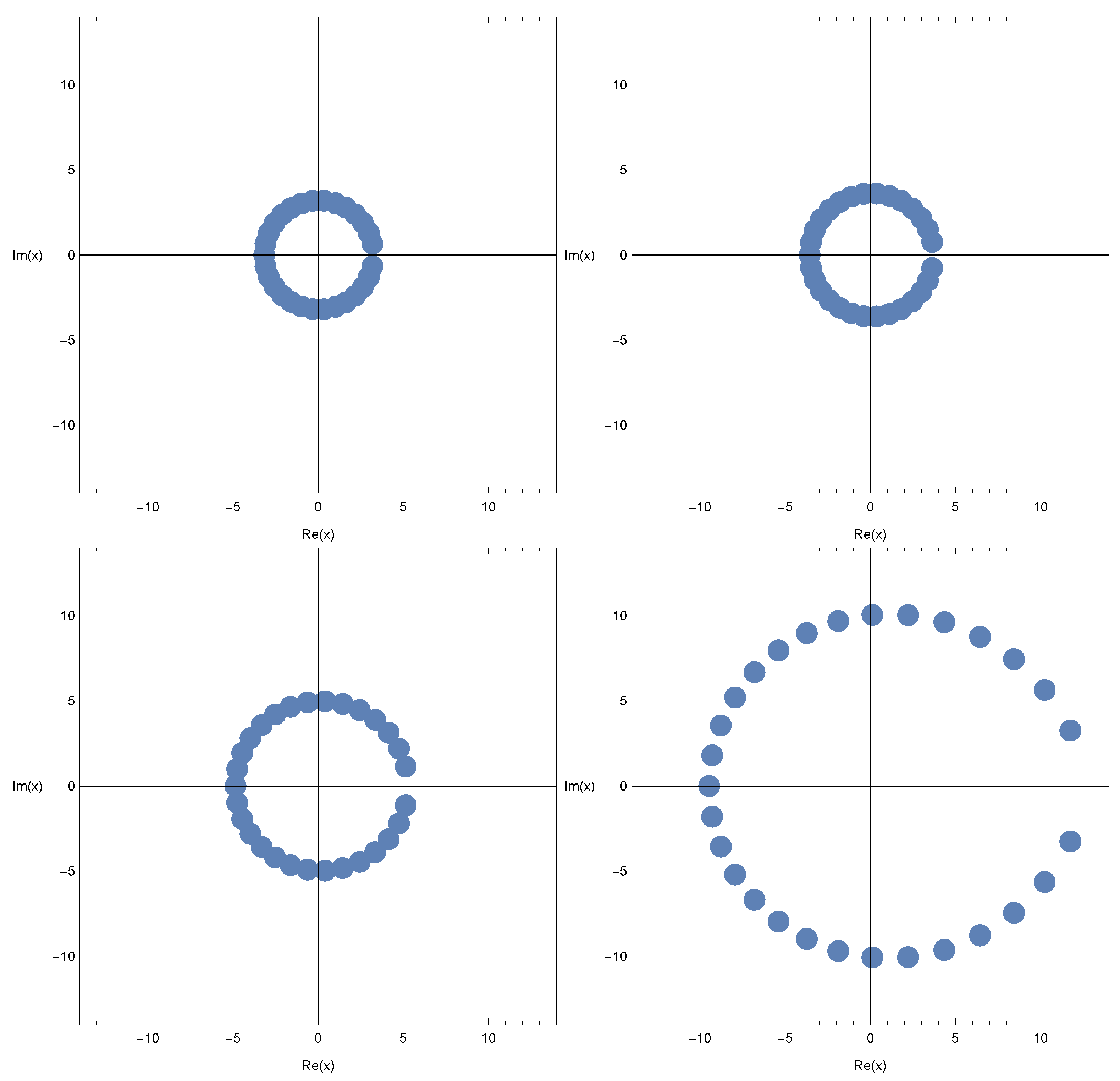
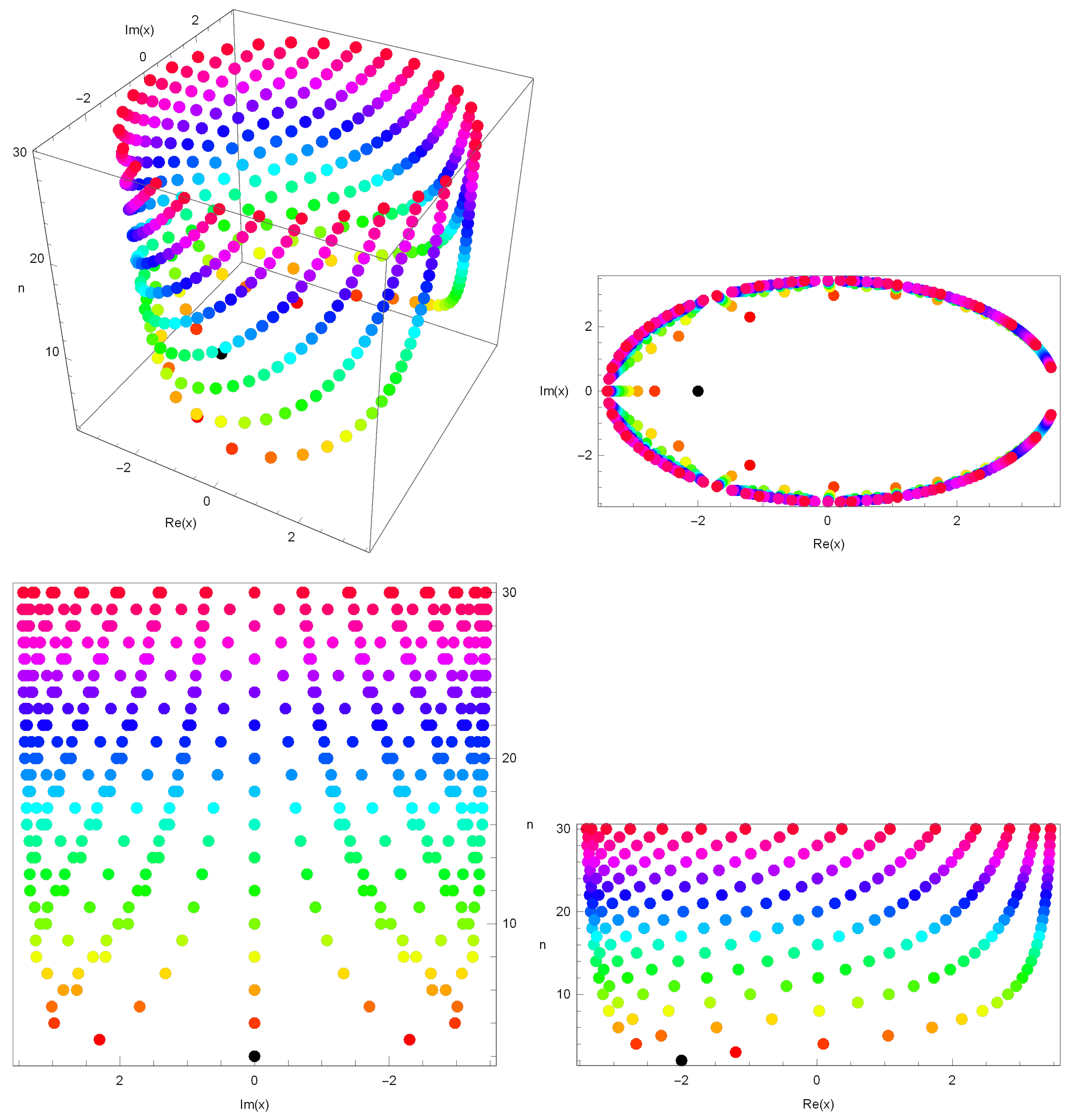
3. New Kinds of -Cosine and -Sine Geometric Polynomials
4. Further Remarks
5. Conclusions
Author Contributions
Funding
Institutional Review Board Statement
Informed Consent Statement
Data Availability Statement
Conflicts of Interest
References
- Duran, U.; Acikgoz, M.; Araci, S. On (p,q)-Bernoulli, (p,q)-Euler and (p,q)-Genocchi polynomials. J. Comput. Theor. Nanosci. 2016, 13, 7833–7908. [Google Scholar] [CrossRef]
- Khan, W.A.; Nisar, K.S.; Baleanu, D. A note on (p,q)-analogue type of Fubini numbers and polynomials. AIMS Math. 2020, 5, 2743–2757. [Google Scholar] [CrossRef]
- Njionou Sadjang, P. On (p, q)-Appell Polynomials. Anal. Math. 2019, 45, 583–598. [Google Scholar] [CrossRef]
- Sadjang, P.N.; Duran, U. On two bivariate kinds of (p,q)-Bernoulli polynomials. Miskolc. Math. Notes 2019, 20, 1185–1199. [Google Scholar] [CrossRef]
- Khan, W.A.; Khan, I.A.; Duran, U.; Acikgoz, M. Apostol type (p,q)-Frobenius Eulerian polynomials and numbers. Afr. Mat. 2021, 32, 115–130. [Google Scholar] [CrossRef]
- Duran, U.; Acikgoz, M. Apostol type (p,q)-Frobenious-Euler polynomials and numbers. Kragujev. J. Math. 2018, 42, 555–567. [Google Scholar] [CrossRef] [Green Version]
- Khan, W.A.; Muhiuddin, G.; Duran, U.; Al-Kadi, D. On (p,q)-sine and (p,q)-cosine Fubini polynomials. Symmetry 2022, 14, 527. [Google Scholar] [CrossRef]
- Ryoo, C.S.; Kang, J.Y. Explicit properties of q-cosine and q-sine Euler polynomials containing symmetric structures. Symmetry 2020, 12, 1247. [Google Scholar] [CrossRef]
- Gupta, V. (p,q)-Baskakov-Kontorovich operators. Appl. Math. Inf. Sci. 2016, 10, 1551–1556. [Google Scholar] [CrossRef]
- Jain, P.; Basu, C.; Panwar, V. On the (p,q)-Mellin transform and its applications. Acta Math. Sci. 2021, 4, 1719–1732. [Google Scholar] [CrossRef]
- Sadjang, P.N. On the fundamental theorem of (p,q)-calculus and some (p,q)-Taylor formulas. Res. Math. 2018, 73, 39. [Google Scholar] [CrossRef]
- Dil, A.; Kurt, V. Investigating geometric and exponential polynomials with Euler-Seidel matrices. J. Integer. Seq. 2011, 14, 1–12. [Google Scholar]
- Kargin, L. Some formulae for products of Fubini polynomials with applications. arXiv 2016, arXiv:1701.01023. [Google Scholar]
- Boyadzhiev, K.N. A series transformation formula and related polynomials. Int. J. Math. Math. Sci. 2005, 23, 3849–3866. [Google Scholar] [CrossRef] [Green Version]
- Tanny, S.M. On some numbers related to Bell numbers. Can. Math. Bull. 1974, 17, 733–738. [Google Scholar] [CrossRef]
- Jamei, M.-M.; Koepf, W. Symbolic computation of some power-trigonometric series. J. Symb. Comput. 2017, 80, 273–284. [Google Scholar] [CrossRef]


| Degree n | x |
|---|---|
| 1 | −2.0000 |
| 2 | |
| 3 | |
| 4 | , |
| , | |
| 5 | , |
| 6 | , |
| 7 | , |
| , 5.0883 | |
| 8 | , |
| , | |
| . |
| Degree n | x |
|---|---|
| 2 | −2.0000 |
| 3 | |
| 4 | |
| 5 | , |
| 6 | , |
| 7 | , |
| , | |
| 8 | , |
| , | |
| 9 | , |
| , | |
| . |
Publisher’s Note: MDPI stays neutral with regard to jurisdictional claims in published maps and institutional affiliations. |
© 2022 by the authors. Licensee MDPI, Basel, Switzerland. This article is an open access article distributed under the terms and conditions of the Creative Commons Attribution (CC BY) license (https://creativecommons.org/licenses/by/4.0/).
Share and Cite
Sharma, S.K.; Khan, W.A.; Ryoo, C.-S.; Duran, U. Diverse Properties and Approximate Roots for a Novel Kinds of the (p,q)-Cosine and (p,q)-Sine Geometric Polynomials. Mathematics 2022, 10, 2709. https://doi.org/10.3390/math10152709
Sharma SK, Khan WA, Ryoo C-S, Duran U. Diverse Properties and Approximate Roots for a Novel Kinds of the (p,q)-Cosine and (p,q)-Sine Geometric Polynomials. Mathematics. 2022; 10(15):2709. https://doi.org/10.3390/math10152709
Chicago/Turabian StyleSharma, Sunil Kumar, Waseem Ahmad Khan, Cheon-Seoung Ryoo, and Ugur Duran. 2022. "Diverse Properties and Approximate Roots for a Novel Kinds of the (p,q)-Cosine and (p,q)-Sine Geometric Polynomials" Mathematics 10, no. 15: 2709. https://doi.org/10.3390/math10152709