Monitoring in a Discrete-Time Nonlinear Age-Structured Population Model with Changing Environment

Abstract

This paper is a contribution to the modeling–methodological development of the application of mathematical systems theory in population biology. A discrete-time nonlinear Leslie-type model is considered, where both the reproduction and survival rates decrease as the total population size increases. In this context, the monitoring problem means that, from the observation of the size of certain age classes as a function of time, we want to recover (estimate) the whole state process (i.e., the time-dependent size of the rest of the classes). First, for the linearization approach, conditions for the existence and asymptotic stability of a positive equilibrium are obtained, then the discrete-time observer design method is applied to estimate an unknown state trajectory near the equilibrium, where we could observe a single age class. It is also shown how the observer design can be used to detect an unknown change in the environment that affects the population dynamics. The environmental change is supposed to be generated by additional dynamics (exosystem). Now, the Leslie-type model is extended with this exosystem, and the observer design is applied to this extended system. In this way, an estimation can be obtained for different (constant or periodic) environmental changes as well.

1. Introduction

The study of monitoring in population systems with tools of mathematical systems theory (MST) looks back to approximately three decades of history. A fundamental monograph on MST, dealing with basic concepts of controllability and observability, was authored by Kalman et al. [1]. By population system, we mean either a) a single population structured in some way, or b) a set of interacting populations. To our knowledge, Varga [2] was the first to apply the concept of observation systems of MST in order to recover the population genetic process from phenotypic observation. A recent continuation of this line of research was shown by Gámez et al. [3]. Later on, this methodology was extended to the monitoring problem of a multispecies community, where, from the observation of certain species (indicators), we wanted to recover (estimate) the state process of the whole community.

For the monitoring of different ecological systems using the observer design methodology of Sundarapandian [4], observer systems have previously been constructed, e.g., in Gámez et al. [5,6]. In particular, in work by López et al. [7], the monitoring of Lotka–Volterra population systems was discussed. A review paper on the different applications of MST in population biology was authored by Varga [8], and somewhat more recent surveys were published by Gámez [9] and Varga et al. [10]. In López et al.’s work [11], by applying a technique of signed digraphs, a new, general approach to the design of a robust observer in continuous-time Lotka–Volterra models was proposed.

All the above references deal with classical continuous-time population models; however, for obvious reasons, in population biology, for practical purposes, discrete-time dynamics models should also be applied. First, in Gámez et al.’s work [12], a discrete-time observer was constructed using the method of Sundarapandian [13].

In the present paper, as a continuation of the above line of research, we adopt the latter observer design method to the monitoring of an age-structured population dynamics model, further developing and extending the initiative commenced by Gődényné Hajdu and Varga [14].

In dynamic population models, both the state and the time may be either discrete or continuous. The classical matrix population models are discrete-state–discrete-time models, where, from the present state, the next state can be obtained by a linear transform.

The use of matrix models to describe the dynamics of an age-structured population goes back to Bernadelli [15], who explained the periodic behavior observed in certain insect populations with a three-dimensional linear dynamic model. The classical discrete-time linear model of an age-specific population growth was introduced by Leslie [16] and further developed by Leslie [17].

We note that in matrix population models, both the state vector and the population projection matrix (PPM, Caswell [18]) describing the linear state transform are non-negative; the dynamics model leaves the non-negative orthant invariant. This property is also characteristic of the linear dynamics models used in economics (see, e.g., Farina and Rinaldi [19]). Therefore, for the study of the asymptotic behavior of such models (including the mathematical demography of human populations; see, e.g., Pianese et al. [20]), the Perron– Frobenius theory of non-negative matrices was applied (see, e.g., Gantmacher [21]), even in the discrete-state—continuous-time case (see, e.g., Varga [22]). Stochastic variants of matrix population models (with environmental or life-cycle stochasticity), involving Markov chains, are discussed in Caswell’s work [18], which is a comprehensive monograph on matrix population models.

The classical discrete-time linear Leslie model of an age-structured population growth, introduced by Leslie [16], would often lead to an unlimited growth, and such behavior is obviously impossible in nature. There are different nonlinearities introduced in the model, implying a more realistic, limited growth. For example, in fisheries, to this end, a (nonlinear) recruitment function was introduced to describe the limited survival of newborn individuals. One of the most popular recruitment functions was due to Beverton and Holt [23] (for further recruitment functions, see Getz and Haight [24] and the recent review by Sharma et al. [25]). We note that a variety of discrete-time density-dependent matrix population models can be obtained by substituting different state dependencies in the different entries of the PPM (see, e.g., Jensen [26]). Further density-dependent matrix population models based on discrete logistic dynamics have been introduced by Liu and Cohen [27]. For a recent overview of both density- and frequency-dependent matrix population models, we again refer to Caswell [18].

In addition to age-specific population models, stage-specific models have also been developed. Since we would like to dedicate another study to the monitoring in stage-structured models (using observer design), in addition to the classical model of Lefkovitch [28], here we only refer to the very recent surveys by Logofet and Salguero-Gómez [29] and Logofet and Ulanova [30] (see also Logofet and Klochkova [31]). Stage-specific models, however, may display structural properties needing different constructions for observer design.

In this study, we consider a nonlinear Leslie-type model, where both the reproduction and the survival rates decrease as the total population size increases (see, e.g., Svirezhev and Logofet [32] and Logofet [33]). In this context, the monitoring problem means that from the observation of the size of certain age class(es) as a function of time, the whole state process (i.e., the time-dependent size of the rest of the age classes) should be recovered (estimated).

The motivation for the present study is the following: In the biological context, it often occurs that only the individuals of certain age class(es) of a population can be observed (i.e., counted). For example, if in biological pest control in a greenhouse we wanted to estimate a pest population of insects, the imagos may be easier to count than other developmental stages (see, e.g., a collection of papers by Schreiber [34] and a recent comprehensive review by Lima et al. [35]). Another practical example occurs in fisheries, where the fish population is estimated from the catch of only individuals over a threshold size. The novelty of the present study is twofold: (a) Although Guiro et al. [36] already applied an observer to estimate the fish stock in a stage-structured population model, their nonlinearity is again based on the above-mentioned Beverton–Holt recruitment function. Our monitoring approach is based, instead, on the nonlinear matrix model of Svirezhev and Logofet [32] cited above, where all vital rates depend on the total population size. (b) In addition to the unknown state process, we also estimate an unknown environmental change affecting the vital rates of the population, which is a new feature of our work with respect to Guiro et al. [36].

The paper is organized as follows: In Section 2, a consistent nonlinear Leslie-type model is defined, with an invariant set as the phase space and conditions for the existence of a unique positive equilibrium of the dynamics. Section 3 is dedicated to a stability analysis. In Section 4, the observer design is illustrated. In Section 5, it is shown how the observer design applies to estimate different (constant and periodic) unknown changes in the environment that affect the population dynamics. A Discussion and Outlook Section closes the main body of the paper.

2. Nonlinear Leslie-Type Model

In this section, we recall some basics of the classical discrete-time, age-structured matrix population model as a starting point of the nonlinear model, for which we propose a monitoring method based on the observer design of MST. Let

$$L_0:=\left[\begin{array}{cccc}\begin{array}{c}{\alpha }_1\\ {\omega }_1\end{array}& \begin{array}{c}{\alpha }_2\\ 0\end{array}& \begin{array}{c}\cdots \\ \cdots \end{array}& \begin{array}{c}\begin{array}{cc}{\alpha }_{n-1}& {\alpha }_n\end{array}\\ \begin{array}{cc}0& \hspace{1em}\hspace{0.33em}0\end{array}\end{array}\\ 0& {\omega }_2& \cdots & \begin{array}{cc}0& \hspace{1em}\hspace{0.33em}0\end{array}\\ ⋮& ⋮& ⋮& \begin{array}{cc}⋮& \hspace{1em}\hspace{0.33em}\hspace{0.33em}⋮\end{array}\\ 0& 0& \cdots & \begin{array}{cc}{\omega }_{n-1}& 0\end{array}\end{array}\right]$$

be a Leslie matrix with reproduction rates ${\alpha }_i\ge 0 \hspace{0.33em}(i=1,\hspace{0.17em}\dots ,\hspace{0.17em}n);\hspace{0.33em}$ survival rates $0<{\omega }_i<1\hspace{0.33em}(i=1,\hspace{0.17em}\dots ,\hspace{0.17em}n-1)$ and state vector

$$x(t)={\left[x_1(t),\hspace{0.17em}{x}_2(t),\hspace{0.17em}\dots ,\hspace{0.17em}{x}_n(t)\right]}^T\hspace{1em}(t=0, 1, 2,\hspace{0.17em}\dots ).$$

Then, the classical Leslie model is

$$x(t+1)=L_{0}x(t)\hspace{1em}(t=0,\hspace{0.17em}\hspace{0.17em}1,\hspace{0.17em}\hspace{0.17em}2,\hspace{0.17em}\dots )$$

with a given non-negative initial state $x(0)\in R_{+0}^n$ (the set of all non-negative vectors of $R^n$).

In the following theorem, based on Svirezhev and Logofet [32], in II. §4 and II. §5, we collected statements from the classical theory of Leslie models, which we needed in the sequel.

Theorem 1.

Let the last age class be reproductive (${\alpha }_n>0$) and either let the first age class be reproductive (${\alpha }_1>0$) or have two consecutive reproductive age classes (${\alpha }_j,\hspace{0.17em}{\alpha }_{j+1}>0$for some$j=2,\hspace{0.17em}\dots ,\hspace{0.17em}n-1$). Then,$L_0$has a unique positive and simple dominant eigenvalue${\lambda }_1>0,$and a unique associated eigenvector$x^{*}>0$with$‖\hspace{0.17em}{x}^{*}‖:={\displaystyle \sum _{i=1}^n{x}_i^{*}}=1$. Furthermore, for any$x(0)>0$, we have$\underset{t\to \infty }{{\displaystyle \lim }}\frac{x(t)}{{\lambda }_1^t}=a{x}^{*}$for some number$a>0$.

In what follows, the conditions of Theorem 1 will be supposed for matrix $L_0$.

Remark 1.

The first condition,${\alpha }_n>0$, implies$L_0$to be irreducible (Section II.4 inSvirezhev and Logofet [32]), while the second one is sufficient but not necessary for$L_0$to be primitive (see Theorem A2.2 in Logofet [33]).

It is known that ${\lambda }_1$ is a kind of long-term growth rate of the population: for ${\lambda }_1$ < 1, the population dies out ($\underset{t\to \infty }{\lim }x(t)=0$), and for ${\lambda }_1$ > 1 the classical Leslie growth is of the Malthus type, $\underset{t\to \infty }{{\displaystyle \lim }}‖x(t)‖=\infty$; in both cases, for t >> 1 we have $x(t+1)\approx {\lambda }_{1}x(t)$. However, in order to avoid unlimited growth, the following modified, nonlinear model was introduced (see, e.g., Logofet [33]).

2.1. Nonlinear Model

For $c>0$, we define

$$\begin{array}{l}{\varphi }_c(x):=\frac{1}{1+c‖x‖}=\frac{1}{1+c{\displaystyle \sum _{i=1}^n{x}_i}},\hspace{1em}{L}_c(x):={\varphi }_c(x)\hspace{0.17em}{L}_0,\\ f_c(x):=L_c(x)\hspace{0.17em}x\hspace{1em}(x\in R_{+0}^n).\end{array}$$

Obviously, in the modified, state-dependent Leslie matrix $L_c(x)$, both the reproduction and the survival rates decrease as the total population size increases. The modified, nonlinear Leslie-type model then was

$$x(t+1)=f_c(x(t))\hspace{1em}(t=0,\hspace{0.17em}\hspace{0.17em}1,\hspace{0.17em}\hspace{0.17em}2,\hspace{0.17em}\dots )$$

(1)

with $x(0)\in R_{+0}^n$ given.

2.2. Equilibrium of the Model

Let us find a nontrivial equilibrium of this dynamics, i.e., a nonzero fixed point of function $f_c$. First, we noted that, with a particular choice of c, the $\hspace{0.17em}{x}^{*}$ from Theorem 1 would be a fixed point of $f_c$. Indeed,

$$f_c(x^{*})=L_c(x^{*})\hspace{0.17em}{x}^{*}={\varphi }_c(x^{*})\hspace{0.17em}{L}_0\hspace{0.17em}{x}^{*}={\varphi }_c(x^{*})\hspace{0.17em}{\lambda }_1{x}^{*}$$

hence,

$$f_c\left(x^{*}\right)=x^{*}\hspace{1em}\iff \hspace{1em}{\varphi }_c\left(x^{*}\right)\cdot {\lambda }_1=1\hspace{1em}\iff \hspace{1em}\frac{1}{1+c‖x^{*}‖}=\frac{1}{{\lambda }_1}\hspace{1em}\iff \hspace{1em}c={\lambda }_1-1.$$

Here, of course, for $c>0,\hspace{1em}{\lambda }_1>1$ should have held. In a more general setting, we had the following:

Theorem 2.

Let the Theorem 1 conditions hold, ${\lambda }_1>1$, and$c>0$be arbitrary. Then,

$$x_c^{*}:=\frac{{\lambda }_1-1}{c}{x}^{*}$$

(2)

is the unique positive equilibrium of dynamics (1).

Proof of Theorem 2.

Substituting $x_c^{*}$, we have

$$f_c(x_c^{*})=\frac{1}{1+c‖x_c^{*}‖}\hspace{0.33em}\frac{{\lambda }_1-1}{c}\hspace{0.33em}{L}_0{x}^{*}=\frac{1}{1+c\hspace{0.33em}\frac{{\lambda }_1-1}{c}}\hspace{0.33em}\frac{{\lambda }_1-1}{c}\hspace{0.33em}{\lambda }_1\hspace{0.33em}{x}^{*}=\frac{{\lambda }_1-1}{c}\hspace{0.33em}{x}^{*}=x_c^{*}.$$

Furthermore, let $x_c^{**}>0$ be an equilibrium for dynamics (1), i.e.,

$$f_c(x_c^{**})={\varphi }_c(x_c^{**})\hspace{0.17em}{L}_0\hspace{0.17em}{x}_c^{**}=x_c^{**}$$

hence,

$$L_0{x}_c^{**}=\frac{1}{{\varphi }_c(x_c^{**})}{x}_c^{**}=(1+c‖x_c^{**}‖)x_c^{**}$$

implying that $1+c‖x_c^{**}‖$ is a positive eigenvalue of $L_0$, associated with eigenvector $x_c^{**}$. Now, using Theorem 1, ${\lambda }_1$ is the unique positive eigenvalue of $L_0$, thus, we have $1+c‖x_c^{**}‖={\lambda }_1$, and, hence, $‖x_c^{**}‖=\frac{{\lambda }_1-1}{c}$. Furthermore, due to the simplicity of eigenvalue ${\lambda }_1$, eigenvector $x_c^{**}$ is a multiple of $x^{*}$. Hence, we obtain $x_c^{**}=‖x_c^{**}‖x^{*}=\frac{{\lambda }_1-1}{c}{x}^{*}$, implying that $x_c^{**}=x_c^{*}$. □

2.3. Invariant Set

Now, we define a phase space (an invariant set) for dynamics (1).

We define

$$M:=\max \left\{{\alpha }_1+{\omega }_1,\hspace{0.33em}{\alpha }_2+{\omega }_2,\hspace{0.33em}\dots ,\hspace{0.33em}{\alpha }_{n-1}+{\omega }_{n-1},\hspace{0.33em}{\alpha }_n\right\},$$

$$S_c:=\left\{\hspace{0.17em}\left.x\in R_{+0}^n\hspace{0.33em}\right|\hspace{1em}‖x‖\le \frac{M}{c}\right\}.$$

Theorem 3.

For any$c>0$, set$S_c$is invariant under$f_c$.

Proof of Theorem 3.

Let $x\in S_c$. Then,

$$‖f_c(x)‖=\frac{1}{1+c\hspace{0.33em}‖x‖}‖\left[\begin{array}{c}{\alpha }_1{x}_1+{\alpha }_2{x}_2+\dots +{\alpha }_n{x}_n\\ {\omega }_1{x}_1\\ {\omega }_2{x}_2\\ \begin{array}{c}⋮\\ {\omega }_{n-1}{x}_{n-1}\end{array}\end{array}\right]‖$$

$$=\frac{{\alpha }_1{x}_1+{\alpha }_2{x}_2+\dots +{\alpha }_n{x}_n+{\omega }_1{x}_1+\dots +{\omega }_{n-1}{x}_{n-1}}{1+c\hspace{0.33em}‖x‖}$$

$$=\frac{\left({\alpha }_1+{\omega }_1\right)x_1+\left({\alpha }_2+{\omega }_2\right)x_2+\dots +\left({\alpha }_{n-1}+{\omega }_{n-1}\right)x_{n-1}+{\alpha }_n{x}_n}{1+c\hspace{0.33em}‖x‖}$$

$$\le \frac{M{x}_1+M{x}_2+\dots +M{x}_{n-1}+M{x}_n{}_{}}{1+c\hspace{0.33em}‖x‖}=\frac{M‖x‖}{1+c‖x‖}\le \frac{M}{c}.$$

□

Remark 2.

Since$S_c$is convex and compact, and$f_c$is continuous, the Brouwer fixed-point theorem would imply that$f_c$has a fixed point in$S_c$. Nevertheless,$x=0\in S_c$is always a trivial fixed point. Of course, we are interested in a nontrivial equilibrium of dynamics (1).

Now, in terms of the demographic parameters ${\alpha }_i$ and ${\omega }_i$, we find a necessary and sufficient condition for equilibrium $x_c^{*}$ to belong to the invariant set $S_c$. It is known (Logofet [33]) that the normed characteristic equation of $L_0$ is

$${\lambda }^n-{\alpha }_1{\lambda }^{n-1}-{\alpha }_2{\omega }_1{\lambda }^{n-2}-\dots -{\alpha }_n{\omega }_1\cdots {\omega }_{n-1}=0.$$

Hence, it is easy to see that a $\lambda >0$ is an eigenvalue of $L_0$ if, and only if,

$$q(\lambda ):=\frac{{\alpha }_1}{\lambda }+\frac{{\alpha }_2{\omega }_1}{{\lambda }^2}+\dots +\frac{{\alpha }_n{\omega }_1\cdots {\omega }_{n-1}}{{\lambda }^n}=1.$$

(3)

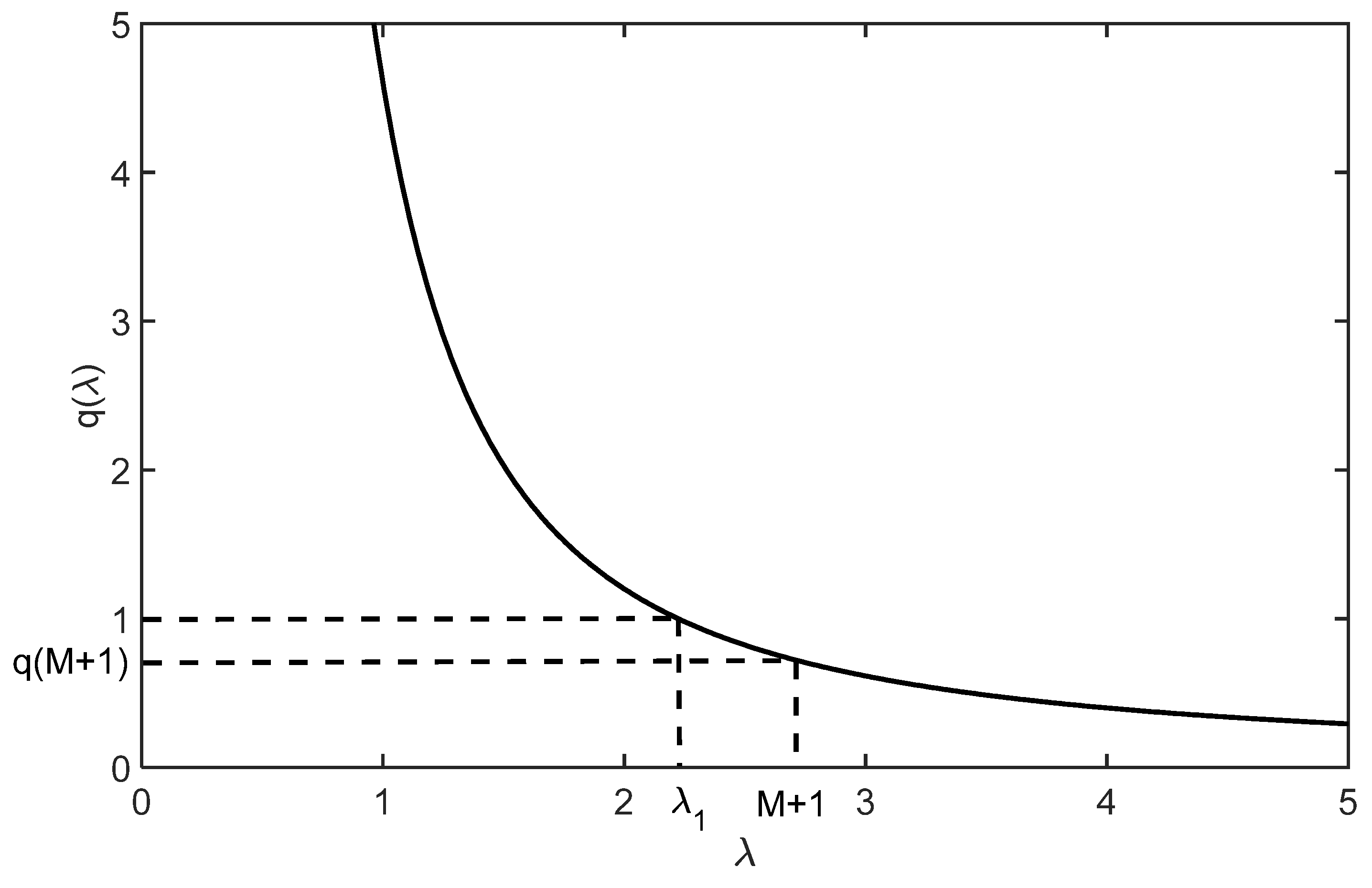
Furthermore, since function $q$ is strictly decreasing, with $\underset{\lambda \to +0}{\lim }q(\lambda )=\infty$ and $\underset{\lambda \to \infty }{\lim }q(\lambda )=0$, condition

$$x_c^{*}\in S_c$$

(4)

holds if, and only if,

$$\frac{{\lambda }_1-1}{c}\le \frac{M}{c}\iff {\lambda }_1\le M+1\iff q(M+1)\le 1$$

(see Figure 1).

Hence, we have the following

Theorem 4.

Under the conditions of Theorem 1,$x_c^{*}\in S_c$if, and only if, for function q defined in (3), we have

$$q(M+1)\le 1$$

(5)

Example 1.

Let us consider the simplified case, when all demographic parameters are the same:${\alpha }_1=\dots ={\alpha }_n=\alpha$,${\omega }_1={\omega }_2=\dots ={\omega }_{n-1}=\omega$. Then,

$$M=\max \left\{\alpha +\omega ,\hspace{0.33em}\alpha +\omega ,\hspace{0.33em}\dots ,\hspace{0.33em}\alpha +\omega ,\hspace{0.33em}\alpha \right\}=\alpha +\omega .$$

Therefore,

$$\begin{array}{ll}& q\left(M+1\right)=q\left(\alpha +\omega +1\right)=\frac{\alpha }{\alpha +\omega +1}+\frac{\alpha \omega }{{(\alpha +\omega +1)}^2}+\dots +\frac{\alpha {\omega }^{n-1}}{{(\alpha +\omega +1)}^n}\\ & =\frac{\alpha }{\alpha +\omega +1}\left(1+\frac{\omega }{\alpha +\omega +1}+\dots +\frac{{\omega }^{n-1}}{{(\alpha +\omega +1)}^{n-1}}\right)\le \frac{\alpha }{\alpha +\omega +1}{\displaystyle {\displaystyle \sum }_{k=0}^{\infty }}{\left(\frac{\omega }{\alpha +\omega +1}\right)}^k\\ & =\frac{\alpha }{\alpha +\omega +1}\frac{1}{1-\frac{\omega }{\alpha +\omega +1}}=\frac{\alpha }{\alpha +1}.\end{array}$$

Thus, inequality (5) was satisfied, implying that equilibrium$x_c^{*}$belongs to the interior of the phase space$S_c$. This example also implies an infinite family of examples. Indeed, by the continuity of function$q$, the above strict inequality also holds for all models having different demographic parameters${\alpha }_i$and${\omega }_i$, sufficiently near the particular values$\alpha$and$\omega$of the above example.

Remark 3.

Since, in the above reasoning, inequality (5) is strictly satisfied, and$x^{*}>0$, we can also conclude that in Example 1,$x_c^{*}$also belongs to the interior of the invariant set$S_c$. Through continuity reasoning, it also follows that for any parameter set for${\alpha }_i$and${\omega }_i$close to that of Example 1,$x_c^{*}$also belongs to the interior of$S_c$.

3. Stability of the Positive Equilibrium

For the sake of simplicity, we consider the case of $n=3$. Now, with a given $c>0$, dynamics (1) is considered with

$$L_0:=\left[\begin{array}{ccc}{\alpha }_1& {\alpha }_2& {\alpha }_3\\ {\omega }_1& 0& 0\\ 0& {\omega }_2& 0\end{array}\right].$$

In order to satisfy the conditions of Theorem 1, we suppose that ${\alpha }_3>0,$ and at least one of the inequalities ${\alpha }_1>0$ or ${\alpha }_2>0$, holds. Assuming that ${\lambda }_0>1$, with Theorem 2 we obtain that

$$x_c^{*}:=\frac{{\lambda }_0-1}{c}{x}^0$$

is the unique positive equilibrium of dynamics (1). Therefore, the Jacobian matrix at this positive equilibrium is

$$f_c^{\prime }(x_c^{*})=L_c(x)-\frac{c}{{\left(1+c‖x_c^{*}‖\right)}^2}\cdot \left[\begin{array}{ccc}{L}_0{x}_c^{*}& L_0{x}_c^{*}& L_0{x}_c^{*}\end{array}\right].$$

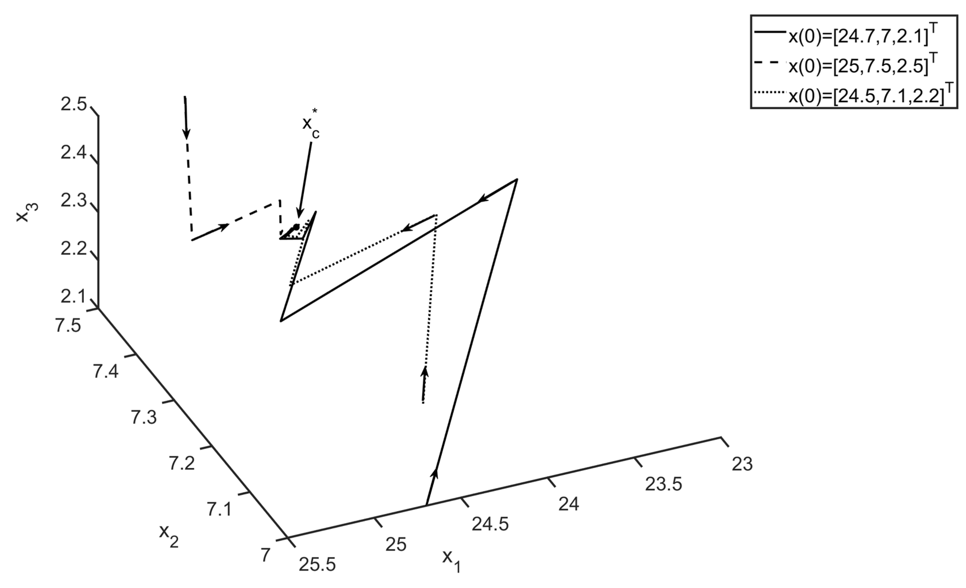
The following example illustrates the stability of the population age structure.

Example 2.

Consider a population with the following demographic parameters:

${\alpha }_1=0,{\alpha }_2=6,{\alpha }_3=10,{\omega }_1=0.8,{\omega }_2=0,9$, and set c = 0.05.

Conditions of Theorem 1 were fulfilled, so matrix $L_0$ has a unique positive and simple dominant eigenvalue ${\lambda }_1=2.73>1$ and the unique normed eigenvector associated with it is $x^{*}={[0.72, 0.21, 0.07]}^{\mathrm{T}}$ (with $‖x^{*}‖=x_1+x_2+x_3=1$).

The unique positive equilibrium of dynamics (1) is $x_{\mathrm{c}}^{*}={[24.9, 7.3, 2.4]}^{\mathrm{T}}$. Moreover, since $M=\max \{{\alpha }_1+{\omega }_1,{\alpha }_2+{\omega }_2,{\alpha }_3\}=10$, we have $‖x_c^{*}‖=34.6<200=\frac{M}{c}$. Therefore, $x_c^{*}\in S_c$. The eigenvalues of the Jacobian at equilibrium, $A:=f_c^{\prime }(x_c^{*})$, are: $0.5\pm 0.32i$, 0.37. Therefore, A has a spectral radius of less than one (i.e., only has eigenvalues with modulus of less than one) and, hence, equilibrium $x_c^{*}$ is asymptotically stable. In Figure 2, we can see how the solution of system (1) converge to $x_c^{*}$ for different initial conditions.

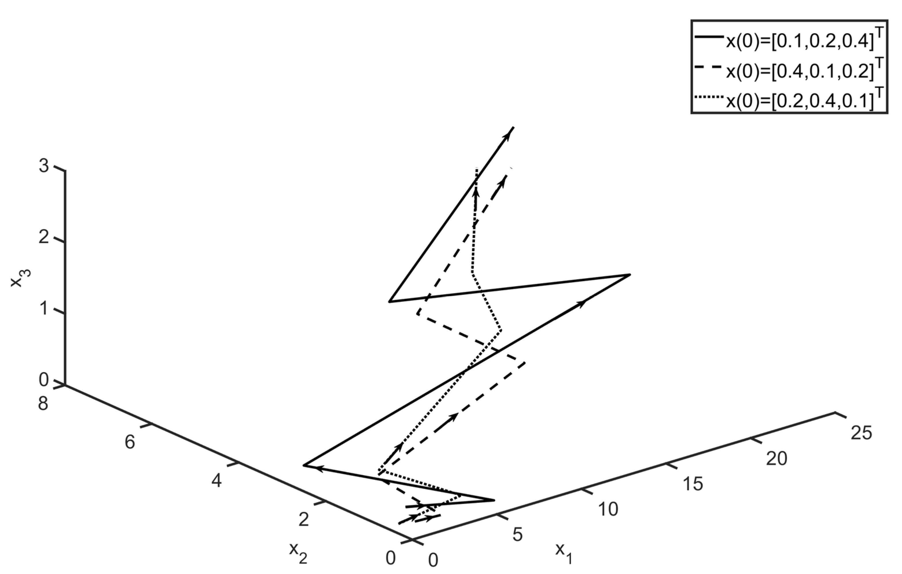
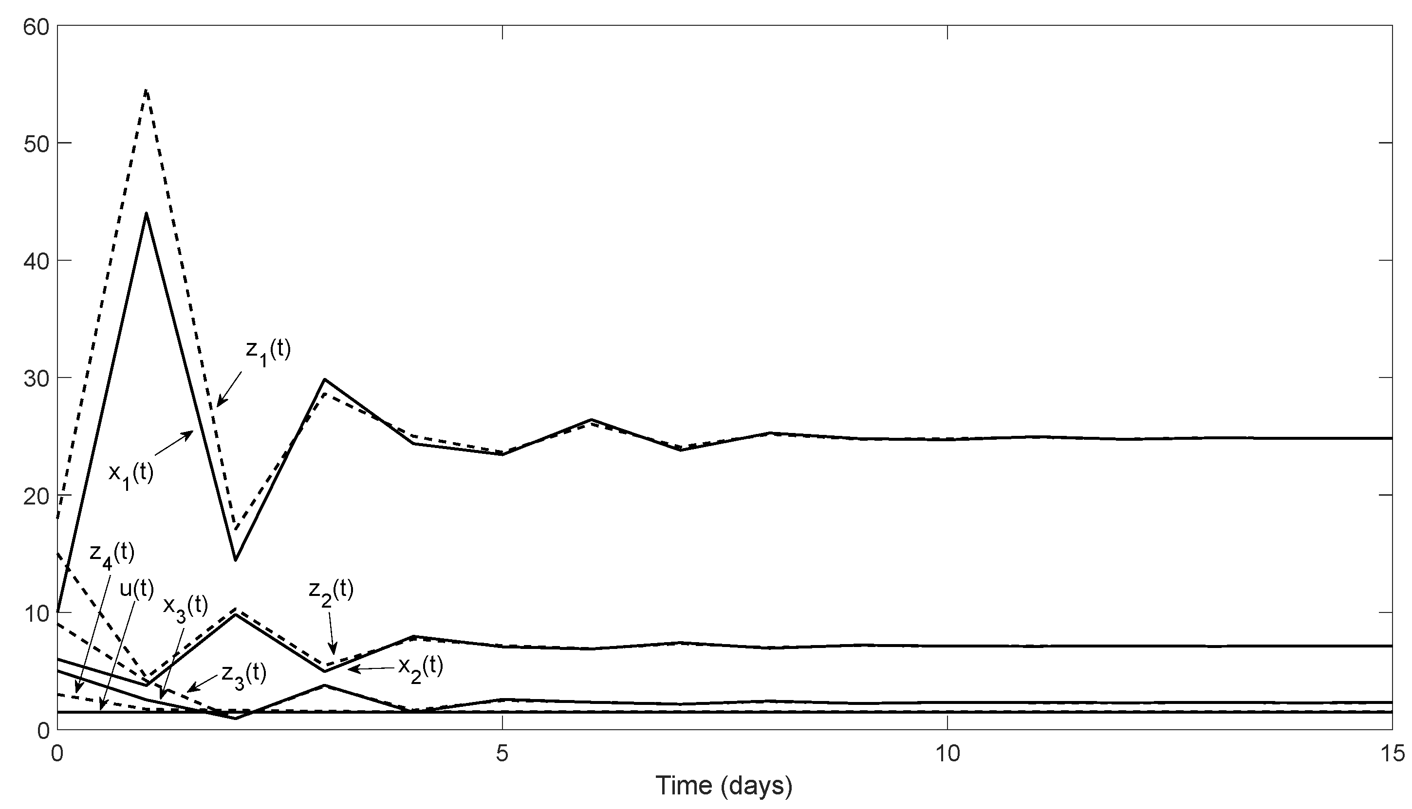
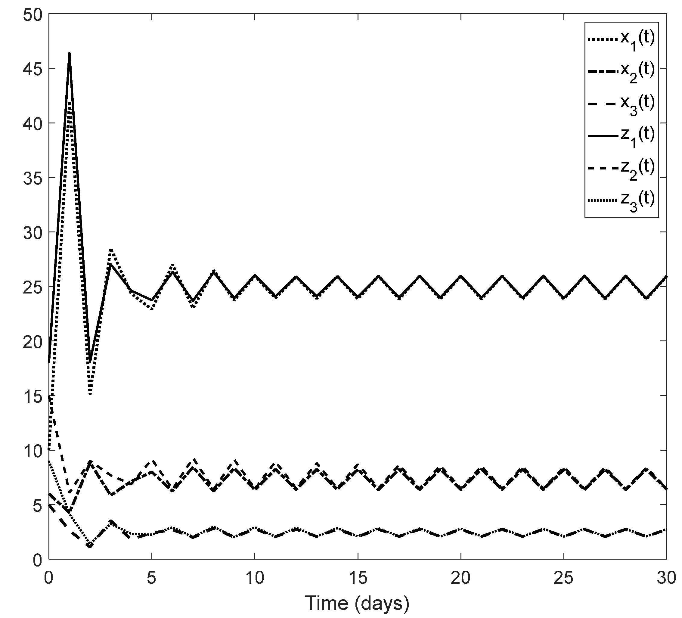
Remark 4.

For the zero equilibrium, we have$f_c^{\prime }(0)=L(0)$, and since, in our case,${\lambda }_1>1$, the zero equilibrium is unstable. For our Example 1, inFigure 3, it is shown how the solutions of system (1) initially near zero diverge from zero (In fact, the eigenvalues of$f_c^{\prime }(0)$are$2.73, -1.36\pm 0.88\mathrm{i}$).

4. Construction of a Local Observer

4.1. Observability of the System: Observing the Second Age Class

Consider the observation system consisting of dynamics (1),

$$x(t+1)=f_c(x(t))\hspace{1em}(t=0,\hspace{0.17em}1,\hspace{0.17em}2,\hspace{0.17em}\dots ),$$

(6)

and the observed function

$$y(t)=h(x(t))=x_2(t)-x_{c2}^{*}.$$

(7)

Then, $y(t)=C(x(t)-x_c^{*})$, where $C:=h^{\prime }(x_c^{*})=\left(\begin{array}{ccc}0& 1& 0\end{array}\right)$, and $h(x_c^{*})=0$.

Now, an observation system is said to be locally observable near an equilibrium, if there exists a vicinity of this equilibrium where different state processes provide different observations.

Theorem 5.

If${\alpha }_2\le {\alpha }_3$, then observation system (6)–(7) is locally observable near the equilibrium$x_c^{*}$.

Proof of Theorem 5.

According to the basic theorem on observability (see, e.g., Sundarapandian [12]) it is enough to see that with matrix $A:=f_c^{\prime }(x_c^{*})$, we have $\mathrm{rank}\left[\begin{array}{c}C\\ CA\\ C{A}^2\end{array}\right]=3$. We easily obtain that

$$\det \left[\begin{array}{c}C\\ CA\\ C{A}^2\end{array}\right]=-\frac{{\omega }_1^2\left[c\left(c{\omega }_2{x}_{c1}^{*}+{\alpha }_2\left(-1-c‖x_c^{*}‖+c{x}_{c1}^{*}\right)\right)x_{c2}^{*}+{\alpha }_3\left(1+c\left(‖x_c^{*}‖-1\right)\right)\left(1+c\left(‖x_c^{*}‖-x_{c1}^{*}-x_{c3}^{*}\right)\right)\right]}{{\left(1+c‖x_c^{*}‖\right)}^5}.$$

Since $‖x^{*}‖=1$ and ${\lambda }_1>1$, we have $x_c^{*}=\frac{{\lambda }_1-1}{c}{x}^{*}\Rightarrow x_c^{*}=\frac{{\lambda }_1-1}{c}>0$. Now, from $x_{c1}^{*}=‖x_c^{*}‖x_1^{*},\hspace{1em}{x}_{c2}^{*}=‖x_c^{*}‖x_2^{*},\hspace{1em}{x}_{c3}^{*}=‖x_c^{*}‖x_3^{*},$ we obtain that $\det \left[\begin{array}{c}C\\ CA\\ C{A}^2\end{array}\right]$ is equal to

$$-\frac{{\omega }_1^2\left[c‖x_c^{*}‖\hspace{0.17em}\left[{\alpha }_2\left(-1+c‖x_c^{*}‖\hspace{0.17em}\left(-1+x_1^{*}\right)\right)+c‖x_c^{*}‖{\omega }_2{x}_1^{*}\right]x_2^{*}+{\alpha }_3\left(-1+c‖x_c^{*}‖\hspace{0.17em}\left(-1+x_1^{*}\right)\right)\left(-1+c‖x_c^{*}‖\hspace{0.17em}\left(-1+x_1^{*}+x_3^{*}\right)\right)\right]}{{\left(1+c‖x_c^{*}‖\right)}^5}.$$

Regrouping terms, we have that $\det \left[\begin{array}{c}C\\ CA\\ C{A}^2\end{array}\right]$ is equal to

$$-\frac{{\omega }_1^2\left[c^2{‖x_c^{*}‖}^2{\omega }_2{x}_1^{*}{x}_2^{*}+\hspace{0.17em}\left[-1+c‖x_c^{*}‖\hspace{0.17em}\left(-1+x_1^{*}\right)\right]\cdot \left[c‖x_c^{*}‖{\alpha }_2{x}_2^{*}-{\alpha }_3+{\alpha }_{3}c‖x_c^{*}‖\left(-1+x_1^{*}+x_3^{*}\right)\right]\right]}{{\left(1+c‖x_c^{*}‖\right)}^5}.$$

Since ${\alpha }_2\le {\alpha }_3$, $‖x_c^{*}‖>0,\hspace{1em}$ and $‖x_{}^{*}‖=1$, we have that $-1+x_1^{*}<0$ and $-1+x_1^{*}+x_3^{*}=-x_2^{*}$, implying $\det \left[\begin{array}{c}C\\ CA\\ C{A}^2\end{array}\right]<0$. Therefore, observation system (6)–(7) is locally observable near the positive equilibrium. □

4.2. Construction of a Local Observer: Observing the Second Age Class

We illustrate the observer design with the following:

Example 3.

We use the same parameters as in Example 2. Observing$x_2(t)$, as${\alpha }_2\le {\alpha }_3$, and applying Theorem 5, we obtain that observation system (6)–(7) is locally observable near equilibrium$x_c^{*}={[24.9, 7.3, 2.4]}^T$. Now, we shortly quote some basics of observers from Sundarapandian [13].

Consider a general discrete-time observation system

$$x(t+1)=f(x(t))\hspace{1em}(t=0,\hspace{0.17em}1,\hspace{0.17em}2,\hspace{0.17em}\dots )$$

(8)

$$y(t)=h(x(t))$$

(9)

with an equilibrium $x_{}^{*}$, where h vanishes. Denoted by A and C the Jacobian of f and h at $x_{}^{*}$, respectively, suppose that K is a matrix of appropriate size, such that $A-KC$ has a spectral radius of less than one. Then,

$$z(t+1)=f(z(t))+K(y(t)-h(z(t)))$$

(10)

is a local exponential observer for system (8) and (9) in the following sense:

(a)

$x\left(0\right)=z\left(0\right) \mathrm{implies} x\left(t\right)=z\left(t\right) \left(t=1,2,3,\dots \right)$.

(b)

For $x\left(0\right) \mathrm{and} z\left(0\right)$ close enough to $x_{}^{*}$, for some M > 0 and 0 < a < 1, we have

$$‖z(t)-x(t) ‖\le M{a}^t (t=1,\hspace{0.17em}2,\hspace{0.17em}3,\dots ).$$

Remark 5.

The intuitive interpretation of the constructed observer system (10) is the following: Instead of the unknown initial value$x(0)$, we start the original recursion (8) with an arbitrary initial value$z(0)$near the equilibrium, but with an additional correction term$K(y(t)-h(z(t)))$. The fact that, for the auxiliary matrix$K$, all the eigenvalues of$A-KC$are less than one in modulus implies that the known solution$z(t)$of the observer system (10) approaches the unknown state process$x(t)$at an exponential rate.

Back to our Example 3, in fact, for $K=\left[\right(1,\hspace{0.17em}0,\hspace{0.17em}{0\left)\right]}^T$, matrix $A-KC$ had the following eigenvalues: $-0.46\pm 0.45\mathrm{i}$, 0.45. Hence, $A-KC$ has a spectral radius of less than one, and Equation (10) provides the following observer system for system (8) and (9):

$$\left.\begin{array}{l} \begin{array}{l}{z}_1(t+1)=\frac{1}{1+0.05‖z(t)‖}\left(6z_2(t)+10z_3(t)+\left(x_2(t)-z_2(t)\right)\right),\\ z_2(t+1)=\frac{1}{1+0.05‖z(t)‖}0.8z_1(t),\\ z_3(t+1)=\frac{1}{1+0.05‖z(t)‖}0.9z_2(t).\end{array}\end{array}\right\}$$

(11)

In Figure 4, it is shown how the solution of observer (11) with an initial value $z(0){=\left[\right(18, 15, 9]}^T$ approaches the solution of the original system, with an initial value x(0) = [10, 6, 5]^T, considered as the “unknown solution” of (6).

5. Construction of an Observer System with Environmental Change

Now, we show how the above observer design methodology could be used to estimate certain changes in population parameters due to abiotic environmental effects. In general, this time-dependent change could be described as an additive term u(t), generated by its own dynamics, called the exosystem. Here, additivity means that a model parameter changed from $\alpha$ to $\alpha +u(t)$.

5.1. Constant Environmental Change Affecting a Reproduction Rate

Example 4.

For an illustration of this idea, let us consider our Leslie-type model with parameter values of Example 2:${\alpha }_1=0,{\alpha }_2=6,{\alpha }_3=10,{\omega }_1=0.8,{\omega }_2=0.9$, c = 0.05, and suppose that there is an additive change u(t) in the reproduction rate of the third age class.

$$\left.\begin{array}{l} \begin{array}{l}{x}_1(t+1)=\frac{1}{1+c‖x(t)‖}\left(6x_2(t)+(10+u(t))x_3(t)\right),\\ x_2(t+1)=\frac{1}{1+c‖x(t)‖}0.8x_1(t),\\ x_3(t+1)=\frac{1}{1+c‖x(t)‖}0.9x_2(t).\\ u(t+1)=u(t);\end{array}\end{array}\right\}$$

(12)

$$y(t)=h(x(t),u)=x_2(t)-x_{c2}^{*}.$$

(13)

Here, the last equation of system (12) models the exosystem, which, in the present case, describes that the reproduction rate ${\alpha }_3$ changes to an unknown constant. Observation (13) is the same as in Example 3. The construction of an observer system will be based on Sundarapandian’s work [13], applying the observer design to the extended system (12) and (13), denoted by $F(x,u)$ the right-hand side of system (12). Since $x_c^{*}$ is an asymptotically stable equilibrium for the original system, and 0 is a stable equilibrium for the exosystem, with the discrete-time adaptation of a result by Isidori [37], we obtain that $(x_c^{*},\hspace{0.33em}0)$ is a stable equilibrium of system (12). Following Sundarapandian [13], for the linearization, we calculated the Jacobian $A:=F^{\prime }(x_c^{*},\hspace{0.33em}0)$ and $C:=\left[\begin{array}{ccc}0& 1& 0\end{array} 0\right]$, and with an auxiliary matrix $K:={\left[\begin{array}{ccc}1& 0& 0\end{array} 0.14\right]}^T$, we obtain that $A-KC$ has a spectral radius of less than one. Hence, we obtain the following observer system for system (12) and (13):

$$\left.\begin{array}{l} \begin{array}{l}{z}_1(t+1)=\frac{1}{1+0.05‖z(t)‖}\left(6z_2(t)+(10+z_4(t))z_3(t)\right)+(x_2(t)-z_2(t)),\\ z_2(t+1)=\frac{1}{1+0.05‖z(t)‖}0.8z_1(t),\\ z_3(t+1)=\frac{1}{1+0.05‖z(t)‖}0.9z_2(t),\\ z_4(t+1)=z_4(t)+0.14(x_2(t)-z_2(t)) . \end{array}\end{array}\right\}$$

(14)

The interpretation of observer system (14) is shown in Figure 5.

5.2. Periodic Environmental Change in a Survival Rate

Suppose that survival rate ${\omega }_1$ changes periodically due to an environmental (e.g., seasonal) change.

Therefore, we fix

$$0<\delta <\min \{{\omega }_1,1-{\omega }_1\}.$$

(15)

Then, ${\omega }_1+\delta u_1(t)\in [0, 1]$, whenever $u_1(t)\in [-1, 1]$ (t = 0, 1, 2,…). Therefore, the following is a consistent population model with a periodically changing survival rate of the second age class:

$$\left. \begin{array}{l}{x}_1\left(t+1\right)=\frac{1}{1+cx\left(t\right)}\left({\alpha }_1{x}_1\left(t\right)+{\alpha }_2{x}_2\left(t\right)+{\alpha }_3{x}_3\left(t\right)\right),\\ x_2\left(t+1\right)=\frac{1}{1+cx\left(t\right)}\left({\omega }_1+\delta u_1\left(t\right)\right)x_1\left(t\right),\\ \hspace{1em}\hspace{1em}{x}_3\left(t+1\right)=\frac{1}{1+cx\left(t\right)}{\omega }_2{x}_2\left(t\right),\end{array}\right\}$$

(16)

$$u_1\left(t+2\right)=u_1\left(t\right).$$

(17)

In order to handle the observer design in the standard form, we needed to transform the second-order discrete-time dynamics to the equivalent first-order two-dimensional system. With notation $u_2(t):=u_1(t+1)$, $u(t):=\left[\begin{array}{c}{u}_1(t)\\ u_2(t)\end{array}\right]$ and $B:=\left[\begin{array}{cc}0& 1\\ 1& 0\end{array}\right]$, the exosystem corresponding to (17) is

$$u(t+1)=Bu(t) (t=0, 1, 2,\dots )$$

(18)

Since, for any $\epsilon \in [0,1]$, the solution of system (18) with initial conditions $u(0):=\left[\begin{array}{c}\epsilon \\ -\epsilon \end{array}\right]$ is

$$u(t)={(-1)}^{t}u(0) (t=0, 1, 2,\dots ),$$

$u^{\ast }:=\left[\begin{array}{c}0\\ 0\end{array}\right]$ is a stable equilibrium of system (18).

Example 5.

Continuing with parameters of the previous Example 4, we know that$x_c^{*}={\left[\begin{array}{ccc}24.9& 7.3& 2.4\end{array}\right]}^T$is an asymptotically stable equilibrium of system (16) with$\delta =0$.

Similarly to Example 4, we obtain that $\left[\begin{array}{c}{x}_c^{*}\\ u^{\ast }\end{array}\right]$ is a stable equilibrium of the extended system given by (16) and (18). According to condition (15), we can choose, for example, $\delta :=0.15$.

For an illustration, let us assume again that the second age class is observed:

$$y(t)=h(x(t),u(t))=x_2(t)-x_{c2}^{*},$$

(19)

and we want to recover $x(t)$ and $u(t)$, considered to be unknown.

According to Sundarapandian [13], we linearize calculating the Jacobians $A:=F^{\prime }(x_c^{*},u^{\ast })$ and $C:=\left[\begin{array}{ccc}0& 1& 0\end{array} 0\right]$. It is easily checked with matrix $K:={\left[\begin{array}{ccc}1& 0& 0\end{array} 0.14\right]}^T$ that the resulting matrix $A-KC$ has a spectral radius of less than one. Now, the observer design provides the following observer system for system (16)–(19):

$$\left.\begin{array}{l}{z}_1(t+1)=\frac{1}{1+0.05‖z(t)‖}\left(6z_2(t)+10z_3(t)\right)+\left(x_2(t)-z_2(t)\right),\\ z_2(t+1)=\frac{1}{1+0.05‖z(t)‖}\left(0.8+0.15z_4(t)\right)\hspace{0.17em}{z}_1(t),\\ \begin{array}{l}\hspace{1em}\hspace{1em}{z}_3(t+1)=\frac{1}{1+0.05‖z(t)‖}0.9z_2(t),\\ \hspace{1em}\hspace{1em}{z}_4(t+1)=z_5(t)+0.14\left(x_2(t)-z_2(t)\right),\\ \hspace{1em}\hspace{1em}{z}_5(t+1)=z_4(t).\end{array}\end{array}\right\}$$

(20)

In Figure 6 and Figure 7, we can see how the solution of observer (20) with the initial value $z(0)={[18 15 9 2 1 ]}^T$ approached the “unknown” state process and the periodic environmental change, with an initial value of $\left[\begin{array}{c}x(0)\\ u(0)\end{array}\right]={[10 6 5 0.5 -0.5]}^T$.

6. Discussion and Outlook

First of all, we note that Gámez et al. [6] already proposed the observer approach to the deterministic stock estimation of a single fish population with reserve area, which obeyed the continuous-time logistic dynamics. The discrete-time observer approach to monitoring, proposed in the present paper (also including the case of a changing environment), is different from that considered by Ngom et al. [38]. Indeed, in the latter, the first age class was governed by a Beverton–Holt recruitment function and the time-dependent survival rates (including a time-dependent fishing effort) were supposed, while there is a feedback of the total population size, both in the reproduction and the survival rates in our model.

Instead of an age-classified population, it is also natural to divide the individuals of the considered population into groups, according to their developmental stages. For such stage-specific population models applied in biological pest control, see, e.g., Garay et al. [39]. Therefore, for both the theory and the possible applications, it is a further promising challenge to extend the monitoring methodology developed in the present paper, to stage-structured population models. While in the age-specific model all surviving individuals pass to the next age class in unite time, a part of the surviving individuals may have remained in the same stage in the stage-specific model, resulting in a different dynamic model. Guiro et al. [36] already applied an observer to estimate fish stock in a stage-structured population model, but the nonlinearity was again based on the Beverton–Holt recruitment function.

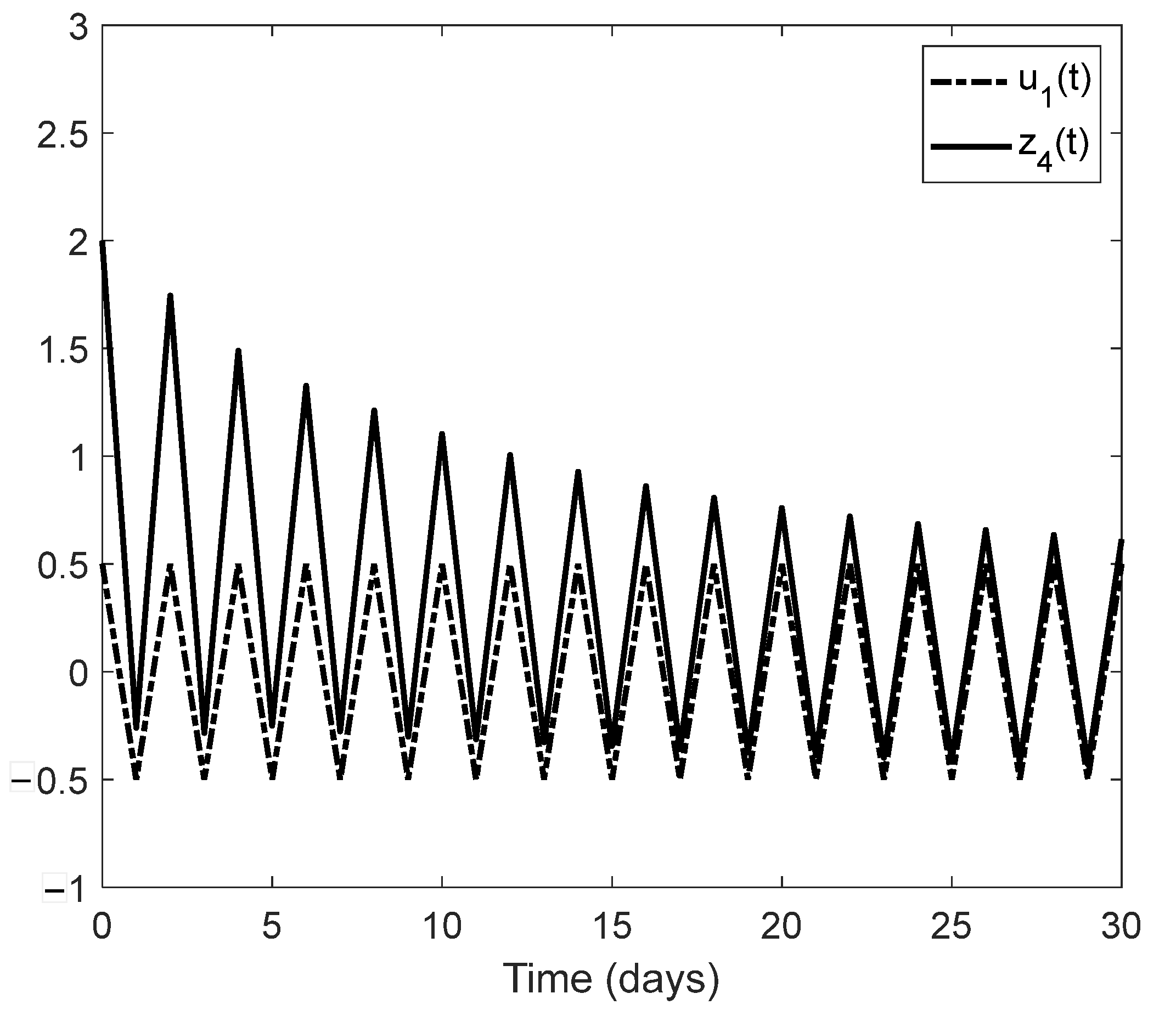
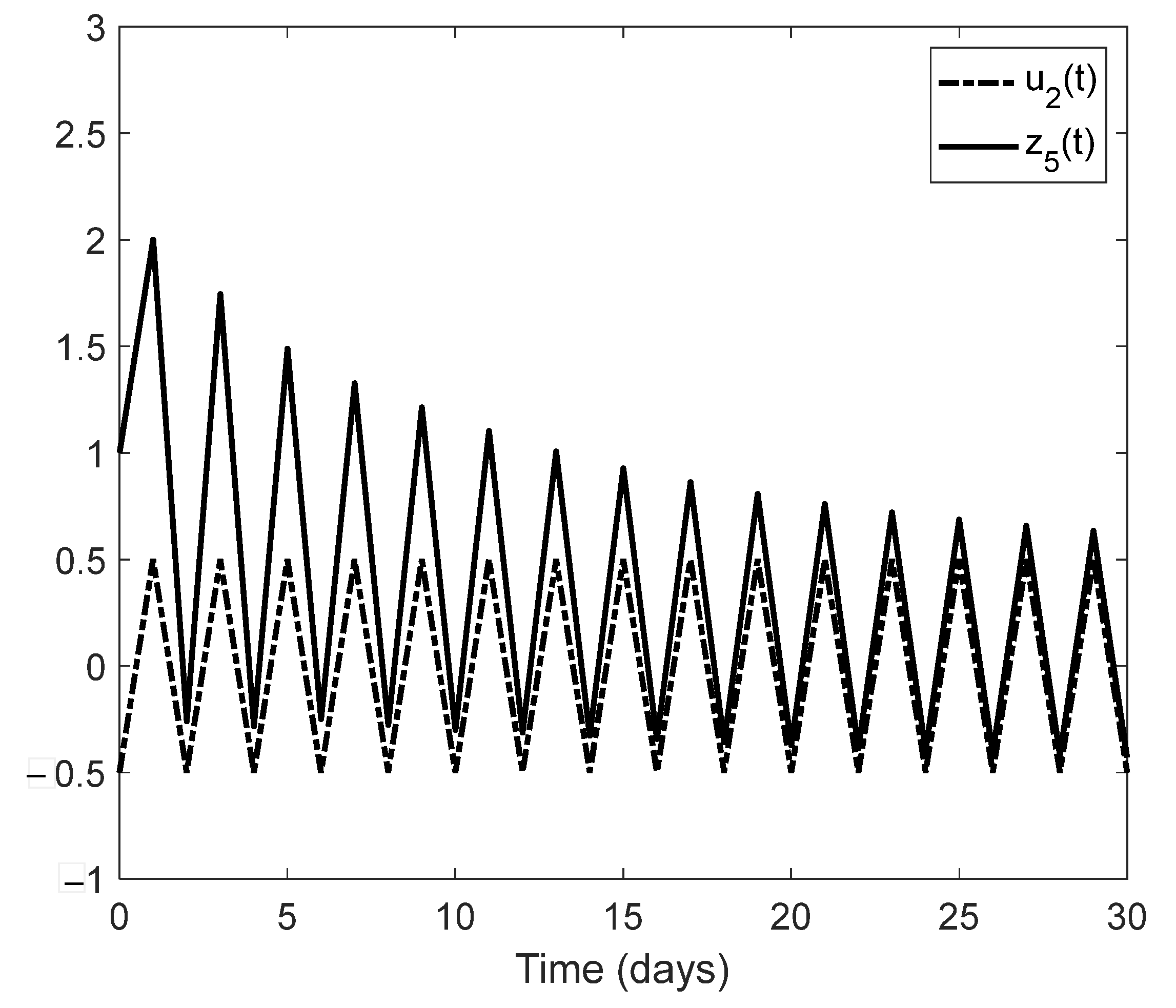
We showed examples of when an unknown change in the environment can be estimated together with the state process of an age-structured population. These examples could be starting points of a new line of research concerning a general monitoring system for environmental contamination based on the observation of easily observable age classes of a given indicator species. Another line of research that would go beyond the framework of the present paper might be an extension of the monitoring problem to the case of several interacting, age-structured populations. In this model, we would have to cope with two types of nonlinearity: one leading to the saturation according to the carrying capacity of the environment, and another one describing interspecific interactions such as predation.

Finally, for an outlook, we also mention that, while in the observer design, the system dynamics were known, and from the observation, an unknown state process was estimated. In the case of a structural identification problem, the structure of the system dynamics is known, and we want to recover its unknown parameters. On the structural identifiability of continuous-time nonlinear biological systems, a recent review was written by Villaverde [40]. In the case of discrete-time systems, Anstett et al. [41] may be a useful reference. Since model parameters can be considered as constant state variables, the structural identification problem can be considered as a particular case of the observation problem. In fact, in Section 5 of the present paper, observer design methodology was used to numerically estimate certain changes in population parameters due to abiotic environmental effects. This can be considered a particular case of structural identification. The generalization of this approach to different ecological situations, including several interacting species, could open a new line of research.

References

1. Kalman, R.E.; Falb, P.L.; Arbib, M.A. Topics in Mathematical System Theory; McGraw-Hill: New York, NY, USA, 1969. [Google Scholar]
2. Varga, Z. On observability of Fisher’s model of selection. Pure Math. Appl. 1992, 3, 15–25. [Google Scholar]
3. Gámez, M.; López, I.; Rodríguez, C.; Varga, Z.; Garay, J. Observation and control in models of population genetics. J. Frankl. Inst. 2017, 354, 7359–7384. [Google Scholar] [CrossRef]
4. Sundarapandian, V. Local observer design for nonlinear systems. Math. Comput. Model. 2002, 35, 25–36. [Google Scholar] [CrossRef]
5. Gámez, M.; López, I.; Garay, J.; Varga, Z. Observation and control in a model of a cell population affected by radiation. Biosystems 2009, 96, 172–177. [Google Scholar] [CrossRef] [PubMed] [Green Version]
6. Gámez, M.; López, I.; Varga, Z.; Garay, J. Stock estimation, environmental monitoring and equilibrium control of a fish population with reserve area. Rev. Fish Biol. Fish. 2012, 22, 751–766. [Google Scholar] [CrossRef]
7. López, I.; Gámez, M.; Garay, J.; Varga, Z. Monitoring in a Lotka—Volterra model. Biosystems 2007, 87, 68–74. [Google Scholar] [CrossRef] [Green Version]
8. Varga, Z. Applications of mathematical systems theory in population biology. Period. Math. Hung. 2008, 56, 157–168. [Google Scholar] [CrossRef]
9. Gámez, M. Observation and control in density- and frequency-dependent population models. In Ecological Modeling; Zhang, W.J., Ed.; Nova Science Publishers: New York, NY, USA, 2011; pp. 285–306. [Google Scholar]
10. Varga, Z.; Gámez, M.; López, I. Recent developments in monitoring of complex population systems. Am. J. Oper. Res. 2013, 3, 167–180. [Google Scholar] [CrossRef] [Green Version]
11. López, I.; Puertas, M.L.; Rodríguez, C.; Gámez, M.; Varga, M. Robust observer design by sign-stability for the monitoring of population systems. J. Frankl. Inst. 2019, 356, 2240–2257. [Google Scholar] [CrossRef]
12. Gámez, M.; López, I.; Rodríguez, C.; Varga, Z.; Garay, J. Ecological monitoring in a discrete-time prey-predator model. J. Theor. Biol. 2017, 429, 52–60. [Google Scholar] [CrossRef]
13. Sundarapandian, V. Observer design for discrete-time nonlinear systems. Math. Comput. Model. 2002, 35, 37–44. [Google Scholar] [CrossRef]
14. Gődényné Hajdu, G.; Varga, Z. Observer design for a nonlinear multi-stage population dynamics. In Synergy in the Technical Development of Agriculture and Food Industry: 2-nd. International Conference on Agricultural Engineering, Godollo, Hungary, 9–15 October 2011; Szabó, I., Magó, Z., Kurják, Z., Eds.; Szent István University Publishers: Godollo, Hungary, 2011; p. 88. [Google Scholar]
15. Bernadelli, H. Population waves. J. Burma Res. Soc. 1941, 31, 1–18. [Google Scholar]
16. Leslie, P.H. On the use of matrices in certain population mathematics. Biometrika 1945, 33, 183–212. [Google Scholar] [CrossRef] [PubMed]
17. Leslie, P.H. Some further notes on the use of matrices in certain population mathematics. Biometrika 1948, 35, 213–245. [Google Scholar] [CrossRef]
18. Caswell, H. Matrix Population Models; Sinauer Ass. Inc. Publisher: Souderland, MA, USA, 2001. [Google Scholar]
19. Farina, L.; Rinaldi, S. Positive Linear Systems: Theory and Applications; Wiley: Hoboken, NJ, USA, 2000. [Google Scholar]
20. Pianese, A.; Attias, A.; Varga, Z. Dynamic immigration control improving inverse old-age dependency ratio in a pay-as-you-go pension system. Decis. Support Syst. 2014, 64, 109–117. [Google Scholar] [CrossRef]
21. Gantmacher, F.R. Matrix Theory; Chelsea: New York, NY, USA, 1959. [Google Scholar]
22. Varga, Z. On the asymptotic behaviour of a continuous time, age-specific population growth model. Abstr. Bot. 1986, 10, 357–366. [Google Scholar]
23. Beverton, R.J.H.; Holt, S.J. On The Dynamics of Exploited Fish Populations; Chapman & Hall: London, UK, 1957. [Google Scholar]
24. Getz, W.M.; Haight, R.G. Population harvesting. Demographic models of fish, forest, and animal resources. In Monographs in Population Biology; Princeton University Press: Princeton, NJ, USA, 1989; Volume 27. [Google Scholar]
25. Sharma, R.; Porch, C.E.; Babcock, E.A.; Maunder, M.N.; Punt, A.E. Recruitment: Theory, estimation, and application in fishery stock assessment models. Fish. Res. 2019, 217, 1–4. [Google Scholar] [CrossRef]
26. Jensen, A.L. Simple density-dependent matrix model for population projection. Ecol. Model. 1995, 77, 43–48. [Google Scholar] [CrossRef]
27. Liu, L.; Cohen, J.E. Equilibrium and local stability in a logistic matrix model for age-structured populations. J. Math. Biol. 1987, 25, 73–88. [Google Scholar] [CrossRef]
28. Lefkovitch, L. The study of population growth in organisms grouped by stages. Biometrics 1965, 21, 1–18. [Google Scholar] [CrossRef]
29. Logofet, D.O.; Salguero-Gómez, R. Novel challenges and opportunities in the theory and practice of matrix population modelling: An editorial for the special feature “Theory and Practice in Matrix Population Modelling”. Ecol. Model. 2021, 443, 109457. [Google Scholar] [CrossRef]
30. Logofet, D.O.; Ulanova, N.G. From population monitoring to a mathematical model: A new paradigm of population research. Biol. Bull. Rev. 2022, 12, 279–303. [Google Scholar] [CrossRef]
31. Logofet, D.O.; Klochkova, I.N. Mathematics of Lefkovitch model: Reproductive potential and asymptotic cycles. Mat. Model. 2002, 14, 116–126. [Google Scholar]
32. Svirezhev, Y.M.; Logofet, D.O. Stability of Biological Communities (Revised from the 1978 Russian Edition); Mir Publishers: Moscow, Russia, 1983. [Google Scholar]
33. Logofet, D.O. Matrices and Graphs. Stability Problems in Mathematical Ecology; CRC Press: Boca Raton, FL, USA, 1993; Reprinted in 2018. [Google Scholar]
34. Schreiber, M.M. Integrated Pest Management Systems: A Research Approach (No. 985); Agricultural Experiment Station, Purdue University: West Lafayette, IN, USA, 1987. [Google Scholar]
35. Lima, M.C.F.; de Almeida Leandro, M.E.D.; Valero, C.; Coronel, L.C.P.; Bazzo, C.O.G. Automatic detection and monitoring of insect pests—A review. Agriculture 2020, 10, 161. [Google Scholar] [CrossRef]
36. Guiro, A.; Iggidr, A.; Ngom, D. On the stock estimation for a harvested fish population. Bull. Math. Biol. 2012, 74, 116–142. [Google Scholar] [CrossRef]
37. Isidori, A. Non Linear Control Systems; Springer: New York, NY, USA, 1995. [Google Scholar]
38. Ngom, D.; Iggidr, A.; Guiro, A.; Ouahbi, A. An observer for a nonlinear age-structured model of a harvested fish population. Math. Biosci. Eng. 2008, 5, 337–354. [Google Scholar] [PubMed]
39. Garay, J.; Sebestyén, Z.; Varga, Z.; Gámez, M.; Torres, A.; Belda, J.E.; Cabello, T. A new multistage dynamic model for biological control exemplified by the host-parasitoid system Spodoptera exigua-Chelonusoculator. J. Pest Sci. 2015, 88, 343–358. [Google Scholar] [CrossRef]
40. Villaverde, A.F. Observability and structural identifiability of nonlinear biological systems. Complexity 2019, 2019, 8497093. [Google Scholar] [CrossRef] [Green Version]
41. Anstett, F.; Bloch, G.; Millérioux, G.; Denis-Vidal, L. Identifiability of discrete-time nonlinear systems: The local state isomorphism approach. Automatica 2008, 44, 2884–2889. [Google Scholar] [CrossRef] [Green Version]
Figure 1. Strictly decreasing function q with lim λ + 0 q ( λ ) = , lim λ q ( λ ) = 0 and λ 1 M + 1     q ( M + 1 ) 1 .
Mathematics 10 02707 g001
Figure 2. Trajectories tending to the positive equilibrium.
Mathematics 10 02707 g002
Figure 3. Trajectories running away from zero.
Mathematics 10 02707 g003
Figure 4. The solution of the observer system approached the unknown solution of the original system.
Mathematics 10 02707 g004
Figure 5. The solution of observer (14) with initial value z ( 0 ) = 18 15 9   3 T approaches the “unknown” state process with initial value x ( 0 ) u ( 0 ) = 10 16 5   1.5 T . In particular, z4(t) approaches the “unknown” environmental change of the reproduction rate of the third age class.
Mathematics 10 02707 g005
Figure 6. Estimation of the state process, under the effect of an unknown periodic environmental change, using an observer corresponding to the system extended with the exosystem.
Mathematics 10 02707 g006
Figure 7. Estimation of the “unknown” environmental change, using the same observer as in Figure 6.
Mathematics 10 02707 g007aMathematics 10 02707 g007b
Publisher’s Note: MDPI stays neutral with regard to jurisdictional claims in published maps and institutional affiliations.