Simultaneous State and Kinetic Observation of Class-Controllable Bioprocesses

Abstract

Monitoring of bioprocesses is a challenge in designing modern systems for control. In the biotechnology industry, the lack of reliable hardware sensors for key variables related to the metabolism of microorganisms is a topical problem. This predetermines the progress of a scientific field that relies on the development of software sensors for immeasurable variables. In this paper, a new approach for the monitoring of class-controllable bioprocesses that evolve through various physiological states (metabolic regimes) is proposed. At the core of the approach is the potential to present total biomass as a sum of the biomass concentrations obtained during each of the metabolic regimes. Algorithms for estimation of immeasurable variables and their kinetics are here derived and applied using real experimental data. As a case-study, a fed-batch process for phytase production by E. coli is considered. Effectiveness of the method is proven by using two sets of real experiments. One is used to tune the software sensors and the other to verify the approach. The stability analyses are provided, as well. The obtained results and successful verification confirm the adaptive properties of the approach. The considered software sensors will be further built into an interactive system for training specialists/students of biotechnology.

1. Introduction

The optimization of bioprocess production is related to accurate monitoring of all states inherent to particular microorganism cultivation processes. One of the most effective ways of process monitoring is by real-time data analysis derived from sensors, capable of measuring the relevant process parameters [1]. Such observations create the possibility for all stages of microorganism cultivation to be investigated. Moreover, this information can be used in automated and supervised feedback control to maintain favorable conditions for good product quality and quantity [2]. Unfortunately, access to sensors that meet the requirements for on-line process monitoring is limited. A possible solution of the problem is to utilize the information from hardware sensors as inputs to mathematical models that are able to generate the values of critical variables and parameters from the modelled biological phenomena.

Another solution is the combination of hardware sensors with algorithms for on-line estimations of unmeasurable variables and parameters, known as software sensors (SS) [3]. In the last decades, SSs have become established as promising tools for monitoring different bioprocesses [4,5,6,7,8,9,10,11,12,13]. In [7,11] model-based and data-based SSs are reviewed. It should be noted that the choice of SS method for a specific process and in particular biotechnological processes is not an easy task and requires an analysis of the following information: (i) complexity of the specific process; (ii) full/partial knowledge of the system’ dynamics; (iii) available process information—quality and quantity of available off-line and on-line measurements, the types of noises and uncertainties, etc.

Much research in the field of model-based SS is based on an extended Kalman filter, which leads to development of complex nonlinear algorithms. Moreover, in most cases, and despite some good results, there is no guarantee of the convergence and the stability of these algorithms [7,12].

Other approaches for kinetic rates and state estimation are based on adaptive system theory [4,12,14,15,16,17,18,19], high gain approach [20,21,22], sliding mode theory [23,24], interval SS [25], probabilistic observers [26], etc. All of these methods are very dependent, to different degrees, on the process kinetics knowledge.

One class of observers of unmeasured state variables are the asymptotic observers that do not require knowledge of the process kinetics. A potential problem related to asymptotic observers is the dependence of the estimation convergence rate on the operational conditions [4]. The software sensors from this class have the advantage for giving an acceptable solution to one of the main challenges in bioprocess monitoring—the lack of process reproducibility and uncertainty of parameter’s values.

Despite a large multiformity of monitoring methods and processes, only a few examples [27,28,29] concern the implementation of SS to processes that evolve different physiological states (metabolic regimes) and are characterized by multiple specific growth rates. Such processes, for example, include intermediate metabolites (acetate at high-cell density fermentation of E. coli and phytase production by E. coli, ethanol at baker yeast production by S. cerevisiae, gluconic acid at fermentation of A. niger, etc.) that are produced and could be consumed during the cultivation. When the intermediate metabolite is the target product, the last phase (oxidative growth on intermediate product) should be avoided.

The reaction scheme of considered processes could be presented as a set of the following three main reactions (metabolic pathways), which correspond to the process’s physiological states:

• Oxidative growth on the main carbon source (S), with a specific growth rate μ₁:

  $$S\stackrel{\mu 1}{\to }X$$

  (1)
• Fermentative growth on the main carbon source, with a specific growth rate μ₂:

  $$S\stackrel{\mu 2}{\to }X+P_{int}$$

  (2)
• Oxidative growth on the intermediate product (P_int), with a specific growth rate μ₃:

  $$P_{int}\stackrel{\mu 3}{\to }X$$

  (3)

  where $X$ is the biomass concentration.

Each one of the physiological conditions is characterized by a different growth rate of biomass. To track the dynamics of the whole process, it is necessary to propose algorithms for estimation of the growth rates. In [27], Pomerleau and Perrier proposed and experimentally validated an on-line estimation algorithm for multiple reaction rates. This procedure was applied to baker’s yeast fermentation. The algorithm requires the on-line measurement of two or three state variables. In [16], the presented approach for on-line monitoring of three biomass growth rates and biomass concentration is based on adaptive observer theory, on on-line measurements of dissolved oxygen and carbon dioxide concentrations, as well as on laboratory measurements of biomass concentration. In spite of the adaptive properties of the proposed SS, which estimates the biomass growth rates as unknown time-varying parameters, the resulting large number of tuning parameters does not favor user-friendly synthesis of the estimation scheme. In [14], the relationships between tuning, stability, and dynamics of convergence in observer-based kinetics estimators for stirred-tank bioreactors, proposed in [4], is characterized in detail, both for continuous and for discrete time formulations of the estimation algorithms. The results are illustrated with an application to a baker’s yeast cultivation process, characterized by the physiological states mentioned above.

On the basis of the reaction scheme (1)–(3), physiological states could be described by combinations of sub-models, presenting the process dynamics. One challenge is finding reliable information for switching from one metabolic state to another and switching the sub-models.

In [18], the oxidative capacity presented by a model with constant parameters is proposed as a key parameter (marker) for switching the sub models. In a result, inaccuracies in the estimation are observed, since the values are in a close relationship with the type of the strain and the cultivation conditions.

A new marker for recognizing the regimen bottlenecks is the kinetics of intermediate metabolites, proposed in [28]. The process was monitored by a cascade scheme of the SS, which changes its structure depending on the sign of the marker. At the scheme input are the real-time measurements of the main substrate and the intermediate metabolite, and at the output are the immeasurable variables and parameters. The operability of the scheme is tested, and the results are compared with the experimental data of an E. coli fermentation.

All the proposed solutions mentioned above are based on models with constant coefficients obtained by identification based on one set of experimental data. Due to the non-linear and non-stationary nature of the considered processes, as well as the lack of reproducibility of experimental (in case of verification with another dataset), the results are unsatisfactory. This requires the search for solutions that are based on minimal modeling of bioprocesses, i.e., inclusion of the smallest possible number of kinetic parameters and yield coefficients with constant values while preserving model quality.

The aim of this study is to propose an approach for adaptive monitoring of the class of processes described in scheme (1)–(3) and to derive a suitable SS, as well as the conditions for its stability. Unlike the above cases, where the sum of the multiple specific growth rates determines the whole biomass, here the biomass is considered as the sum of the biomasses obtained during the each of the regimes.

As a case study, monitoring of a fed-batch process for phytase production is considered. The main carbon source and the intermediate metabolite are measured on-line. This allows the derivation of adaptive estimates of the specific growth rates, as well as of biomass concentrations associated with them. Effectiveness of the method is proven by using two real experimental datasets. One was used to tune the SS and the other to verify the approach. The discussion includes analysis of the obtained results and direction for future investigations.

2. A General Description of the SS Synthesis Methodology

The object of study is a class of controllable processes that evolve through different physiological states [14,15,16,17,18,28] during cultivation. Each physiological state is characterized by a different growth rate of biomass. In the considered processes, the target product is functionally related to the biomass concentration.

As can be seen from reaction (3), the main source of carbon is depleted and biomass increases at the expense of the intermediate. Its concentration is usually low, leading to insignificant growth of biomass and low productivity of the target product. To avoid such a result, the processes are controlled by feeding with a basic carbon source. Two modes of control could be used—fed-batch or continuous modes of cultivation.

The dynamic model of the process corresponding to scheme (1)–(2), widely used in the literature [14,16,18,28], is presented as follows:

$$\frac{dX}{dt}= \left({\mu }_1+{\mu }_2\right)X-\frac{F}{V}X$$

(4)

$$\frac{dS}{dt}=-\left(k_1{\mu }_1+k_2{\mu }_2\right)X-\frac{F}{V}\left(S-S_{in}\right)$$

(5)

$$\frac{d{P}_{int}}{dt}=k_3{\mu }_{2}X-\frac{F}{V}{P}_{int}$$

(6)

where $k_1$, $k_2$, and $k_3$ are yield coefficients. For fed-batch mode of cultivation, F is the substrate feed rate and V is the reactor volume. In the case of continuous mode of cultivation, D = F/V, where D is the dilution rate.

This model is used as an operational model for monitoring and control purposes.

As mentioned above, the aim is to propose a new monitoring approach involving a minimum number of yield coefficients.

One possible solution is the application of the Z-transformation approach, proposed in [4], which makes it possible to estimate the kinetics of processes without yield coefficients when certain conditions are met (Appendix A.3). Unfortunately, this approach cannot be applied directly to the considered class of processes described by model (4)–(6) as some of the conditions cannot be satisfied.

For this reason, the dynamics of the process must be presented in such a way that the application of the Z-transformation is possible.

The new idea is to present the biomass concentration as a sum of two parts ($X_1+X_2)$. The first one is connected to biomass concentration as related to the oxidative growth on the main carbon source, the second is connected to biomass concentration as related to the fermentative growth on main carbon source. Therefore, the total biomass concentration is:

$$X=X_1+X_2$$

(7)

The reaction scheme for the considered case is rewritten as follows:

• Oxidative growth on the main carbon source, with a specific growth rate ${\mu }_1$:

  $$S\stackrel{\mu 1}{\to }{X}_1$$

  (8)
• Fermentative growth on the main carbon source, with a specific growth rate ${\mu }_2$:

  $$S\stackrel{\mu 2}{\to }{X}_2+P_{int}$$

  (9)

The dynamical model (4)–(6) is presented as follows:

$$\frac{d{X}_1}{dt}={\mu }_1{X}_1-\frac{F}{V}{X}_1$$

(10)

$$\frac{d{X}_2}{dt}={\mu }_2{X}_2-\frac{F}{V}{X}_2$$

(11)

$$\frac{dS}{dt}=-k_1{\mu }_1{X}_1-k_2{\mu }_2{X}_2-\frac{F}{V}\left(S-S_{in}\right)$$

(12)

$$\frac{d{P}_{int}}{dt}=k_3{\mu }_2{X}_2-\frac{F}{V}{P}_{int}$$

(13)

The transport dynamics, main carbon source, and intermediate product are measured on-line.

Applying the Z-transformation method to the presented process model (10)–(13), the vector Z is a linear combination of the vectors ${\mathit{\xi }}_{\mathbf{1}}$ and ${\mathit{\xi }}_{\mathbf{2}}$ of measured (${\mathit{\xi }}_{\mathbf{1}}$) and unmeasured (${\mathit{\xi }}_{\mathbf{2}}$) variables [4] for the considered case, as follows:

$$\mathit{Z} = A_{\mathbf{1}}{\mathit{\xi }}_{\mathbf{1}} + A_{\mathbf{2}}{\mathit{\xi }}_{\mathbf{2}}$$

(14)

where

$$\mathit{Z}=\left[ \begin{array}{c}{Z}_1\\ Z_2\end{array}\right],\hspace{1em}\hspace{1em}{\mathit{\xi }}_{\mathbf{2}}=\left[ \begin{array}{c}{X}_1\\ X_2\end{array}\right],\hspace{1em}\hspace{1em}{\mathit{\xi }}_{\mathbf{1}}=\left[ \begin{array}{c}S\\ P_{int}\end{array}\right],\hspace{1em}{A}_{\mathbf{2}}=\left[\begin{array}{cc}{\mathrm{k}}_1& 0\\ 0& -{\mathrm{k}}_3\end{array}\right],\hspace{1em}{A}_{\mathbf{1}}=\left[\begin{array}{cc}1& 0\\ 0& 1\end{array}\right]$$

Using the Z-transformation (14), the dynamics of the measured variables ${\mathit{\xi }}_{\mathbf{1}}$ can be presented as functions of $\mathit{Z}$ and ${\mathit{\xi }}_{\mathbf{1}}$ as follows:

$$\frac{dS}{dt}= \left(S-Z_1\right){\mu }_1-k_2{\mu }_2{X}_2-\frac{F}{V}\left(S-S_{in}\right)$$

(15)

$$\frac{d{P}_{int}}{dt}= \left(P_{int}-Z_2\right){\mu }_2-\frac{F}{V}{P}_{int}$$

(16)

where the values of $Z_1$ and $Z_2$ are obtained by solving the following dynamic equations of the components of the vector $\mathit{Z}$:

$$\frac{d{Z}_1}{dt}=-\frac{F}{V}{Z}_1+\frac{F}{V}{S}_{in}-k_2{\mu }_2{X}_2$$

(17)

$$\frac{d{Z}_2}{dt}=-\frac{F}{V}{Z}_2$$

(18)

Equations (17) and (18) are obtained by differentiating Equation (14) and substituting the time derivatives of the process variables with the right-hand sides of dynamic Equations (10)–(13).

As can be seen, the dynamic equation of $Z_2$ does not depend on yield coefficients, while that of $Z_1$ includes the term $\left(-k_2{\mu }_2{X}_2\right).$ This leads to a modified representation of the approach from [4] for the class of processes under consideration, which consists of the following:

(1)

Representation of the process model, Equations (4)–(6), for which Z-transformation cannot be applied, in a new form, Equations (10)–(13) that enables a modified application of the Z-transformation method by the model (15)–(18);

(2)

Unlike the original system, Equations (4)–(6), including three yield coefficients, the new system, Equations (15)–(18), includes only one yield coefficient. The two yield coefficients, $k_1$ and $k_3$, are reduced using the Z-transformation. This makes adaptive estimation of the kinetics and immeasurable variable possible, as will be shown below.

The estimation approach of both specific growth rates (${\mu }_1$, ${\mu }_2$) and biomass concentration $X$ is based on the derived system (15)–(18). Two estimators of specific biomass growth rates are derived using on-line measurements of main carbon source $\left(S\right)$ and intermediate product $\left(P_{int}\right)$. The outputs of these estimators are included in the dynamic equations of $X_1$ and $X_2$ to obtain their estimates, as well as the sum $\hat{X}={\hat{X}}_1+{\widehat{X}}_2$.

The software sensor (estimator) of the specific growth rate ${\mu }_2$ using on-line measurements of the intermediate product $P_{int}$ is described by the following system:

$$\frac{d{Z}_2}{dt}=-\frac{F}{V}{Z}_2$$

(19)

$$\frac{d{\widehat{P}}_{int}}{dt}= \left(P_{int}-Z_2\right){\widehat{\mu }}_2-\frac{F}{V}{P}_{int}+{\gamma }_1\left(P_{int}-{\widehat{P}}_{int}\right)$$

(20)

$$\frac{d{\widehat{\mu }}_2}{dt}= {\gamma }_2\left(P_{int}-{\widehat{P}}_{int}\right) \left(P_{int}-Z_2\right)$$

(21)

$$\frac{dV}{dt}=F$$

(22)

where ${\gamma }_1$ and ${\gamma }_2$ are estimator’s tuning parameters ${\widehat{P}}_{int}, {\widehat{\mu }}_2$—the estimates of the intermediate product and specific growth ${\mu }_2$, $Z_2$—auxiliary variable.

The software sensor of the specific growth rate ${\mu }_1$ using on-line measurements of the main carbon source $S$ is described by the following system:

$$\frac{d{Z}_1}{dt}=-\frac{F}{V}{Z}_1+\frac{F}{V}{S}_{in}-k_2{\widehat{\mu }}_2{\widehat{X}}_2$$

(23)

$$\frac{d\widehat{S}}{dt}= \left(S-Z_1\right){\widehat{\mu }}_1-k_2{\widehat{\mu }}_2{\widehat{X}}_2-\frac{F}{V}\left(S-S_{in}\right)+w_1(S-\widehat{S})$$

(24)

$$\frac{d{\widehat{\mu }}_1}{dt}= w_2\left(S-Z_1\right)(S-\widehat{S})$$

(25)

$$\frac{dV}{dt}=F$$

(26)

where $w_1$ and $w_2$ are the estimator’s tuning parameters; $k_2$ is the yield coefficient for fermentative consumption of the main carbon source; $\widehat{S}$, ${\widehat{\mu }}_1$ contains the estimates of the main carbon source and specific growth ${\mu }_1$; $Z_1$ is the auxiliary variable, and ${\widehat{\mu }}_2$ contains the estimates of the specific growth ${\mu }_2$, obtained by estimator (19)–(22).

Estimates of $X_1$ and $X_2$ are obtained based on the specific growth rates’ estimators (19)–(22) and (23)–(26) using the following dynamic equations:

$$\begin{gathered} \frac{d}{dt}\left[ \begin{array}{c}{\widehat{X}}_1\\ {\widehat{X}}_2\end{array}\right]=\left[\begin{array}{cc}{\widehat{\mu }}_1& 0\\ 0& {\widehat{\mu }}_2\end{array}\right]\left[ \begin{array}{c}{\widehat{X}}_1\\ {\widehat{X}}_2\end{array}\right]-\frac{F}{V}\left[ \begin{array}{c}{\widehat{X}}_1\\ {\widehat{X}}_2\end{array}\right] \\ \frac{dV}{dt}=F \end{gathered}$$

(27)

So, the total biomass estimate is as follows:

$$\widehat{X}={\widehat{X}}_1+{\widehat{X}}_2$$

(28)

Below the stability analysis is given.

Stability analysis

Estimator of the specific growth rate${\mu }_2$

The system of the estimation errors is as follows:

$$\frac{d\mathit{x}}{dt}=A\mathit{x}+\mathit{v}$$

(29)

where $\mathit{x}=\left[\begin{array}{c}{\tilde{P}}_{int}\\ {\tilde{\mu }}_2\end{array}\right]$ is the vector of the estimation errors,

$${\tilde{P}}_{int}=P_{int}-{\widehat{P}}_{int}; \hspace{1em} \hspace{1em}\hspace{1em}{\tilde{\mu }}_2={\mu }_2-{\widehat{\mu }}_2;$$

$$A= \left[\begin{array}{cc}-{\gamma }_1& \left(P_{int}-Z_2\right)\\ -{\gamma }_2\left(P_{int}-Z_2\right)& 0\end{array}\right] \hspace{1em} \mathit{v}=\left[\begin{array}{c}0\\ \frac{d{\mu }_2}{dt} \end{array}\right]$$

Suppose that ${\gamma }_1$ and ${\gamma }_2$ are constants with positive values and ${\mu }_2$ is a differentiable function:

$$0\le \frac{d{\mu }_2}{dt}\le M_2$$

Then, according to the adaptive system theory, the error system is stable if the $\left(P_{int}-Z_2\right)$ is persistently existing. The proof of this fact follows from Theorem A2.6 and Theorem A3.2 presented in [4].

Estimator of the specific growth rate${\mu }_1$

The system of the estimation errors is:

$$\frac{d\mathit{x}}{dt}=A\mathit{x}+\mathit{v}$$

(30)

where $\mathit{x}=\left[\begin{array}{c}\tilde{S}\\ {\tilde{\mu }}_1\end{array}\right]$ is the vector of the estimation errors,

$$\begin{array}{c}\tilde{S}=S-\widehat{S}; \hspace{1em}\hspace{1em}\hspace{1em} {\tilde{\mu }}_1={\mu }_1-{\widehat{\mu }}_1; \hspace{1em}\hspace{1em}\hspace{1em} {\epsilon }_2=S_m-S\\ A= \left[\begin{array}{cc}-{\omega }_1& \left(S-Z_1\right)\\ -{\omega }_2\left(S-Z_1\right)& 0\end{array}\right] \mathit{v}=\left[\begin{array}{c}-k_2{\widehat{\mu }}_2{\widehat{X}}_2\\ \frac{d{\mu }_1}{dt}\end{array}\right]\end{array}$$

Suppose that ${\omega }_1$ and ${\omega }_2$ are constants with positive values and ${\mu }_1$ is a differentiable function:

$$0\le \frac{d{\mu }_1}{dt}\le M_1, 0\le k_2{\widehat{\mu }}_2{\widehat{X}}_2\le M_3$$

Then, in similar manner, the error system is stable if the $\left(S-Z_1\right)$ is persistently existing, which follows from Theorem A2.6 and Theorem A3.2 presented in [4].

3. Results and Discussion

3.1. Case Study: Fed-Batch Process of Phytase Production

3.1.1. Experimental Data of Fed-Batch Phytase Production

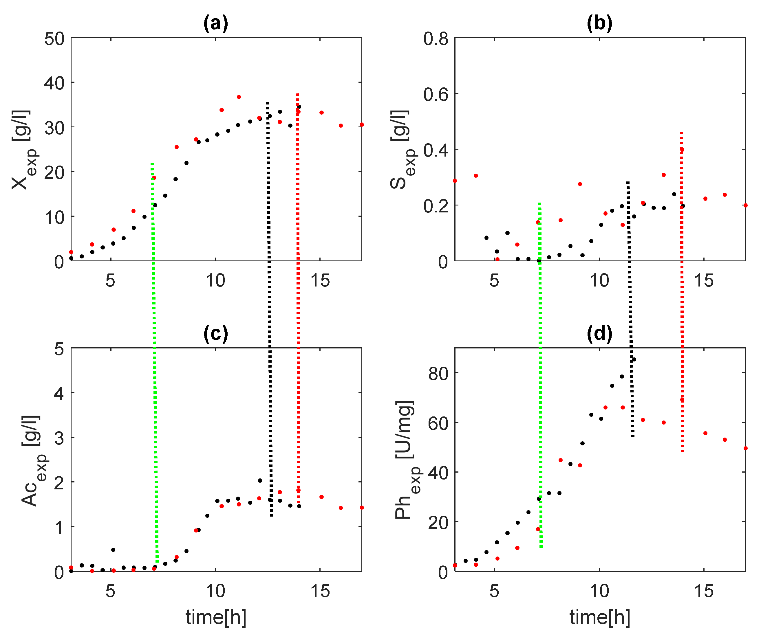
Two experiments of a fed-batch process for phytase production are used here [29,30]. The experimental data are shown in Figure 1 in four subfigures with black (dataset 1) and red (dataset 2) dots. It is noteworthy that in dataset 2, after 11 h, there was a sharp change in metabolism. It is expressed in the cessation in biomass growth (Figure 1a) and production of the target product (Figure 1d). As the feeding continues, substrate concentration increases (Figure 1b). In dataset 1, this effect is not observed. By hour 14 of the cultivation, the biomass increases, as well as the synthesis of the target product, and the substrate stabilizes at a low level. In the processes with the intermediate product of acetate, three metabolic states are observed: oxidative growth of biomass on glucose, oxidative-fermentative growth on glucose, and oxidative growth on glucose and acetate. The transition from the first to the second metabolic state is initiated with the appearance of acetate (Ac) (Figure 1c). As experimental data for the third metabolic state are not available in dataset 2, this gives grounds to consider only the first two metabolic states. For the considered process, it is important that the target product, phytase (Ph), be observed on-line. Its concentration depends on biomass concentration, as will be shown below.

In Figure 1, green dotted lines note the change of the metabolic state from oxidative growth on glucose to oxidative–fermentative growth on glucose for both experiments. Black dotted lines note the change of metabolic state from oxidative–fermentative growth on glucose to oxidative on acetate for the experiment with black dots, and red dotted lines note the change of metabolic state from oxidative–fermentative growth on glucose to oxidative on acetate for the experiment with red dots.

3.1.2. Simulation Results

The approach described by Equations (23)–(28) is applied for estimation of ${\mu }_1$, ${\mu }_2$, $X_1$ and $X_2$ and observation of biomass concentration as a sum of concentrations of $X_1$ and $X_2$ (Equation (28)). The unmeasured variables are biomass ($X$) and target product (Ph). Glucose (S) and acetate (Ac) concentrations are measured on-line.

The simulation investigations are done only for fed-batch mode, i.e., the initial time of simulation is $t_0$ = 4.5 h. The SSs (19)–(22) and (23)–(26) were initially tuned based on dataset 1. The initial values of S and Ac are S($t_0$) = 0.35 g/L and Ac($t_0$) = 0.0476 g/L. The initial value of ${\mu }_1$($t_0$) was calculated using the time-derivative of S from experimental data and Equation (12b), taking into account that at this time, the term F/V is equal to zero and the term ${\widehat{\mu }}_2{\widehat{X}}_2$ accepts negligible value. The calculated value is ${\mu }_1$($t_0$) = 0. 35 1/h. The values of $X_1$($t_0$), $Z_2$($t_0$), ${\mu }_2$($t_0$), and $k_2$ are obtained by optimization together with tuning parameters ${\omega }_1$, ${\omega }_2$, ${\gamma }_1$, and ${\gamma }_2$. The values of ${\omega }_1$ and ${\gamma }_1$ are accepted to be zero and the $X_2$($t_0$) = $X_{exp}$($t_0$) − $X_1$($t_0$). The optimization procedures are based on an evolutionary algorithm [29]. The following criteria is used:

$$J={{\displaystyle \sum }}_{i=1}^n{(X_{exp}\left(i\right)-({\widehat{X}}_1\left(i\right)+{\widehat{X}}_2\left(i\right))}^2+{(S_{exp}\left(i\right)-\widehat{S}\left(i\right))}^2+{(A_{exp}\left(i\right)-\widehat{A}\left(i\right))}^2$$

where n is the number of data points for each process variable (X, S, A); $X_{exp}$, $S_{exp}$, and $A_{exp}$ are the biomass, substrate, and acetate experimental data; ${\widehat{X}}_1, {\widehat{X}}_2, \widehat{S},\widehat{Ac}$ are the biomasses $X_1$, $X_2$, glucose S, and acetate Ac estimates.

The obtained values of tuning parameters are ${\omega }_1=201, {\omega }_2=1, {\gamma }_1=40, {\gamma }_2=5$. The optimized values of $X_1$($t_0$) = 2.7 g/L, $Z_2$($t_0$) = 0.4 1/h, ${\mu }_2$($t_0$) = 0.3 1/h and $k_2$ = 52.3. The value of $X_2$($t_0$) is obtained by $X_2$($t_0$) = $X_{exp}$($t_0$) − $X_1$($t_0$) = 0.1 g/L.

The same values of tuning parameters are applied at verification of the algorithms.

The phytase production depends functionally on biomass growth as follows:

$$\frac{d\widehat{Ph}}{dt}=k_{ph1} {\widehat{\mu }}_1{\widehat{X}}_1+k_{ph2}{\widehat{\mu }}_2{\widehat{X}}_2-\frac{F}{V}Ph$$

(31)

where the values of parameters were obtained by optimization procedure, as follows:

$$k_{ph1} =0.4 \mathrm{and} k_{ph2}=1.7.$$

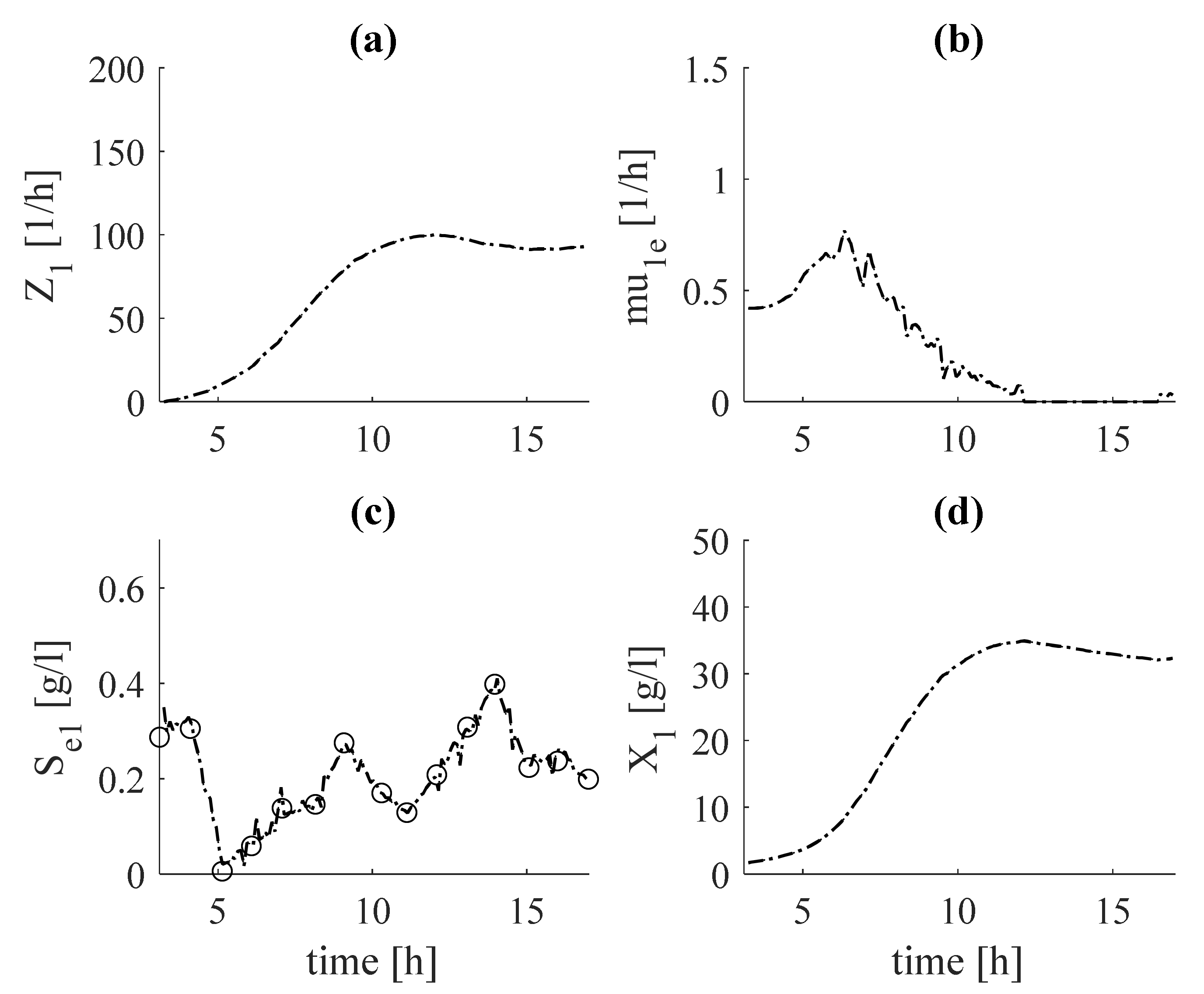
In Figure 2, the results after tuning the ${\mu }_1$ estimator (Equation (25)) based on the substrate S observer (Equation (24)) are shows in subfigures (Figure 2b) and (Figure 2c), respectively. In subfigures (Figure 2a) and (Figure 2d) the estimates of $Z_1$ (Equation (23)) and $X_1$ (Equation (27)), respectively, are shown.

In Figure 3, the verification of the obtained variables and parameters based on dataset 1 is performed using dataset 2 (with the same tuning parameters).

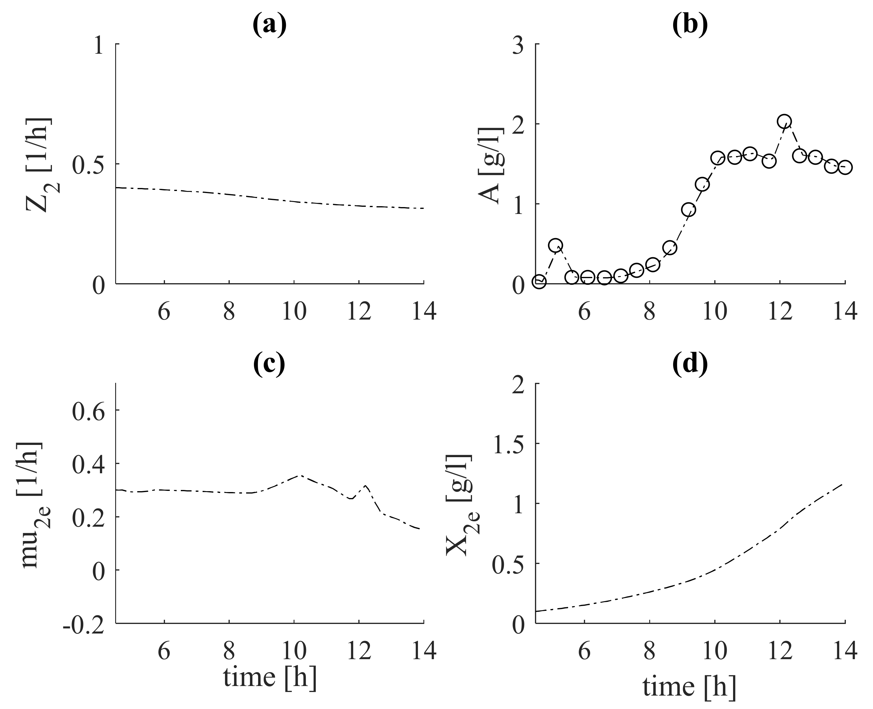
In Figure 4, the results after tuning the ${\mu }_2$ estimator (Equation (21)) based on the intermediate metabolite, Ac, observer (Equation (20)) are shows in subfigures (Figure 4c) and (Figure 4b), respectively. In subfigures (Figure 4a) and (Figure 4d) the estimates of $Z_2$ (Equation (19) and $X_2$ (Equation (27)), are shown, respectively.

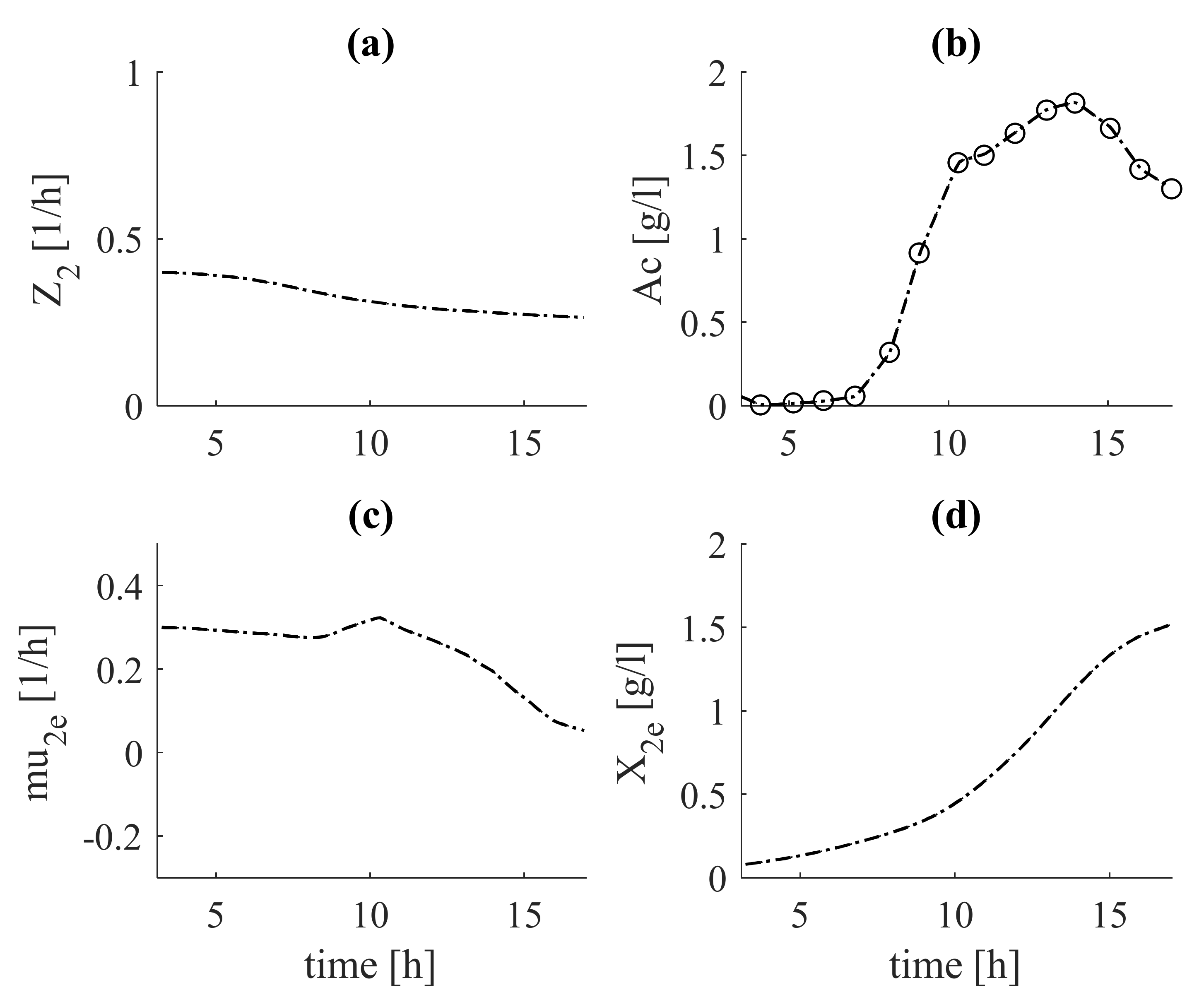
In Figure 5, the verification of the variables and parameters from Figure 4 was performed on the basis of the data from Experiment 2 (red dots) with the same tuning parameters.

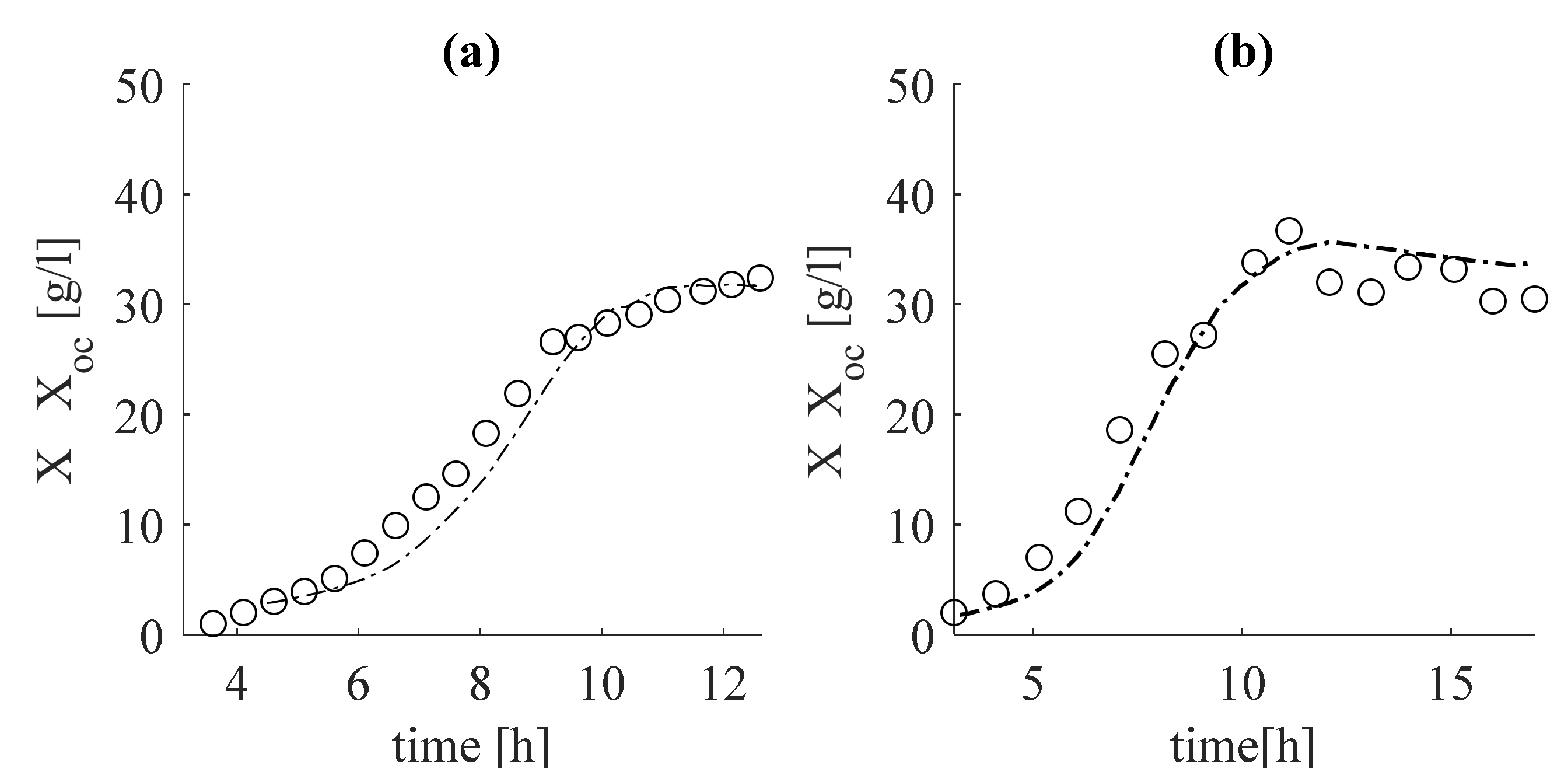
In Figure 6, the estimate of the total biomass, $\widehat{X}$, obtained after summing the estimates ${\widehat{X}}_1 \mathrm{and} {\widehat{X}}_2$ (28), is compared with the data from the experiments in subfigure Figure 6a, with Experiment 1, and subfigure Figure 6b, with Experiment 2.

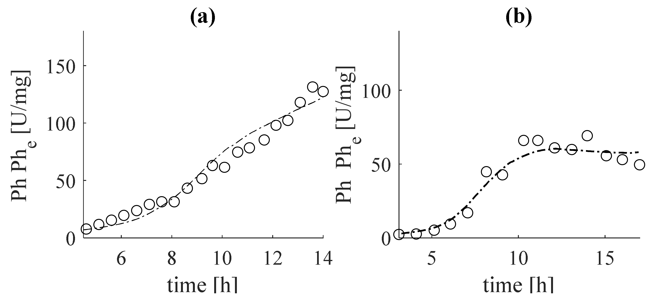
In Figure 7, the estimate of the phytase concentration, $\widehat{Ph}$, obtained by Equation (31) was compared with the data from the experiments in subfigure (Figure 7a) with dataset 1 and in subfigure (Figure 7b) with dataset 2.

The objects of research are bioprocesses, which during cultivation pass through physiological states, presented by dynamic Equation (8). There are different biomass growth rates at each physiological state. This fact gives grounds to present the total biomass as a sum of the biomass concentrations obtained during each of the regimes. During the fermentative growth of biomass, the production of acetate begins. As $X$ and Ac grow on the basis of the main carbon source (glucose) and there is a functional relationship between them, an estimator of ${\mu }_2$ based on measurements of acetate can be derived. Since the kinetics of acetate are unknown, Z-transformation is used. In this way, the estimator of ${\mu }_2$ is presented with the system (Equations (19)–(22)). The estimator of ${\mu }_1$ is derived following the algorithm described above (Equations (23)–(26)), with glucose concentration as the measured variable. The glucose is used as a substrate for both oxidative and fermentative growth of biomass. For this reason, the obtained estimates of ${\mu }_2$ and $X_2$ are included in the structure of the estimator of ${\mu }_1$ system (Equations (23)–(26)). The kinetics of glucose are represented by the first two terms of Equation (24). Here, a yield coefficient $k_2$ is introduced, which describes the consumption of glucose for the fermentative growth of biomass $X_2$. In subfigures (Figure 2c) and (Figure 3c), the estimates of the measured variable (glucose) with the experimental data for both fermentations are compared.

It is noteworthy that the estimates are in complete agreement with the experimental data. This guarantees that the results obtained for ${\mu }_1$, both in the tuning (Figure 2b) and in the verification (Figure 3b) adequately estimate the specific growth rate ${\mu }_1$. The same conclusion can be drawn from the estimator presented by system (19)–(22), based on the measured intermediate metabolite acetate (see Figure 4b and Figure 5b), as well as concerning specific growth rate ${\mu }_2$ (see Figure 4c and Figure 5c). Regarding the estimates of total biomass (Figure 6a) and the target product of phytase (Figure 7a), it can be noted that the estimates of dataset 1 coincide with the real experimental data of these variables. During the verification, some deviations from the measurements are observed, but the tendency is preserved. This may be due to inaccuracies in laboratory measurements of these variables.

To highlight the advantages of the proposed method, the results present here are compared to another method applied to the same set of experimental data [29], where a process model is derived and 26 parameters are identified. The results of the verification in [29] are similar to those obtained by the proposed method whereby only one yield coefficient and four estimator tuning parameters are included in the SS structure.

4. Conclusions

A new method for monitoring of class-controllable bioprocesses characterized by multiple specific growth rates has been proposed. In this method, it is assumed that biomass can be considered as a sum of the biomass concentrations, obtained during different metabolic regimes. This allows each of the components of biomass to be estimated through asymptotic observers on the basis of one of the measured variables. According to the classification [7,11], this approach can be considered as a hybrid method between model-based and data-based software sensors. The model-based part includes the dynamic equation of the measured variables. The data-based part is related to the tuning procedure based on the experimental data. In this way, the number of the kinetics parameters is reduced significantly. There are only three coefficients—one for total biomass observation and two for target product observation. The effectiveness of the method is proven by tuning the estimators from data of one experiment and by verification from data of another experiment at the same tuning parameters. The results obtained are very good, although the two experiments have strongly different dynamics.

Further, the method can be used to predict the dynamics of subsequent experiments, as well as for the synthesis of adaptive control of this class of processes.

References

- Mandenius, C.F. Recent developments in the monitoring, modeling and control of biological production systems. Bioprocess Biosyst. Eng. 2004, 26, 347–351. [Google Scholar] [CrossRef] [PubMed]
- Teixeira, A.P.; Oliveira, R.; Alves, P.; Carrondo, M. Advances in on-line monitoring and control of mammalian cell cultures: Supporting the PAT initiative. Biotechnol. Adv. 2009, 27, 726–732. [Google Scholar] [CrossRef] [PubMed]
- Cheruy, A. Software sensors in bioprocess engineering. J. Biotechnol. 1997, 52, 193–199. [Google Scholar] [CrossRef]
- Bastin, G. On-Line Estimation and Adaptive Control of Bioreactors; Elsevier: Amsterdam, The Netherlands, 2013; Volume 1. [Google Scholar]
- Reyes, S.J.; Durocher, Y.; Pham, P.L.; Henry, O. Modern Sensor Tools and Techniques for Monitoring, Controlling, and Improving Cell Culture Processes. Processes 2022, 10, 189. [Google Scholar] [CrossRef]
- Rincón, A.; Hoyos, F.E.; Restrepo, G.M. Design and Evaluation of a Robust Observer Using Dead-Zone Lyapunov Functions—Application to Reaction Rate Estimation in Bioprocesses. Fermentation 2022, 8, 173. [Google Scholar] [CrossRef]
- Lyubenova, V.; Kostov, G.; Denkova-Kostova, R. Model-based monitoring of biotechnological processes—a review. Processes 2021, 9, 908. [Google Scholar] [CrossRef]
- De Becker, K.; Michiels, K.; Knoors, S.; Waldherr, S. Observer and controller design for a methane bioconversion process. Eur. J. Control 2021, 57, 14–32. [Google Scholar] [CrossRef]
- Mainka, T.; Mahler, N.; Herwig, C.; Pflügl, S. Soft sensor-based monitoring and efficient control strategies of biomass concentration for continuous cultures of Haloferax mediterranei and their application to an industrial production chain. Microorganisms 2019, 7, 648. [Google Scholar] [CrossRef] [Green Version]
- Selişteanu, D.; Petre, E.; Roman, M.; Şendrescu, D. Estimation of kinetic rates in a baker’s yeast fed-batch bioprocess by using non-linear observers. IET Control Theory Appl. 2012, 6, 243–253. [Google Scholar] [CrossRef] [Green Version]
- Zhu, X.; Rehman, K.U.; Wang, B.; Shahzad, M. Modern soft-sensing modeling methods for fermentation processes. Sensors 2020, 20, 1771. [Google Scholar] [CrossRef] [Green Version]
- Dochain, D. Automatic Control of Bioprocesses; John Wiley & Sons: Hoboken, NJ, USA, 2013. [Google Scholar]
- Jiang, Y.; Yin, S.; Dong, J.; Kaynak, O. A review on soft sensors for monitoring, control, and optimization of industrial processes. IEEE Sens. J. 2020, 21, 12868–12881. [Google Scholar] [CrossRef]
- Oliveira, R.; Ferreira, E.C.; Feyo de Azevedo, S. Stability, dynamics of convergence and tuning of observer-based kinetics estimators. J. Process Control 2002, 12, 311–323. [Google Scholar] [CrossRef] [Green Version]
- Lyubenova, V.N.; Ignatova, M.N. On-line estimation of physiological states for monitoring and control of bioprocesses. AIMS Bioeng. 2017, 4, 93–112. [Google Scholar] [CrossRef]
- Lubenova, V.; Rocha, I.; Ferreira, E.C. Estimation of multiple biomass growth rates and biomass concentration in a class of bioprocesses. Bioprocess Biosyst. Eng. 2003, 25, 395–406. [Google Scholar] [CrossRef] [Green Version]
- Perrier, M.; De Azevedo, F.I.G.; Ferreira, E.C.; Dochain, D. Tuning of observer-based estimators: Theory and application to the on-line estimation of kinetic parameters. Control Eng. Pract. 2000, 8, 377–388. [Google Scholar] [CrossRef] [Green Version]
- Rocha, I.C.A.P. Model-Based Strategies for Computer-Aided Operation of Recombinant E. coli Fermentation. Ph. D. Thesis, University of Minho, Braga, Portugal, 2003. [Google Scholar]
- Petre, E.; Selişteanu, D.; Şendrescu, D. Adaptive and robust-adaptive control strategies for anaerobic wastewater treatment bioprocesses. Chem. Eng. J. 2013, 217, 363–378. [Google Scholar] [CrossRef]
- Selisteanu, D.; Petre, E.; Marin, C.; Sendrescu, D. High-Gain Observers for Estimation of Kinetics in a Nonlinear Bioprocess. In Proceedings of the IEEE 2009 ICCAS-SICE, Fukuoka, Japan, 18–21 August 2009; pp. 5236–5241. [Google Scholar]
- Selisteanu, D.; Petre, E. Some on adaptive control of a wastewater biodegradation process. J. Control Eng. Appl. Inform. 2004, 6, 48–56. [Google Scholar]
- Čelikovský, S.; Torres-Munoz, J.A.; Dominguez-Bocanegra, A.R. Adaptive high gain observer extension and its application to bioprocess monitoring. Kybernetika 2018, 54, 155–174. [Google Scholar] [CrossRef] [Green Version]
- Nuñez, S.; Garelli, F.; De Battista, H. Product-based sliding mode observer for biomass and growth rate estimation in Luedeking-Piret like processes. Chem. Eng. Res. Des. 2016, 105, 24–30. [Google Scholar] [CrossRef]
- Battista, H.; Picó, J.; Garelli, F.; Navarro, J.L. Reaction rate reconstruction from biomass concentration measurement in bioreactors using modified second-order sliding mode algorithms. Bioproc. Biosyst. Eng. 2012, 35, 1615–1625. [Google Scholar] [CrossRef]
- Petre, E.; Selişteanu, D.; Roman, M. Nonlinear robust adaptive control strategies for a lactic fermentation process. J. Chem. Technol. Biotechnol. 2018, 93, 518–526. [Google Scholar] [CrossRef]
- Chachuat, B.; Bernard, O. Probabilistic observers for a class of uncertain biological processes. Int. J. Robust Nonlinear Control 2006, 16, 157–171. [Google Scholar] [CrossRef] [Green Version]
- Pomerleau, Y.; Perrier, M. Estimation of multiple specific growth rates in bioprocesses. AIChE J. 1990, 36, 207–215. [Google Scholar] [CrossRef]
- Zlatkova, A.; Lyubenova, V.; Dudin, S.; Ignatova, M. Marker for switching of multiple models describing E. coli cultivation. Comptes Rendus L’académie Bulg. Sci. 2017, 70, 263–273. [Google Scholar]
- Roeva, O.; Pencheva, T.; Tzonkov, S.; Arndt, M.; Hitzmann, B.; Kleist, S.; Miksch, G.; Friehs, K.; Flaschel, E. Multiple model approach to modelling of Escherichia coli fed-batch cultivation extracellular production of bacterial phytase. Electron. J. Biotechnol. 2007, 10, 592–603. [Google Scholar] [CrossRef] [Green Version]
- Kleist, S.; Miksch, G.; Hitzmann, B.; Arndt, M.; Friehs, K.; Flaschel, E. Optimization of the extracellular production of a bacterial phytase with Escherichia coli by using different fed-batch fermentation strategies. Appl. Microbiol. Biotechnol. 2003, 61, 456–462. [Google Scholar] [CrossRef]
Figure 1.
Experimental data; black dots (Experiment 1), red dots (Experiment 2): (a)—biomass concentration, (b)—glucose concentration, (c)—acetate concentration, (d)—phytase concentration.
Figure 2.
Estimation results from tuning of estimator (system (23)–(26)) (with dashed lines, estimates; with circles, experimental data): (a)—auxiliary variable, ; (b)—specific growth rate, ; (c)—substrate concentration, ; (d)—biomass concentration, .
Figure 3.
Verification results from estimator (system (23)–(26)) (with dashed lines, estimates; with circles, experimental data); (a)—auxiliary variable, ; (b)—specific growth rate, ; (c)—substrate concentration, (d)—biomass concentration, .
Figure 4.
Estimation results from tuning of estimator (system (19)–(22)) (with dashed lines, estimates; with circles, experimental data): (a)—auxiliary variable, (b)—acetate concentration, Ac; (c)—specific growth rate, ; (d)—biomass concentration, .
Figure 5.
Verification results from estimator (system (19)–(22)) (with dashed lines, estimates; with circles, experimental data): (a)—auxiliary variable, ; (b)—acetate concentration, Ac; (c)—specific growth rate, ; (d)—biomass concentration, .
Figure 6.
Estimation (a) and verification (b) of full biomass concentration: with dashed lines, estimates; with circles, experimental data.
Figure 7.
Estimation (a) and verification (b) of phytase concentration: with dashed lines, estimates; with circles, experimental data.
Publisher’s Note: MDPI stays neutral with regard to jurisdictional claims in published maps and institutional affiliations. |
© 2022 by the authors. Licensee MDPI, Basel, Switzerland. This article is an open access article distributed under the terms and conditions of the Creative Commons Attribution (CC BY) license (https://creativecommons.org/licenses/by/4.0/).
Share and Cite
MDPI and ACS Style
Lyubenova, V.N.; Ignatova, M.N.; Shopska, V.N.; Kostov, G.A.; Roeva, O.N. Simultaneous State and Kinetic Observation of Class-Controllable Bioprocesses. Mathematics 2022, 10, 2665. https://doi.org/10.3390/math10152665
AMA Style
Lyubenova VN, Ignatova MN, Shopska VN, Kostov GA, Roeva ON. Simultaneous State and Kinetic Observation of Class-Controllable Bioprocesses. Mathematics. 2022; 10(15):2665. https://doi.org/10.3390/math10152665
Chicago/Turabian StyleLyubenova, Velislava Noreva, Maya Naydenova Ignatova, Vesela Nevelinova Shopska, Georgi Atanasov Kostov, and Olympia Nikolaeva Roeva. 2022. "Simultaneous State and Kinetic Observation of Class-Controllable Bioprocesses" Mathematics 10, no. 15: 2665. https://doi.org/10.3390/math10152665
Note that from the first issue of 2016, this journal uses article numbers instead of page numbers. See further details here.