Modified Interaction Method for Response of Group Piles Considering Pile–Soil Slip

Abstract

The existing model for calculating the settlements of group piles is based on the principle of superposition, which fails to calculate the interaction between piles more comprehensively and to take into consideration the influence of slip between pile and soil. In this paper, the interaction between group piles is analyzed from a novel perspective. It is assumed that the interaction between piles is a dynamic equilibrium process, i.e., additional shear forces and additional displacements are continuously transferred between piles until a state of equilibrium is reached. On this basis, we propose a new model for calculating the settlements of group piles considering pile–soil slip. First, a calculation method for pile–side resistance is developed considering the influence of slip. Based on experience with the pile–soil interface, pile–side soils can be categorized as near–pile soil and far–pile soil, and different load–transfer models are applied to describe their mechanical states. By equating pile–side soils into a nonlinear spring and connecting them in series to determine the overall equivalent stiffness considering the effect of pile–soil slip, the pile–side resistance under different loading conditions can be accurately determined. Secondly, equilibrium analysis of the pile unit is carried out when the equilibrium condition is reached, and the stiffness matrix for load transfer is derived. Therefore, in this paper, the interaction between piles is concentrated in this matrix, which makes the proposed model for pile settlement calculation clearer and more concise. Compared with measured data, the proposed method can capture the main features of the load–settlement behavior of group piles.

1. Introduction

Recently, several methods have been proposed in the field of settlement calculation of piles, such as the numerical method, the interaction coefficient method, the shear–displacement method, and the hybrid method. The numerical method has obvious advantages among these methods. By adopting the proper constitutive model, these methods can adequately represent the interaction between piles and soil. The nonlinear characteristic of the pile–side soil can also be represented through these methods [1]. However, these methods have some disadvantages, such as difficulty in establishing the model and determining the parameters. Therefore, many researchers have focused on a simplified calculation method. Poulos and Davis [2] proposed the interaction coefficient method based on elastic theory. The displacement of piles is superimposed on the group piles, and the displacement of pile–side soil is assumed to be unconstrained, which indicates that the reduction and restriction effect of the pile on the displacement of the foundation is ignored. Therefore, the reinforcement–curtain effect of the group piles on the foundation is ignored, and the interaction between piles is amplified, resulting in larger calculation results [3].

Randolph and Worth [4], Ding et al. [5], and Guo and Randolph [6] carried out studies on the shear–displacement method and considered the displacement of soil caused by shear stress as a logarithmic relationship of the radial distance from the pile. The interaction between group piles was calculated by considering the influence of pile–side resistance. Two piles within the calculation range are arbitrarily selected as the research object to establish the calculation method of the interaction between group piles. However, the relative displacement between the pile and soil is not considered in this calculation method, and the equivalent nonlinear stiffness value is a fixed value. The interaction between soil layers cannot be considered, which results in certain limitations.

Based on the above–simplified calculation method, a hybrid method was proposed by O’Neill et al. [7], who adopted the load–transfer method to simulate the settlement of plies under a load. The interaction between different piles was calculated by the shear–displacement method, which effectively integrated the advantages of various simplified calculations. This method was further developed in follow–up research. Chow [2] calculated the response of piles through theoretical load–settlement curves and used the Mindlin method to calculate the interaction between piles and analyze the settlement of group piles in the elastic, homogeneous, isotropic, semi–infinite space. When the nonlinear property of the pile–side resistance is considered, the increment form of the theoretic load–transfer model is employed, in which the shear modulus is replaced by the secant modulus. A hybrid method considering layered soil was proposed by Lee [8], which was modified to simulate the interaction between different types of piles. Clancy and Randolph [3] used a hybrid method to study pile–raft foundations and achieved fairly accurate predictions with respect to settlement. Through the hybrid method, the load–displacement method can be used to simulate the nonlinear settlement of group piles, and the load distribution of the group piles can be reasonably calculated. However, the computation cost increases rapidly with the scale of group piles, and the corresponding simplification and algorithms of large equations need to be improved.

Therefore, a modified method based on the hybrid method is proposed in this paper considering the interaction between piles more completely and predicting the response of group piles in layered soils. Based on the interaction model of pile groups, the pile–side soil is divided into far–pile soil and near–pile soil based on the elastic– and plastic–state pile soil. The hyperbolic load–transfer model and piecewise function model considering softening are used to calculate the equivalent stiffness of the pile–side soil. The nonlinear, two–stage analysis method [9] is adopted by introducing a spring–series system. Compared with the existing methods, the modified method can accurately simulate the slip characteristics of the interface.

The main contribution of this work is consideration of the mutual interaction between piles from a novel perspective. We consider that the piles in the calculation range are affected by each other in a dynamic balancing process. Therefore, the additional shear stress and additional displacement transfer between piles can be derived by force balance analysis until the interaction between pile elements reaches balance. Through the calculation process mentioned above, the load–displacement stiffness matrix and a new force balance calculation method are derived considering the interaction between piles. The interaction between pile–end soil is also considered to accurately calculate the influence of the reinforcement–curtain effect between group piles. The proposed method is validated by the comparison with the load–displacement behavior on site.

2. Nonlinear Load–Transfer Model of Pile–Side Soil

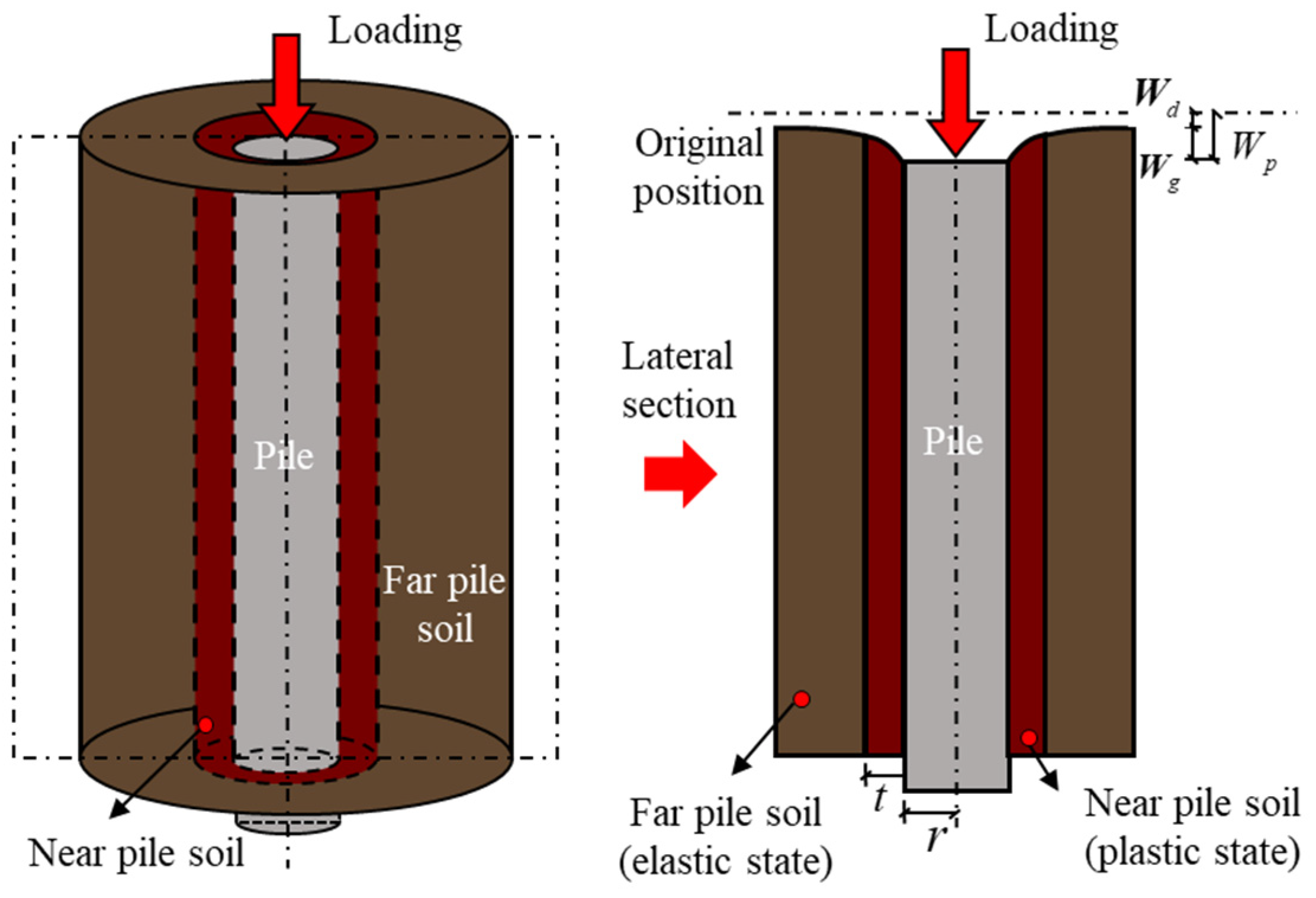
The surface of concrete is rough; therefore, the slip between piles and soil happens in the annular region of the near–pile soil rather than in the close contact regions [10]. In addition, pile–side soils exhibit different mechanical behavior depending on the annular region.

As is shown in Figure 1, when a shear slip occurs, it only happens in the annular region in the near–pile soil, which is regarded as the thickness ($t$) of the shear zone and is generally considered to be five times the average grain size (D50). However, the thickness has no direct effect on shear stress and shear stiffness [11]; therefore, the effect of width is ignored in the calculations presented in this paper, and only the variation of the mechanical properties of the soil in this range is considered. Meanwhile, other parts can be considered to be in an elastic state [12,13], and there is no relative slip between near–pile soil and far–pile soil. Near–pile soil is used to represent the soil in the annular region, which is recorded as $W_g$; and far–pile soil is used to represent the soil in other parts, which is recorded as $W_d$.

It is necessary to consider the effect of the slip between pile and soil and the effect of the elastoplastic state of the pile–side soil on the settlement calculation of group piles. Different load–transfer models are adopted for the soil in different regions, which can reasonably describe the mechanical behavior of different regions.

2.1. Hyperbolic Model for Far–Pile Soil

The classical hyperbolic method was proposed by Wong and Teh [14], in which a hyperbolic relation exists between the shear displacement ($W$) and shear stress ($\tau$) at the interface between pile and soil, as shown in Equation (1):

$$\tau =\frac{W}{\frac{1}{k_s}+R_f\frac{W}{{\tau }_f}}$$

(1)

where $k_s$ is the initial shear stiffness of the interface between pile and soil, ${\tau }_f$ is the initial shear strength, $R_f={\tau }_f/{\tau }_{ult}$ is the failure ratio, and ${\tau }_{ult}$ is the ultimate shear stress on the interface.

For the initial shear stiffness, the empirical formula proposed by Randolph and Worth [4] is employed:

$$k_s^{\prime }=\frac{G_s}{\left[r\ln \left(r_m/r\right)\right]}$$

(2)

where $G_s$ is the shear modulus of the soil, $r$ is the radius of the pile, and $r_m$ is the maximum influence radius of the shear stress. In homogeneous layered soil, the maximum influence radius can be calculated by the following function [15]:

$$r_m=2.5L\frac{{\displaystyle {\displaystyle \sum }_{i=1}^t}{G}_s^i{h}^i}{G_{sm}L}\left(1-\frac{{\displaystyle {\displaystyle \sum }_{i=1}^t}{v}^i{h}^i}{L}\right)$$

(3)

where $t$ is the number of soil layers, $L$ is the pile length, $h^i$ is the thickness of the ith soil layer, $G_s^i$ is the shear modulus of the ith soil layer, $G_{sm}$ is the maximum shear modulus of all layers, and $v^i$ is the Poisson ratio of the ith soil layer.

Frank and Zhao [16] proposed a trifold line based on the pressure meter modulus, which is a more accurate simplified shear displacement model, as shown in the following function. In the proposed initial model, the initial shear stiffness is proportional to the Menard modulus ($E_M$) and inversely proportional to pile radius (r). However, the proposed model does not consider the type of pile and considers only two types of soil, namely cohesive soils and granular soils [17].

$$k_s^{″}=\frac{{\alpha }_s{E}_M}{2r}$$

(4)

where ${\alpha }_s$ is the scale parameter, ${\alpha }_s=2$ for cohesive soils, ${\alpha }_s=0.8$ for granular soils, and $E_M$ is the Menard modulus.

The above research shows that the initial shear stiffness at the pile–soil interface in the conventional hyperbolic model is a constant quantity with depth, which causes the value of the ultimate relative displacement ($W_u$) to increase linearly with depth according to the equation $W_u={\tau }_f/k_s$ [18]. According to SSI experimental results, the relative displacement required to achieve ultimate shear strength in most soils is only 1~4 mm and does not vary with depth [19].

Therefore, in this paper, the initial stiffness determined by the ratio of ultimate shear stress and ultimate relative displacement [18] is used to prevent the relative displacement from increasing with depth.

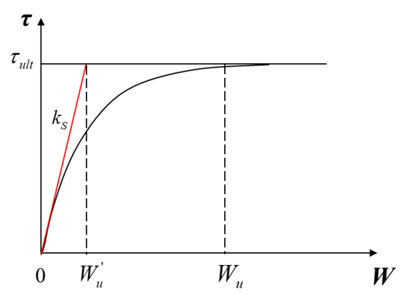
As shown in Figure 2, the pile–side resistance can be calculated as:

$${\tau }_1\left(w\right)=\frac{W}{\frac{1}{{\tau }_f/W_u^{\prime }}+\frac{R_f·W}{{\tau }_f}}=\frac{W}{\frac{1}{{\tau }_f·\chi /W_u}+\frac{R_f·W}{{\tau }_f}}$$

(5)

where $W_u^{\prime }$ is the apparent ultimate relative displacement, i.e., the magnitude of the displacement corresponding to the intersection of the tangent line and the straight line ($\tau ={\tau }_{ult}$) at the origin of the shear displacement curve; $W_u$ is the ultimate relative displacement; and $\chi =W_u/W_u^{\prime }$ is the scale factor, where the values of $\chi$ are larger, the values of ${\tau }_{ult}$ and $\tau \left(W_u\right)$ are closer, and the values of $k_s$ (where $k_s={\tau }_f·\chi /W_u$) are larger. When $\chi =4$, the calculation accuracy can be obtained, avoiding an excessive value of $k_s$ [19].

${\tau }_f$ can be directly measured on site. If there is no corresponding data, the effective stress method [20] can be employed:

$${\tau }_f={\sigma }_h\tan {\phi }^{\prime }+c=K_h{\sigma }_v\tan {\phi }^{\prime }+c$$

(6)

where ${\sigma }_v$ is the effective normal stress of the pile–side soil, ${\phi }^{\prime }$ is the effective friction angle, $K_h$ is the coefficient of lateral pressure of the pile, and $c$ is the effective cohesion intercept.

A study by Yasufuku et al. [21] shows that the pressure of soil on the ground is heavily affected by the construction disturbance and the bearing capacity of the pile foundation. With increased buried depth, the interaction coefficient between piles decreases. The coefficient of the earth pressure for the soil on the ground is assumed as the coefficient of passive earth pressure, and the coefficient of the earth pressure for the pile–end soil is assumed as the coefficient of earth pressure at rest. The definition is as follows:

$$K_h=\left\{1-{\left(\frac{z}{L}\right)}^{\rho }\right\}{K}_p+{\left(\frac{z}{L}\right)}^{\rho }{K}_0$$

(7)

where $z$ is the buried depth of the pile; and $K_0$ and $K_p$ are coefficients of earth pressure at rest and coefficient of passive earth pressure, respectively. The calculation formula is as follows:

$$K_p=\frac{1+\sin {\phi }^{\prime }}{1-\sin {\phi }^{\prime }}$$

(8)

$$K_0=\left(1-\sin {\phi }^{\prime }\right)OC{R}^{\frac{1}{2}}$$

(9)

where OCR is the overconsolidation ratio, and $\rho =0.4{(1-\sin {\phi }^{\prime })}^2$ is the calculation parameter.

2.2. Piecewise Function Model of the Near–Pile Soil

According to observations of shear tests of the pile–soil interface [10], shear displacement of soil around the pile happens with increased shear stress at the pile–soil interface. When the shear stress reaches the ultimate value, interface slip occurs. With increased shear displacement, the effect of pile–side resistance on the shear displacement of soil decreases. In other words, the shear displacement of the near–pile soil comprises slip and plastic deformation of the soil around the pile.

Hu and Pu [10] and Zhang and Zhang [13] proposed a series of constitutive models based on damage theory through structure–soil interface experiments, which can describe the softening phenomenon of soil after reaching the ultimate shear strength. However, compared to the simplified calculation method, these models involve many parameters, which are not easily determined and limit practical engineering applications.

A piecewise function is used to describe the stress state of soil in the shear band, as shown in Figure 3. When the ultimate shear stress is not reached, there is no slip between the pile and soil. The soil is thought to be in an elastic or elastoplastic state, and the resistance of the pile–side soil displacement conforms with the hyperbolic model. When the shear stress reaches the ultimate shear strength, slip occurs between the pile and soil. Under this condition, the soil is in a plastic state. With increased shear displacement, the soil exhibits softening behavior, and shear stress decreases, in accordance with the piecewise function. The equation is as follows:

$${\tau }_2\left(W\right)=\{\begin{array}{ll}\frac{W}{\frac{1}{{\tau }_f·\chi /W_u}+\frac{R_f·W}{{\tau }_f}}\hfill & W\le W_u\hfill \\ R\tau \left(W_u\right)+\tau \left(W_u\right)\left(1-R\right)·T\left(W\right)\hfill & W>W_u\hfill \end{array}$$

(10)

where

$$T\left(W\right)=\mathrm{sech}\left[B\left(W-W_u\right)\right]$$

(11)

where $R$ is the softening ratio, which is the ratio of ultimate resistance of the pile side (${\tau }_{ult}$) to the residual value (${\tau }_{ur}$); and $R$ = 0.85~1.0. $B$ is the control parameter, which indicates the speed of the softening caused by the slip between the pile and soil after reaching the ultimate shear strength, which normally takes $B$ = 100~300 [22]. The higher the soil strength, the larger value of the $B$.

2.3. Load–Transfer Model of Pile–End Soil

According to experimental observations of piles by Zhang et al. [23] the relation between ${\tau }_b/{\tau }_{bu}$ and $W_b/W_{bu}$ can be fitted well in the form of a hyperbolic curve. Therefore, the resistance of the pile–end soil can be described by the hyperbolic function as follows:

$${\tau }_b=\frac{W_b}{A_b+B_b{W}_b}$$

(12)

where $A$, $B$ are empirical coefficients, $W_b$ is the displacement of the pile–end soil, $W_{bu}$ is the ultimate displacement of the pile–end soil, and ${\tau }_b$ is the resistance of pile–end soil.

According to the recommendation of Randolph and Worth [4], $A$ can be calculated as follows:

$$A_b=\frac{\pi r\left(1-v_b\right)}{4G_b}$$

(13)

where $G_b$ is the shear modulus of the pile–end soil, and $v_b$ is the Poisson ratio of the pile–end soil.

$B$ can be calculated as follows [23]:

$$B_b=\frac{1}{{\tau }_{bf}}=\frac{R_{bf}}{{\tau }_{bu}}=\frac{R_{bf}}{c{N}_{\mathrm{c}}+\overline{{\sigma }_{nb}^{\prime }}{N}_q}$$

(14)

where

$$N_c=\left(N_q-1\right)\cot {\phi }_b^{\prime }$$

(15)

$$N_q={\left(\tan {\phi }_b^{\prime }+\sqrt{1+{\tan }^2{\phi }_b^{\prime }}\right)}^2{e}^{2\psi \tan {\phi }_b^{\prime }}$$

(16)

$$\overline{{\sigma }_{nb}^{\prime }}=\frac{1+2K_0}{3}{\sigma }_{vb}^{\prime }$$

(17)

where $R_{bf}={\tau }_{bu}/{\tau }_{bf}$ is the control parameter, ${\phi }_b^{\prime }$ is the effective friction angle of the pile–end soil, $\psi$ is the angle of the failure surface of the pile end and the horizontal direction, and ${\sigma }_{vb}^{\prime }$ is the effective stress of the pile–end soil.

3. Nonlinear Stiffness of Pile–Side Soil Based on the Series–Equivalent Stiffness Calculation Method

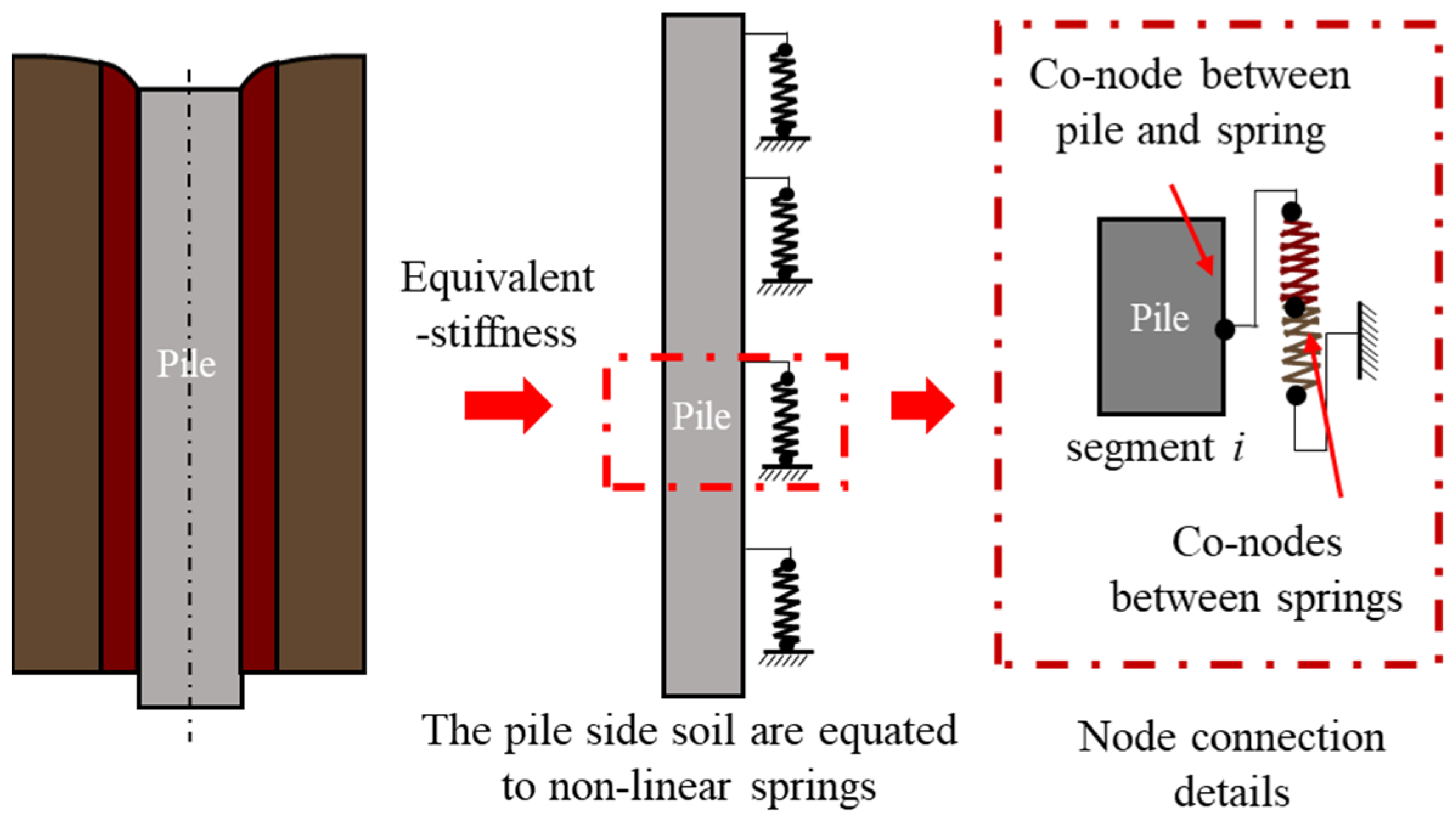
Based on the above load–transfer model, the stiffness of the equivalent nonlinear spring can be determined. Deformation of the soil near the pile side ($W_g$) represents the total displacement, including shear deformation and slip (if slip occurs). The deformation of the soil mass on the far–pile side ($W_d$) indicates the elastic shear deformation of the soil mass on the far–pile side. The settlement displacement of the pile is recorded as $W_p$.

When a slip between pile and soil occurs, the soil in two different regions is connected in series after being equivalent to the nonlinear spring, as shown in Figure 4, and a nonlinear, two–stage analysis method [9] is proposed. Joints between springs are common, and there is no relative slip between the soils of the near– and far–pile sides. Sliding or shear deformation of soil mass on the side of the pile is reflected as deformation of the equivalent nonlinear spring.

The position of the springs connected to the pile segment does not change; therefore, the total displacement of equivalent nonlinear series connected springs that reflect the slip generated on the pile–soil contact surface and the shear deformation of the soil is equal to the displacement of the pile. According to the above boundary conditions, the following equilibrium equations can be listed. Given the boundary condition of the pile segment, the values of $W_g$ and $W_d$ can be obtained by the above binary equation.

$$\{\begin{array}{l}{W}_p=W_g+W_d\\ \tau \left(W_g,z\right)=\tau \left(W_d,z\right)\end{array}$$

(18)

Based on the calculation of secant stiffness of the pile–side soil, the overall equivalent stiffness of the pile–side soil ($k_p$) can be obtained as follows:

$$k_p=\frac{\mathrm{d}\tau \left(z\right)}{\mathrm{d}{w}_z}=\frac{k_g\left(W_g\right)·k_d\left(W_d\right)}{k_g\left(W_g\right)+k_d\left(W_d\right)}$$

(19)

where $k_g$ is the equivalent stiffness of the near–pile soil, $k_d$ is the equivalent stiffness of far–pile soil, and the calculation forms are as follows:

$$k_g\left(W_g\right)={\tau }_2\left(W_u\right)·\left(1-R\right)·T\left(W_g\right)/W_g$$

(20)

$$k_d\left(W_d\right)=\frac{{\tau }_f}{\left(W_u/\chi +R_f·W_d\right)}$$

(21)

4. Group Pile Settlement Calculation Method Based on the Modified Pile–Side Model

According to previous work, the state of the soil on the side of each pile segment can be accurately determined, and its overall equivalent nonlinear stiffness can be calculated. According to the principles of the load–transfer method, force equilibrium analysis of the pile segments can be carried out.

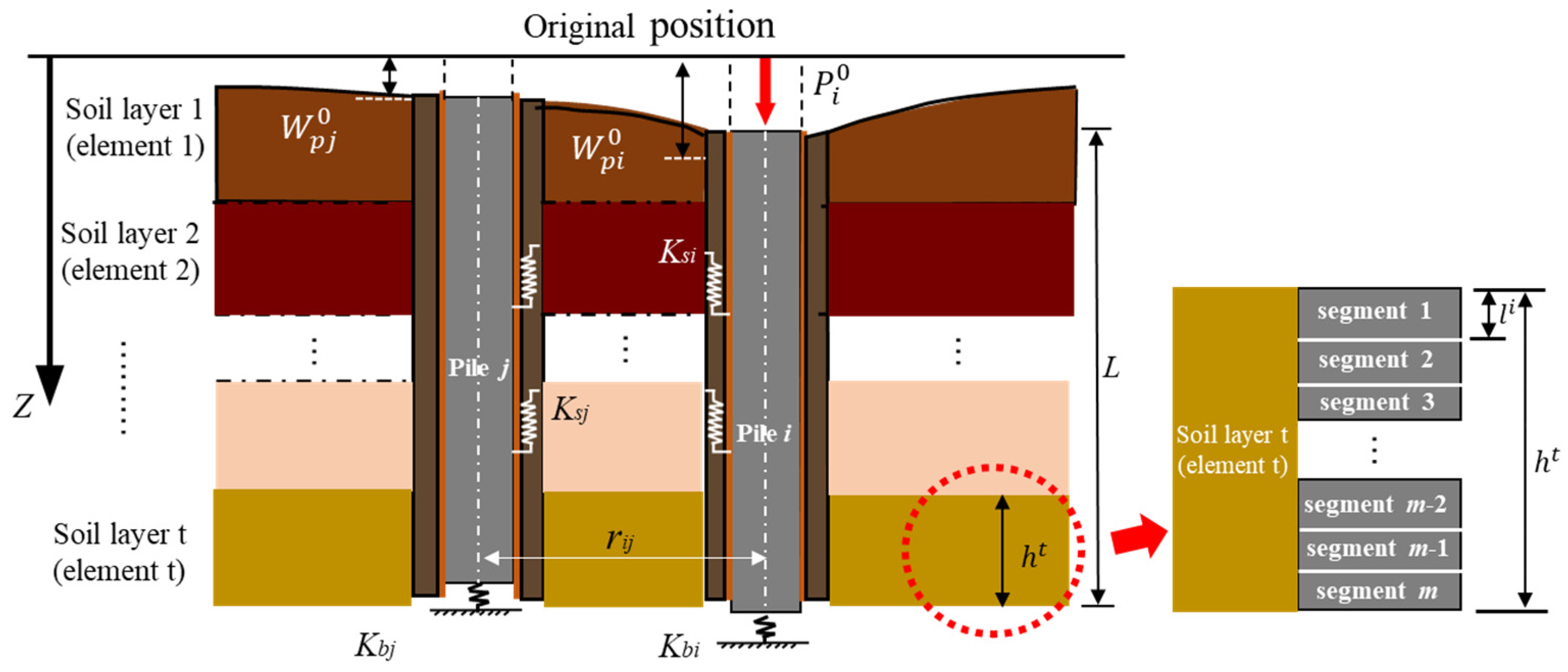
To facilitate the calculation of the interaction between piles, two piles (piles i and j) within the calculation range are arbitrarily selected for research, which are used to establish the interaction model, as shown in Figure 5. Under the action of load, pile i can induce additional shear stress on pile j, and additional shear stress on pile j is generated, which acts on pile i in the same way. The additional stress on pile i can affect pile j until the loop of additional shear stress between the two piles reaches a new balanced state [24].

Based on the calculation methods that consider the linear interaction among unloaded piles and the nonlinear component of the settlement for the loaded piles, the influence of slip of soil mass on the settlement of the pile foundation is considered in this paper through the series–equivalent stiffness method. The elastic and plastic states of the soil mass on the side of the pile are affected not only by the pile head load but by the interaction between the piles. Therefore, stress balance analysis of the pile segment is carried out after the interaction between the two piles reaches equilibrium, and the form of load–transfer stiffness matrix considering the interaction between the piles is deduced for calculation.

4.1. Derivation of Load–Transfer Stiffness Matrix Considering Interaction between Piles

The pile is divided into several elements based on the thickness of the layer, and each element is divided into several segments with the same length ($l^i$). A series of segments can be obtained and numbered through the above method, as shown in Figure 5. Based on analysis of pile segment i, the head loads of pile i and j are $p_i^i,p_j^i$ (the superscript represents the serial number of segments, and the subscript represents the serial number of piles), the head displacements of pile i and j are $W_i^i,W_j^i$, and the side resistances of pile i and j are $f_{pi}^i$, $f_{pj}^i$, respectively. According to the force equilibrium in the vertical direction, the equations of each segment are as follows:

$$\begin{array}{c}{E}_{pi}{A}_{pi}\frac{d^2{W}_{pi}^i}{d{z}^2}-f_{pi}{}^i=0\\ E_{pj}{A}_{pj}\frac{d^2{W}_{pj}^i}{d{z}^2}-f_{pj}{}^i=0\end{array}$$

(22)

where $E_{pi}$ and $E_{pj}$ are the elastic modulus of piles i and j, respectively; $A_{pi}$ and $A_{pj}$ are the cross–sectional area of piles i and j, respectively; and $W_{pi}^i,W_{pj}^i$ are the displacement of the piles under loading considering the interaction between piles.

Based on the original calculation method and considering the interaction between piles in the initial state, the equation of pile head load and displacements of each segment can be obtained as follows:

$$\{\begin{array}{c}{f}_{pi}^i=f_i^i+f_{ij}^i\\ f_{pj}^i=f_j^i+f_{ji}^i\end{array}$$

(23)

$$\{\begin{array}{c}{W}_{pi}^i=W_i^i+W_{ij}^i\\ W_{pj}^i=W_j^i+W_{ji}^i\end{array}$$

(24)

where $f_i^i$($f_j^i$) is segment–side resistance of the single pile (i(j)) under loading, $f_{ij}^i$($f_{ji}^i$) is additional side resistance of pile j(i) considering the reinforcement–curtain effect, and $W_{ij}^i$($W_{ji}^i$) is the effect of pile j(i) under the external load on pile i(j). The direction of additional pile displacement is positive when it is the same as the actual displacement of the pile.

According to the method proposed in this paper, the settlement of the ith segment of pile i(j) can be regarded as the superposition effect of ith segment side–soil slip, shear deformation of pile–side soil, and other effects on the ith segment, and the following displacement equilibrium equation for each segment can be obtained:

$$\{\begin{array}{c}{W}_{pi}^i=\frac{f_{pi}^i}{k_{pi}^i}+\frac{f_{pj}^i}{k_{dj}^i}{\xi }_{ij}^i\\ W_{pj}^i=\frac{f_{pj}^i}{k_{pj}^i}+\frac{f_{pi}^i}{k_{di}^i}{\xi }_{ji}^i\end{array}$$

(25)

Based on the assumption that the far–pile soil can be assumed to be in an elastic state, the transfer coefficient (${\xi }_{ij}$) is expressed as follows [4]:

$${\xi }_{ij}\equiv \frac{U_{\mathrm{s}}\left(r_{ij},z\right)}{U_{\mathrm{s}}\left(r_j,z\right)}=\{\begin{array}{ll}\frac{\ln \left(\frac{r_m}{r_{ij}}\right)}{\ln \left(\frac{r_m}{r_j}\right)}\hfill & r_j\le r_{ij}\le r_m\hfill \\ 0\hfill & r_{ij}>r_m\hfill \end{array}$$

(26)

where $r_{ij}$ is the distance between the axis of piles i and j.

The nonlinear spring stiffness of the pile–side soil is calculated from the actual shear or slip deformation (a and b) of the soil. Then, the joint Equations (18) and (24) can be obtained as the following set of equations:

$$\{\begin{array}{l}{W}_{pi}^i=W_i^i+W_{jd}^i{\xi }_{ij}^i\\ W_{pj}^i=W_j^i+W_{id}^i{\xi }_{ji}^i\\ {\tau }_1\left(W_{id}^i,z\right)={\tau }_2\left(W_i^i,z\right)\\ {\tau }_1\left(W_{jd}^i,z\right)={\tau }_2\left(W_j^i,z\right)\end{array}$$

(27)

When the pile displacements ($W_{pi}^i$ and $W_{pj}^i$) do not reach the ultimate shear displacement, the pile–side soil does not reach the plastic state, and the equivalent stiffness is calculated in the elastic state as a whole; when it reaches the ultimate shear displacement, it can be assumed that the pile–side soil reaches the plastic state, and the equilibrium Equation (27) is solved. If there is no solution for $W_i^i$ and $W_j^i$, then the pile–side soil is still calculated in the elastic state by Equation (14); if not, the equilibrium equation can be solved according to Equations (13) and (14) to obtain the equivalent stiffness of the pile segment. Then, the overall equivalent stiffness of the pile–side soil ($k_{pi}^i$) can be obtained by constituting Equation (19).

Constituting Equations (22) and (25), the differential equation can be obtained as follows:

$$\{\begin{array}{c}{W}_{pi}^i=\frac{1}{{\left({\lambda }_1^i\right)}^2}\frac{d^2{W}_{pi}^i}{d{z}^2}+\frac{1}{{\left({\lambda }_3^i\right)}^2}\frac{d^2{W}_{pj}^i}{d{z}^2}{\xi }_{ij}^i\\ W_{pj}^i=\frac{1}{{\left({\lambda }_2^i\right)}^2}\frac{d^2{W}_{pj}^i}{d{z}^2}+\frac{1}{{\left({\lambda }_4^i\right)}^2}\frac{d^2{W}_{pi}^i}{d{z}^2}{\xi }_{ji}^i\end{array}$$

(28)

where ${\left({\lambda }_1^i\right)}^2=\frac{k_{pi}^i}{E_{pi}^i{A}_{pi}}$, ${\left({\lambda }_2^i\right)}^2=\frac{k_{pj}^i}{E_{pj}^i{A}_{pj}}$, ${\left({\lambda }_3^i\right)}^2=\frac{k_{dj}^i}{E_{pj}^i{A}_{pj}}$, ${\left({\lambda }_4^i\right)}^2=\frac{k_{di}^i}{E_{pi}^i{A}_{pi}}$.

In the case of a steel pipe pile, the elastic modulus ($E_{pi}$) can be used directly for calculation. In the case of a concrete pile, the stress–strain relationship proposed by Hognestad [25] is adopted:

$${\sigma }_c=\{\begin{array}{l}{f}_c\left[2\frac{{\epsilon }_c}{{\epsilon }_0}-{\left(\frac{{\epsilon }_c}{{\epsilon }_0}\right)}^2\right]\left({\epsilon }_c⩽{\epsilon }_0\right)\hfill \\ f_c\left(1-0.15\frac{{\epsilon }_c-{\epsilon }_0}{{\epsilon }_{cu}-{\epsilon }_0}\right)\left({\epsilon }_0<{\epsilon }_c⩽{\epsilon }_{cu}\right)\hfill \end{array}$$

(29)

where $f_c$ is stress at the peak of the stress–strain curve of the concrete; ${\epsilon }_c$ is the strain of the concrete; ${\epsilon }_0$ is the strain when the stress is at the peak, taken as 0.002 [25]; and ${\epsilon }_{cu}$ is the ultimate compressive strain of the concrete.

In practical engineering, concrete piles are not allowed to reach the ultimate compressive strain, and the strain without reaching the ultimate value is considered. The tangent linear elastic modulus of concrete is as follows:

$$E_{pi}=\frac{\mathrm{d}\sigma }{\mathrm{d}\epsilon }=\frac{2{\sigma }_0}{{\epsilon }_0}\sqrt{1-\frac{\sigma }{{\sigma }_0}}$$

(30)

where ${\sigma }_0$ is the peak stress of the concrete, calculated from the compressive strength of the concrete core sample [26]. When experimental results are not available, the ultimate compressive strength of concrete ($f_{cu,k}$) can be employed, and $\sigma$ is the mean stress of the pile.

By solving these differential equations, the expression of settlement of each pile can be obtained as follows:

$$\{\begin{array}{l}{W}_{pi}^i=a_1^i{e}^{m_1^i{z}^i}+a_2^i{e}^{m_2^i{z}^i}+a_3^i{e}^{-m_1^i{z}^i}+a_4^i{e}^{-m_2^i{z}^i}\hfill \\ W_{pj}^i=b_1^i{e}^{m_1^i{z}^i}+b_2^i{e}^{m_2^i{z}^i}+b_3^i{e}^{-m_1^i{z}^i}+b_4^i{e}^{-m_2^i{z}^i}\hfill \end{array}$$

(31)

where $a_1^i$~$a_4^i,b_1^i$~$b_4^i$ are undetermined coefficients, and the expressions of $m_1^i$, $m_2^i$ are as follows:

$$\{\begin{array}{c}{(m_1^i)}^2=\frac{\frac{1}{{\left({\lambda }_1^i\right)}^2}+\frac{1}{{\left({\lambda }_2^i\right)}^2}-\sqrt{{\left(\frac{1}{{\left({\lambda }_1^i\right)}^2}+\frac{1}{{\left({\lambda }_2^i\right)}^2}\right)}^2-4\left(\frac{1}{{\left({\lambda }_1^i\right)}^2·{\left({\lambda }_2^i\right)}^2}-\frac{{\xi }_{ij}^i{\xi }_{ji}^i}{{\left({\lambda }_3^i\right)}^2{\left({\lambda }_4^i\right)}^2}\right)}}{2\left(\frac{1}{{\left({\lambda }_1^i\right)}^2·{\left({\lambda }_2^i\right)}^2}-\frac{{\xi }_{ij}^i{\xi }_{ji}^i}{{\left({\lambda }_3^i\right)}^2{\left({\lambda }_4^i\right)}^2}\right)}\\ \\ {(m_2^i)}^2=\frac{\frac{1}{{\left({\lambda }_1^i\right)}^2}+\frac{1}{{\left({\lambda }_2^i\right)}^2}+\sqrt{{\left(\frac{1}{{\left({\lambda }_1^i\right)}^2}+\frac{1}{{\left({\lambda }_2^i\right)}^2}\right)}^2-4\left(\frac{1}{{\left({\lambda }_1^i\right)}^2·{\left({\lambda }_2^i\right)}^2}-\frac{{\xi }_{ij}^i{\xi }_{ji}^i}{{\left({\lambda }_3^i\right)}^2{\left({\lambda }_4^i\right)}^2}\right)}}{2\left(\frac{1}{{\left({\lambda }_1^i\right)}^2·{\left({\lambda }_2^i\right)}^2}-\frac{{\xi }_{ij}^i{\xi }_{ji}^i}{{\left({\lambda }_3^i\right)}^2{\left({\lambda }_4^i\right)}^2}\right)}\end{array}$$

(32)

When the piles are exactly same, $L_i=L_j=L,E_{pi}=E_{pj}=E_P,A_{pi}=A_{pj}=A_P,{\lambda }_i={\lambda }_j=\lambda ,{\xi }_{ij}={\xi }_{ji}=\xi$; and $m_1^i$, $m_2^i$ can be obtained as follows:

$$\{\begin{array}{c}{(m_1^i)}^2=\frac{{\left({\lambda }^i\right)}^2}{1+{\xi }^i}\\ {(m_2^i)}^2=\frac{{\left({\lambda }^i\right)}^2}{1-{\xi }^i}\end{array}$$

(33)

Constituting boundary condition equations ${\mathit{P}}^{\mathit{i}}=\left[\begin{array}{l}{p}_i^i\hfill \\ p_j^i\hfill \end{array}\right],{\mathit{P}}^{\mathit{i}-{\displaystyle 1}}=\left[\begin{array}{l}{p}_i^{i-1}\hfill \\ p_j^{i-1}\hfill \end{array}\right],{\mathit{W}}_{\mathit{p}}^{\mathit{i}}=\left[\begin{array}{l}{W}_{pi}^i\hfill \\ W_{pj}^i\hfill \end{array}\right],{\mathit{W}}_{\mathit{p}}^{\mathit{i}-{\displaystyle 1}}=\left[\begin{array}{l}{W}_{pi}^{i-1}\hfill \\ W_{pj}^{i-1}\hfill \end{array}\right]$ into Equation (31), and the relationship between the load and displacement at the pile head and the pile–end of the ith segment can be obtained as follows:

$$\left[\begin{array}{l}{\mathit{p}}^{\mathit{i}}\hfill \\ {\mathit{W}}_{\mathit{p}}^{\mathit{i}}\hfill \end{array}\right]=\mathit{T}\left[\begin{array}{l}{\mathit{p}}^{\mathit{i}-{\displaystyle 1}}\hfill \\ {\mathit{W}}_{\mathit{p}}^{\mathit{i}-{\displaystyle 1}}\hfill \end{array}\right]=\left[\begin{array}{ll}{T}_1^i\hfill & T_2^i\hfill \\ T_3^i\hfill & T_4^i\hfill \end{array}\right]\left[\begin{array}{l}{\mathit{p}}^{\mathit{i}-{\displaystyle 1}}\hfill \\ {\mathit{W}}_{\mathit{p}}^{\mathit{i}-{\displaystyle 1}}\hfill \end{array}\right]$$

(34)

The elements of load–displacement stiffness matrix $\mathit{T}$ are as follows:

$$\begin{array}{l}{T}_1^i=\frac{1}{2}·\hfill \\ \left[\begin{array}{ll}cosh\left(m_1^i{l}_i\right)+cosh\left(m_2^i{l}_i\right)\hfill & cosh\left(m_1^i{l}_i\right)-cosh\left(m_2^i{l}_i\right)\hfill \\ cosh\left(m_1^i{l}_i\right)-cosh\left(m_2^i{l}_i\right)\hfill & cosh\left(m_2^i{l}_i\right)-cosh\left(m_1^i{l}_i\right)\hfill \end{array}\right]\hfill \end{array}$$

$$\begin{array}{l}{T}_2^i=\frac{1}{2}{E}_p^i{A}_p^i·\hfill \\ \left[\begin{array}{ll}-m_2^{i}sinh\left(m_2^i{l}_i\right)-m_1^{i}sinh\left(m_1^i{l}_i\right)\hfill & m_2^{i}sinh\left(m_2^i{l}_i\right)-m_1^{i}sinh\left(m_1^i{l}_i\right)\hfill \\ m_2^{i}sinh\left(m_2^i{l}_i\right)-m_1^{i}sinh\left(m_1^i{l}_i\right)\hfill & -m_1^{i}sinh\left(m_1^i{l}_i\right)-m_2^{i}sinh\left(m_2^i{l}_i\right)\hfill \end{array}\right]\hfill \end{array}$$

$$\begin{array}{l}{T}_3^i=\frac{1}{2E_p^i{A}_p^i}·\hfill \\ \left[\begin{array}{ll}-\frac{sinh\left(m_2^i{l}_i\right)}{m_2^i}-\frac{sinh\left(m_1^i{l}_i\right)}{m_1^i}\hfill & \left[\frac{sinh\left(m_2^i{l}_i\right)}{m_2^i}-\frac{sinh\left(m_1^i{l}_i\right)}{m_1^i}\right]\hfill \\ \frac{sinh\left(m_2^i{l}_i\right)}{m_2^i}-\frac{sinh\left(m_1^i{l}_i\right)}{m_1^i}\hfill & -\frac{sinh\left(m_1^i{l}_i\right)}{m_1^i}-\frac{sinh\left(m_2^i{l}_i\right)}{m_2^i}\hfill \end{array}\right]\hfill \end{array}$$

$$\begin{array}{l}{T}_4^i=\frac{1}{2}·\hfill \\ \left[\begin{array}{ll}cosh\left(m_1^i{l}_i\right)+cosh\left(m_2^i{l}_i\right)\hfill & cosh\left(m_1^i{l}_i\right)-cosh\left(m_2^i{l}_i\right)\hfill \\ cosh\left(m_1^i{l}_i\right)-cosh\left(m_2^i{l}_i\right)\hfill & cosh\left(m_2^i{l}_i\right)+cosh\left(m_1^i{l}_i\right)\hfill \end{array}\right]\hfill \end{array}$$

4.2. Settlement Calculation Considering the Interaction between Pile–End Soils

The interaction between pile–end soils is similar to that between piles. The load–displacement stiffness matrix of pile–end soils can be derived based on Equation (12). ${\mathit{p}}_b=\left[\begin{array}{l}{p}_{bi}\hfill \\ p_{bj}\hfill \end{array}\right],{\mathit{W}}_b=\left[\begin{array}{l}{W}_{bi}\hfill \\ W_{bj}\hfill \end{array}\right]$, and the load–displacement relationship between pile–end soils is as follows:

$${\mathit{W}}_b=\left[\begin{array}{ll}\frac{1}{k_{bi}}\hfill & \frac{1}{k_{bj}}{\xi }_{bij}\hfill \\ \frac{1}{k_{bi}}{\xi }_{bij}\hfill & \frac{1}{k_{bj}}\hfill \end{array}\right]{\mathit{p}}_b$$

(35)

where $W_{bi}$ and $W_{bj}$ are pile–end settlements of piles i and j, respectively, under the load considering the interaction; and ${\xi }_{bij}$ is the influence of soil at the end of pile j on the soil at the end of pile i, which can be calculated as follows:

$${\xi }_{ij}\equiv \frac{U_{\mathrm{s}}\left(P_b,z\right)}{U_{\mathrm{s}}\left(r_{ij},z\right)}=\frac{P_b\left(1-v\right)}{4r_{0}G}{\displaystyle /}\frac{P_b\left(1-v\right)}{2\pi rG}=\frac{2}{\pi }·\frac{r_j}{r_{ij}}$$

(36)

where $k_{bi}$ and $k_{bj}$ are the equivalent stiffness of the end soil of piles i and j, respectively. The secant stiffness is adopted and calculated as follows:

$$k_b=\frac{1}{A_b+B_b{W}_b}$$

(37)

When there are n piles in the calculation range, Equation (28) has n items. The differential equations solved by Equation (31) can have 2n solutions and corresponding constant coefficients. The displacement and force of pile–end soil can be obtained through the load–settlement curve of the pile–end soil, which means the boundary condition of the differential equation is determined. Then, the constant coefficients and load–displacement stiffness matrix can be deduced, and the settlement equation of each pile can be obtained through the transformation of pile segments.

4.3. Calculation Process

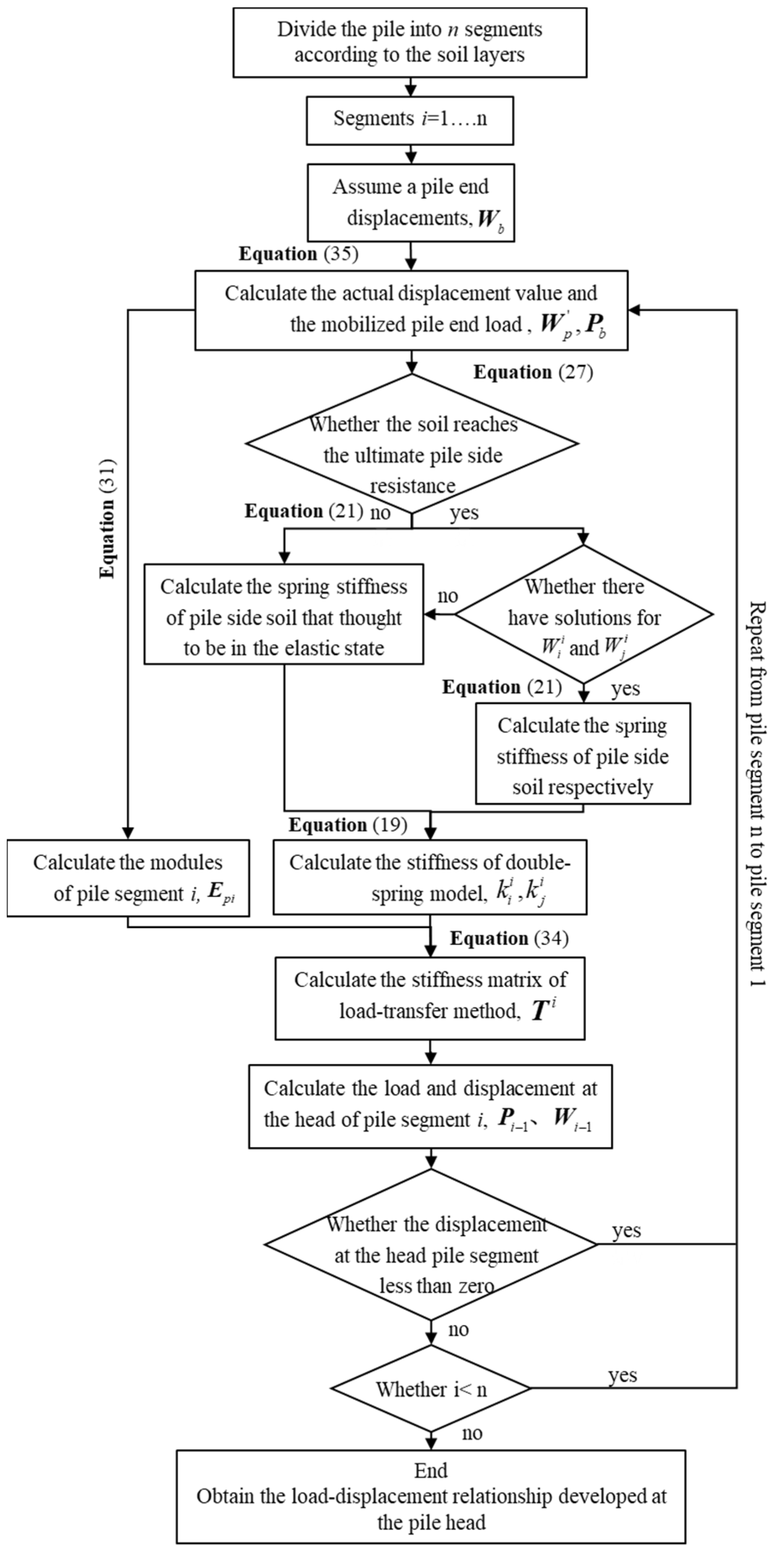
Based on the modified interaction model, the settlement of group piles in the layered foundation can be calculated by the following steps (Figure 6). Under the action of the same pile load, the corresponding pile–end force (${\mathit{p}}_b^i$) can be obtained through Equation (35) based on the assumed pile–end settlement (${\mathit{W}}_b^i$). Then, the elastic modulus of pile segments ($E_p^i$) can be calculated through Equation (30).

Based on the assumed pile–end settlement, the slip state of pile–side soil can also be determined. If it is less than the ultimate relative displacement, the soil on the pile side does not slip, and the soil on the pile side as a whole can be regarded as an elastomer, and Equation (21) is used to calculate the overall equivalent stiffness value. If it is greater than the ultimate relative displacement, the soil on the pile side slips and forms the near and far pile–side soil accordingly; then, the displacement values are substituted into Equation (27) to calculate the displacement values of the near ($W_i^i$) and far pile–side soil ($W_j^i$) and substituted into Equations (20) and (21). Then, the overall nonlinear spring stiffness in series $k_{pi}^i$ and $k_{pj}^i$ can be obtained through Equation (19).

According to the serial connection, the nonlinear spring is equivalent to calculating the stiffness of pile–side soil. The load–displacement stiffness matrix (${\mathit{T}}_i$) can be calculated with Equation (34), and the relations between the segment of pile head force (${\mathit{p}}_{i-1}$) and displacement (${\mathit{W}}_{i-1}$) and between pile–end force (${\mathit{p}}_i$) and displacement (${\mathit{W}}_i$) can be established. Then, the boundary condition of the next loop can be obtained. The load–settlement curve of group piles can be obtained by repeating different calculation values.

5. Validation Results and Discussion

Two cases of the group pile settlement in layered soil are employed to validate the reliability of the modified method.

5.1. Case One

A loading experiment was carried out by Koizumi and Ito [27]. To this end, 3 × 3 equal length piles were used; the layout is shown in Figure 7.

The diameter of the pile is 300 mm, the elastic modulus is 20 GPa, and the buried depth of the pile is 5.5 m. The pile distance is 6 r, which is connected to the pile cap. Double–layered soil exists on the pile side, the upper layer is sandy silt, the depth is 1.7 m, the friction angle is ${23.3}^{\circ }$, the control parameter is $B_1$= 200, and the softening ratio is $R_1$= 0.9. The bottom soil is silty clay, the depth is 3.8 m, and the friction angle is ${21.5}^{\circ }$. The shear strength can be calculated as 30 MPa, the control parameter is $B_2$= 200, and the softening ratio is $R_2$= 0.85, showing that the value of ${\tau }_f$ deduced from the laboratory [2] increases from approximately 25 kPa at the pile head to approximately 40 kPa at the pile tip. The Poisson ratio of the upper soil and bottom layer is 0.5. The failure ratio is $R_f$ = 0.85 and $R_{bf}=$0.85. The parameters $A_b$ and $B_b$ can be calculated with Equations (16) and (17), taken as $1.1\times {10}^{-4}$ and $2.67\times {10}^{-2}$, respectively.

According to the loading experiment, the elastic modulus of the pile–side soil can be calculated based on the proposed equation $E_s=520{\tau }_f$ [2], and the elastic moduli of upper soil and bottom soil are 12.8 MPa and 15.6 MPa, respectively. Then, the load–settlement curve of the pile foundation can be obtained.

As shown in Figure 8, when the load is small, the calculated settlement based on the proposed method is similar to that based on the method proposed by Zhang et al. [28] and Cairo and Conte [2]. The calculated settlement is in agreement with the on–site data, which indicate that there is no relative slip between pile and soil (the soil is in an elastic state). With increased load, the pile–side soil is in an elastoplastic state, and slip between pile and soil occurs. The settlement calculated based on the modified method has large deviations compared with the on–site data, which are not suitable to calculate the settlement of group piles when the pile–side soil is in a plastic state. Compared with other methods, the modified method can determine the mutation point of the load–settlement curve, which can represent the settlement law of the group piles under an external load.

5.2. Case Two

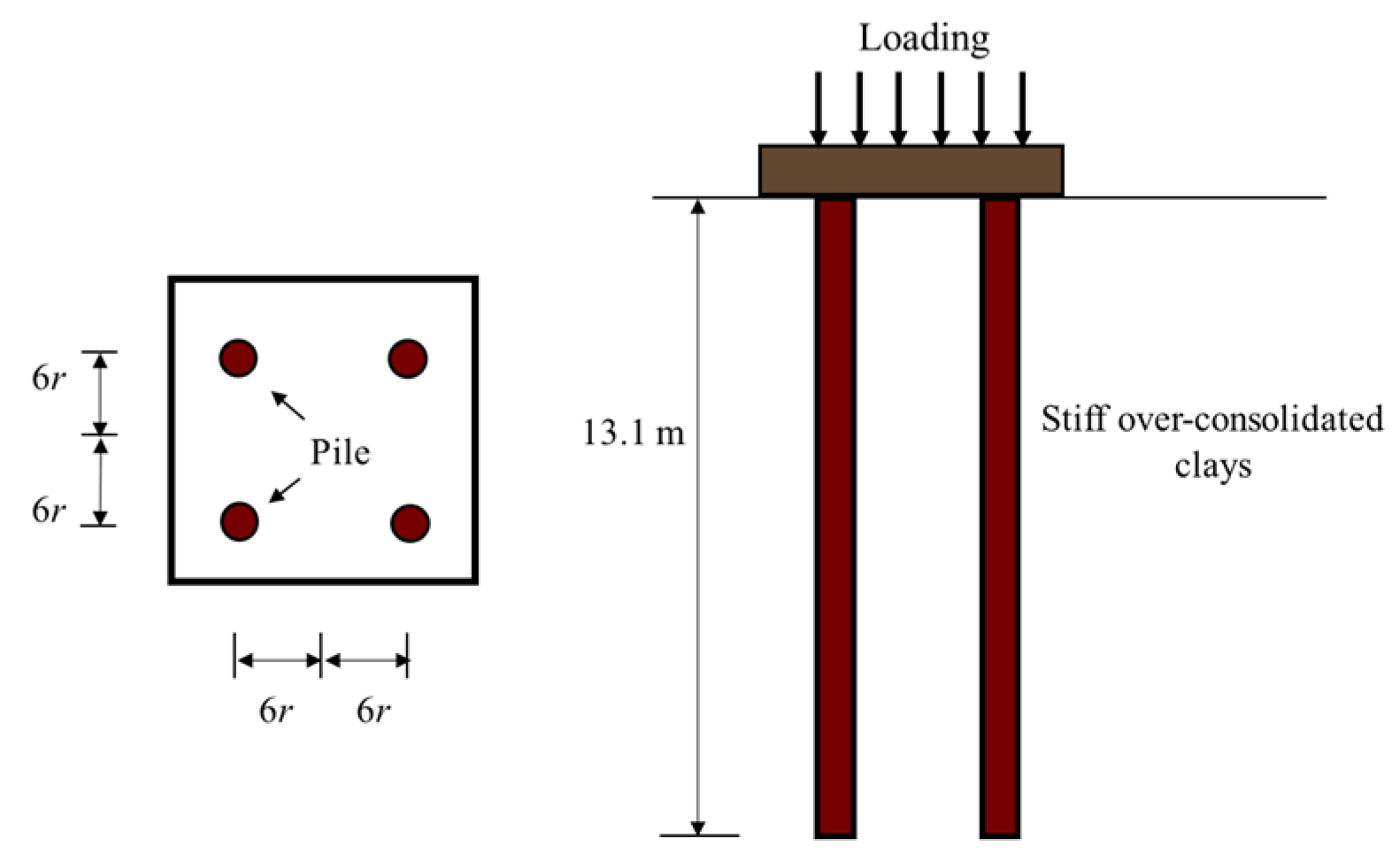
For the model test, a 2 × 2 group–pile axial load test was conducted with a double–layered foundation, as described by Zhang et al. [29]; the layout is shown in Figure 9.

The length of the pile is 13.1 m, and the elastic modulus of the steel pipe pile is 210 GPa. The outer diameter of the steel pipe pile is 137 mm, the thickness of the steel pipe pile is 9.3 mm, and the pile spacing is 6 r. The modulus of the soil is 195 MPa, and the ultimate pile–end resistance is 130 kN. The ultimate pile–side resistance on the ground is 19 kPa, and it increases to 93 kPa linearly in the pile foundation [30]. The softening ratio is R = 0.9, and the Poisson ratio of the soil is 0.3. The failure ratio is $R_f$ = 0.9 and $R_{bf}$ = 0.9, and the control parameter is $B$ = 250. The load–settlement curve of the pile can be calculated as $A_{b }$ = $9.679\times {10}^{-7}$, $B_{b }$ = $4.08\times {10}^{-4}$.

As shown in Figure 10, the calculated results are in agreement with the measured data when the load is small. The pile–side soil is in an elastic state, and there is no relative slip between pile and soil. With increased external load, the pile–side soil is in a plastic state, and slip occurs between pile and soil. The settlement calculated based on the modified method is closer to the measured data than that calculated based on the method proposed by Zhang et al. [29]. The proposed method can accurately represent the mutation point of the load settlement and predicts the settlement law of the pile.

6. Discussion and Conclusions

The modified method for calculating the settlement of group piles was validated in this paper, providing a simplified method for predicting the nonlinear settlement of group piles in layered foundations. According to experimental observations of the interface between pile and soil, slip occurs between pile and soil under shear stress. Based on the hybrid method, the pile–side soil is defined as near–pile soil and far–pile soil depending on whether it is in an elastic or plastic state. The hyperbolic model and the piece–function model considering softening are employed to calculate the equivalent stiffness of the pile–side soil. A spring–series system is adopted to establish a two–stage analysis method.

Combining the advantages of the load–transfer method and the shear–displacement method, the original method with linear superposition of additional displacement and additional shear stress is replaced by the equilibrium equation of pile segment considering the interaction between piles. The interaction between pile–end soil is considered, which can accurately describe the curtain–reinforcement effect. A load–displacement stiffness matrix based on the load–transfer method is derived, and an interaction model between piles is proposed.

The modified method was validated through the load–settlement curves of the field tests. Compared with the traditional interaction model, the modified model is simple and efficient. Furthermore, it can accurately calculate the reinforcement–curtain effect of group piles. The slip between pile and soil is considered to calculate the settlement of group piles more accurately.

The value of the interaction coefficient for the pile–end soil is simplified, which cannot calculate the settlement of group piles accurately; therefore further research is required. The method of determining the value of the interaction coefficient for the pile–end soil deserves further study.

References

- Sheng, D.; Eigenbrod, K.D.; Wriggers, P. Finite element analysis of pile installation using large–slip frictional contact. Comput. Geotech. 2005, 32, 17–26. [Google Scholar] [CrossRef]
- Cairo, R.; Conte, E. Settlement analysis of pile groups in layered soils. Can. Geotech. J. 2006, 43, 788–801. [Google Scholar] [CrossRef]
- Xu, J.; Xu, X.; Yao, W. Improved approach of super–long pile group considering multiple interaction under axial load. Arab. J. Geosci. 2021, 14, 58. [Google Scholar] [CrossRef]
- Randolph, M.F.; Wroth, C.P. An analysis of the vertical deformation of pile groups. Geotechnique 1979, 29, 423–439. [Google Scholar] [CrossRef]
- Ding, X.; Zhang, T.; Li, P.; Cheng, K. A theoretical analysis of the bearing performance of vertically loaded large–diameter pipe pile groups. J. Ocean Univ. China 2016, 15, 57–68. [Google Scholar] [CrossRef]
- Guo, W.D.; Randolph, M.F. An efficient approach for settlement prediction of pile groups. Geotechnique 1999, 49, 161–179. [Google Scholar] [CrossRef]
- O’Neill, M.W.; Hawkins, R.A.; Mahar, L.J. Load transfer mechanisms in piles and pile groups. J. Geotech. Eng. Div. 1982, 108, 1605–1623. [Google Scholar] [CrossRef]
- Lee, C.Y. Settlement of pile groups—Practical approach. J. Geotech. Eng. 1993, 119, 1449–1461. [Google Scholar] [CrossRef]
- Zhang, R.; Zheng, J.; Yu, S. Responses of piles subjected to excavation–induced vertical soil movement considering unloading effect and interfacial slip characteristics. Tunn. Undergr. Space Technol. 2013, 36, 66–79. [Google Scholar] [CrossRef]
- Hu, L.; Pu, J. Testing and modeling of soil–structure interface. J. Geotech. Geoenviron. 2004, 130, 851–860. [Google Scholar] [CrossRef]
- Li, Y.H.; Wang, W.D.; Wu, J.B. Bearing deformation of large–diameter and super–long bored piles based on pile shaft generalized shear model. Chin. J. Geotech. Eng. 2015, 37, 2157–2166. [Google Scholar]
- Poulos, H.G.; Chen, L.T. Pile response due to excavation–induced lateral soil movement. J. Geotech. Geoenviron. 1997, 123, 94–99. [Google Scholar] [CrossRef]
- Zhang, G.; Zhang, J.M. Test study on behavior of interface between structure and coarse grained soil. In Proceedings of the 16th International Conference on Soil Mechanics and Geotechnical Engineering, Osaka, Japan, 12–16 September 2005; IOS Press: Amsterdam, The Netherlands, 2005; pp. 637–640. [Google Scholar]
- Wong, K.S.; Teh, C.I. Negative skin friction on piles in layered soil deposits. J. Geotech. Eng. 1995, 121, 457–465. [Google Scholar] [CrossRef]
- Lee, C.Y. Discrete layer analysis of axially loaded piles and pile groups. Comput. Geotech. 1991, 11, 295–313. [Google Scholar] [CrossRef]
- Frank, R.; Zhao, S.R. Estimation à partir des paramètres pressiométriques de l’enfoncement sous charge axiale de pieux forés dans les sols fins. Bull. Liaison Lab. Ponts Chaussées 1982, 19, 17–24. [Google Scholar]
- Frank, R. Recent developments in the prediction of pile behaviour from pressuremeter results. Symp. Theory Pract. Deep Found. 1985, 1, 69–99. [Google Scholar]
- Alonso, E.E.; Josa, A.; Ledesma, A. Negative skin friction on piles: A simplified analysis and prediction procedure. Geotechnique 1984, 34, 341–357. [Google Scholar] [CrossRef] [Green Version]
- Chen, R.P.; Zhou, W.H.; Cao, W.P.; Chen, Y.M. Improved hyperbolic model of load–transfer for pile–soil interface and its application in study of negative friction of single piles considering time effect. Chin. J. Geotech. Eng. 2007, 29, 824–830. [Google Scholar] [CrossRef]
- Sheil, B.B.; McCabe, B.A. An analytical approach for the prediction of single pile and pile group behaviour in clay. Comput. Geotech. 2016, 75, 145–158. [Google Scholar] [CrossRef]
- Yasufuku, N.; Ochiai, H.; Maeda, Y. Geotechnical analysis of skin friction of cast–in–place piles related to critical state friction angle. Doboku Gakkai Ronbunshu 1999, 617, 89–100. [Google Scholar] [CrossRef]
- Wang, W.D.; Li, Y.H.; Wu, J.B. Pile–soil interface shear model of super long bored pile and its FEM simulation. Rock Soil Mech. 2012, 33, 3818–3824. [Google Scholar] [CrossRef]
- Zhang, Q.Q.; Liu, S.W.; Zhang, S.M.; Zhang, J.; Wang, K. Simplified non–linear approaches for response of a single pile and pile groups considering progressive deformation of pile–soil system. Soils Found. 2016, 56, 473–484. [Google Scholar] [CrossRef]
- Chen, M.Z. Study on Settlement Calculation Theory of Pile Group and Optimal Design of Pile Raft Foundation. Ph.D. Thesis, Zhejiang University, Hangzhou, China, 2000. [Google Scholar]
- Hognestad, E.; Hanson, N.W.; McHenry, D. Concrete stress distribution in ultimate strength design. J. Proc. 1955, 52, 455–480. [Google Scholar]
- Wang, G.; Qiao, S.F.; Wang, G.; Jiang, H.; Singh, J. Cutting depth of pile materials subjected to the abrasive waterjet and its prediction model. Tunn. Undergr. Space Technol. 2022, 124, 104473. [Google Scholar] [CrossRef]
- Koizumi, Y.; Ito, K. Field tests with regard to pile driving and bearing capacity of piled foundations. Soils Found. 1967, 7, 30–53. [Google Scholar] [CrossRef] [Green Version]
- Zhang, Q.Q.; Zhang, Z.M.; He, J.Y. A simplified approach for settlement analysis of single pile and pile groups considering interaction between identical piles in multilayered soils. Comput. Geotech. 2010, 37, 969–976. [Google Scholar] [CrossRef]
- Zhang, Q.Q.; Liu, S.W.; Feng, R.F.; Li, X.M. Analytical method for prediction of progressive deformation mechanism of existing piles due to excavation beneath a pile–supported building. Int. J. Civ. Eng. 2019, 17, 751–763. [Google Scholar] [CrossRef]
- Castelli, F.; Maugeri, M. Simplified nonlinear analysis for settlement prediction of pile groups. J. Geotech. Geoenviron. 2002, 128, 76–84. [Google Scholar] [CrossRef]
Figure 1.
Schematic diagram of the shear deformation and slip between pile and soil.
Figure 2.
Hyperbolic model for the far–pile soil with a modified calculation method of .
Figure 3.
Piecewise function model for the near–pile soil.
Figure 4.
Calculation model of equivalent spring stiffness.
Figure 5.
Interaction model of two piles.
Figure 6.
Computational flow chart for the response of group piles.
Figure 7.
Layout of the pile group and subsoil model.
Figure 8.
Comparison of the predicted and measured load–settlement curve for the group piles [2,27,28].
Figure 9.
Layout of the group piles and subsoil model.
Publisher’s Note: MDPI stays neutral with regard to jurisdictional claims in published maps and institutional affiliations. |
© 2022 by the authors. Licensee MDPI, Basel, Switzerland. This article is an open access article distributed under the terms and conditions of the Creative Commons Attribution (CC BY) license (https://creativecommons.org/licenses/by/4.0/).
Share and Cite
MDPI and ACS Style
Qiao, S.; Dong, C.; Li, G.; Zhou, H.; Wang, G. Modified Interaction Method for Response of Group Piles Considering Pile–Soil Slip. Mathematics 2022, 10, 2616. https://doi.org/10.3390/math10152616
AMA Style
Qiao S, Dong C, Li G, Zhou H, Wang G. Modified Interaction Method for Response of Group Piles Considering Pile–Soil Slip. Mathematics. 2022; 10(15):2616. https://doi.org/10.3390/math10152616
Chicago/Turabian StyleQiao, Shifan, Changrui Dong, Guyang Li, Hao Zhou, and Gang Wang. 2022. "Modified Interaction Method for Response of Group Piles Considering Pile–Soil Slip" Mathematics 10, no. 15: 2616. https://doi.org/10.3390/math10152616
Note that from the first issue of 2016, this journal uses article numbers instead of page numbers. See further details here.