OMPEGAS: Optimized Relativistic Code for Multicore Architecture

Abstract

The paper presents a new hydrodynamical code, OMPEGAS, for the 3D simulation of astrophysical flows on shared memory architectures. It provides a numerical method for solving the three-dimensional equations of the gravitational hydrodynamics based on Godunov’s method for solving the Riemann problem and the piecewise parabolic approximation with a local stencil. It obtains a high order of accuracy and low dissipation of the solution. The code is implemented for multicore processors with vector instructions using the OpenMP technology, Intel SDLT library, and compiler auto-vectorization tools. The model problem of simulating a star explosion was used to study the developed code. The experiments show that the presented code reproduces the behavior of the explosion correctly. Experiments for the model problem with a grid size of $128\times 128\times 128$ were performed on an 16-core Intel Core i9-12900K CPU to study the efficiency and performance of the developed code. By using the autovectorization, we achieved a 3.3-fold increase in speed in comparison with the non-vectorized program on the processor with AVX2 support. By using multithreading with OpenMP, we achieved an increase in speed of 2.6 times on a 16-core processor in comparison with the vectorized single-threaded program. The total increase in speed was up to ninefold.

1. Introduction

Supernovae are the main source of the “elements of life”. In particular, the supernovae are the birthplaces for such elements as carbon, oxygen, and ferrum, which are the basis of all life forms. The great energy output of the supernovae allows them to spread the heavy elements great distances. This contributes to synthesis of complex chemical compounds up to organic ones [1,2].

Together with the various mechanisms of supernova explosions and their material compositions [3,4,5,6,7,8,9,10,11,12,13], it remains important to study the hydrodynamics of supernova explosions. Naturally, because of proportion of the scales between the stars, the supernova remnant, and the core, simulation of such an explosion requires the most powerful supercomputers. Analysis of the top 10 supercomputers in the world shows the prevalence of hybrid architectures, primarily equipped with graphics accelerators and vector processors.

Development of codes for such architectures is a difficult problem. It requires not only application of the appropriate technologies but also a special structure of the numerical method and mathematical models. Several codes adapted for graphics processors (GPU) or the Intel Xeon Phi accelerators have been developed. We review the most interesting solutions.

The WOMBAT code [14] uses a combination of the Message Passing Interface (MPI), Open Multi-Processing (OpenMP), and high-level Single Instruction Multiple Data (SIMD) vectorization technologies. The WOMBAT code is remarkable for its orientation to the target architecture of the supercomputer, which will run it. The code utilizes one-sided MPI communications, which allow one to efficiently implement the exchange of the subdomains overlaps. The specialized Cray MPI is used for optimization of the interprocess communications. The code also uses high-level SIMD vectorization. It appears that the WOMBAT code contains the requirements for modern program implementation of astrophysical codes.The previously developed codes will be used for a long time, but the future is for codes oriented to the specific classes of the supercomputer architectures.

The CHOLLA code [15,16,17] was implemented to conduct numerical experiments using GPUs. It is based on the Corner Transport Upwind method, the essence of which is the propagation of the counterflux scheme in the multidimensional case [18,19]. For storing the computational grid in a GPU, the structure of a mesh containing all the hydrodynamical parameters is used. It is stated that such locality of the data allows one to obtain a more efficient application of the global memory of the graphics processor. Calculation of the time step was performed on graphics processors using the NVIDIA Compute Unified Device Architecture (CUDA) extensions.

The GAMER code [20] solves aerodynamic equations applying the Adaptive Mesh Refinement (AMR) approach to graphics accelerators. For solving aerodynamic equations, the Total Variational Diminishing method is used. For solving the Poisson equation, a combination of the fast Fourier transform method and successive over relaxation is used. The main feature of this software is probably of implementation of the AMR approach on GPUs. Thus, the regular structure of the grid naturally falls onto the GPU architecture, while the tree structure requires a special approach. This approach is based on the application of octets to define the grid. Under this, each octet is projected to a separate thread in the GPU. The main problem is in forming the fake meshes for the octets. Note that solving this problem takes around 63% of the time. However, this procedure can be implemented independently for each octet. The GAMER code was further optimized [21] and extended to solving the magnetic hydrodynamic equations [22].

Approaches such as those described above were implemented in the FARGO3D [23] and the SMAUG [24] codes. The authors of the present work also implemented the GPUPEGAS code [6] for supercomputers with graphics processors and the AstroPhi code for the Intel Xeon Phi in the offload mode [25] and in the native mode using low-level vectorization [26].

The necessity of more efficient utilization of the graphics and vector processors and accelerators will result in creation of new codes. One code is presented in this work. We develop the OMPEGAS code for numerically solving the special relativistic hydrodynamics equations. The numerical algorithm is based on Godunov’s method and the piecewise parabolic method on the local stencil [27,28]. This technique has been successfully applied to a number of astrophysical problems [29,30]. Its main advantages are a high order of accuracy and high efficiency of calculations. The code was developed for shared memory multicore systems with vectorization capabilities. This make it possible to perform experiments on a wide range of computers, from laptops to nodes of cluster supercomputers. Additionally, in future, a hybrid implementation is possible for massive parallel systems.

In Section 2, we provide the hydrodynamical model of the astrophysical flows and describe the numerical method for solving the hydrodynamical equations. Section 3 is devoted to detailing the architecture of the OMPEGAS code and to the study of its performance. Naturally, the code development raised several issues for discussion, which are considered in Section 4. Section 5 is devoted to the numerical experiments. Section 6 concludes the paper.

2. Numerical Model

To describe the gas dynamics, we use the numerical model presented in work [31]. The physical (primitive) variables are: the density $\rho$, vector of velocity $\overrightarrow{v}$, and pressure p. When describing the evolution of gas in the model of special relativistic hydrodynamics, we introduce the concept of special enthalpy h, which is determined by the formula

$$h=1+\frac{\gamma }{\gamma -1}\frac{p}{\rho },$$

(1)

where $\gamma$ is the adiabatic exponent. The relativistic speed of sound $c_s$ is determined by the formula

$$c_s^2=\gamma \frac{p}{\rho h}.$$

(2)

Let us choose the speed of light to be $c\equiv 1$ as the dimensionless unit speed. In this case, the Lorentz factor $\Gamma$ will be determined by the formula

$$\Gamma =\frac{1}{\sqrt{1-{\left(v/c\right)}^2}}=\frac{1}{\sqrt{1-v^2}}.$$

(3)

Thus, the speed module is limited to one. Let us introduce concepts of the conservative variables relativistic density $D=\Gamma \rho$ and the relativistic momentum $M_j={\Gamma }^2\rho h{v}_j$, where $v_j$ are components of the velocity vector $\overrightarrow{v}$ at $j=1,2,3$, and the total relativistic energy $E={\Gamma }^2\rho h-p$.

Under the absence of the relativistic velocities, the Lorentz factor is taken to be unity. Then, the speed of sound of the ideal gas is calculated by the formula

$$c_s^2=\gamma \frac{p}{\rho }.$$

(4)

The conservative hydrodynamic quantities take the form: $D=\rho$ is density, $M_j=\rho v_j$ is the momentum, and $E=\rho \frac{v^2}{2}+\frac{p}{\gamma -1}$ is the total energy.

The equations of the Newtonian and relativistic hydrodynamics in the form of the conservation laws are written in the same form

$$\frac{{\displaystyle \mathsf{\partial }}D}{\partial t}+\frac{\partial \left(D{v}_k\right)}{\partial x_k}=0,$$

(5)

$$\frac{\partial M_j}{\partial t}+\frac{\partial \left(M_j{v}_k+p{\delta }_{jk}\right)}{\partial x_k}=0,$$

(6)

$$\frac{\mathsf{\partial }E}{\partial t}+\frac{\partial \left(E+p\right)v_k}{\partial x_k}=0,$$

(7)

where ${\delta }_{jk}$ is the Kronecker symbol. The exactly general form of the hyperbolic equations is important to us, since we construct a new modification of the numerical scheme for it.

For complex relativistic objects, such as jets, supernovae, and collapsing stars, the correct simulation of the shock waves is of great importance [32,33,34,35,36,37]. Usually, to solve the equations, the Roe-type, Rusanov-type, or the Harten–Lax-van Leer schemes are used [38,39,40]. Recently, a unified approach for such problems was proposed [41]. In our code, we use the piecewise parabolic method on a local stencil [29] and the combination of the Roe scheme [31] and the Rusanov scheme [42].

3. Parallel Implementation

In this section, we describe the developed OMPEGAS code for the hydrodynamics simulation. In our implementation, we use OpenMP technology, the Intel SIMD Data Layout Template (SDLT) library, and the auto-vectorization directives of the Intel C++ Compiler Classic.

3.1. Domain Decomposition

In our implementation, we use the following domain decomposition approach.

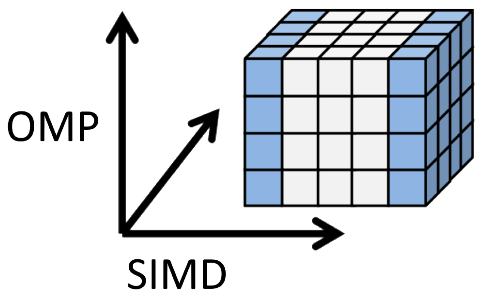
The uniform grid in the Cartesian coordinates for solving the hydrodynamical equations allows one to use arbitrary Cartesian topology for the domain decomposition. This structure of the computation provides great potential for scalability. The OMPEGAS code uses the multilevel multidimensional decomposition of the domain. On one coordinate, the inner fine decomposition is performed by vectorization, while decomposition of two other coordinates is performed by two collapsed OpenMP loops.

Note that our method also allows one to perform additional decomposition by one of the coordinates using the MPI with one layer for subdomains overlapping.

Figure 1 shows the geometric domain decomposition implemented by the OpenMP and vectorization.

3.2. OpenMP + SIMD Implementation

The following algorithm for computing the single time step is used (with the corresponding function names used in the code):

• Find a minimum time step between all spatial cells (computational_tau()).
• Construct the local parabolic approximations of primitive variables for each cell, consider the boundary conditions (build_parabola_sdlt()).
• Solve the Riemann problem for each cell (eulerian_stage()).
• Process the boundary conditions for the obtained conservative variables.
• Recover the primitive variables for each cell.
• Process the boundary conditions for the primitive variables (boundary_mesh()).

3.3. Data Structures

To optimize the data storage for the parabolic coefficients, we used the Intel SDLT library [43]. It allows one to achieve the performance of the vectorized C++ code by automatically converting the Array of Structures to the Structure of Arrays by aligning the data to the SIMD words and cache lines and providing the n-dimensional containers. The code is shown in Listing 1.

Listing 1. Declaration of data structures for the parabolic approximations.

#include <sdlt/sdlt.h>

// type of parabola

struct parabola

{

// parameters of parabola

real ulr, ull, dq, dq6, ddq;

// right integral of parabola

inline real right_parabola (real ksi, real h) const

// left integral of parabola

inline real left_parabola (real ksi, real h) const

// build local parabola

inlinevoid local_parabola (real uvalue)

// reconstruct parabola

inlinevoid reconstruct_parabola (real uvalue)

};

// type of mesh

struct mesh

{

// value on mesh

real u;

// parabols

parabola parx, pary, parz;

};

// invoking SDLT macros for structures

SDLT_PRIMITIVE(parabola, ulr, ull, dq, dq6, ddq)

SDLT_PRIMITIVE(mesh, u, parx, pary, parz)

// defining the 3D container type

typedef sdlt :: n_container <mesh, sdlt :: layout :: soa<1>, \

sdlt :: n_extent_t<int, int, int>> ContainerMesh3D;

Listing 1. Declaration of data structures for the parabolic approximations.

#include <sdlt/sdlt.h>

// type of parabola

struct parabola

{

// parameters of parabola

real ulr, ull, dq, dq6, ddq;

// right integral of parabola

inline real right_parabola (real ksi, real h) const

// left integral of parabola

inline real left_parabola (real ksi, real h) const

// build local parabola

inlinevoid local_parabola (real uvalue)

// reconstruct parabola

inlinevoid reconstruct_parabola (real uvalue)

};

// type of mesh

struct mesh

{

// value on mesh

real u;

// parabols

parabola parx, pary, parz;

};

// invoking SDLT macros for structures

SDLT_PRIMITIVE(parabola, ulr, ull, dq, dq6, ddq)

SDLT_PRIMITIVE(mesh, u, parx, pary, parz)

// defining the 3D container type

typedef sdlt :: n_container <mesh, sdlt :: layout :: soa<1>, \

sdlt :: n_extent_t<int, int, int>> ContainerMesh3D;

3.4. Auto Vectorization

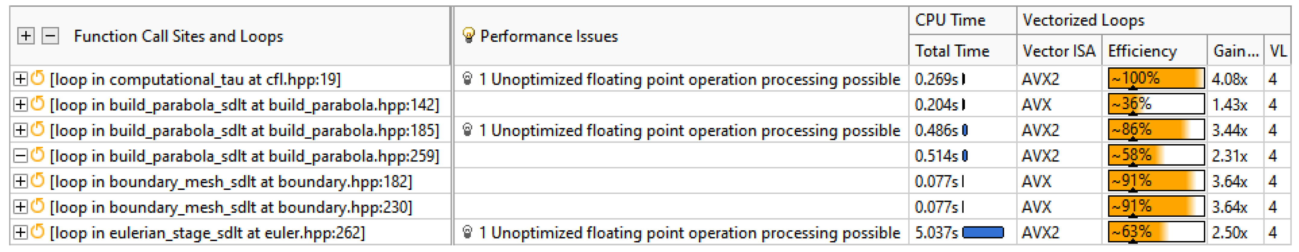
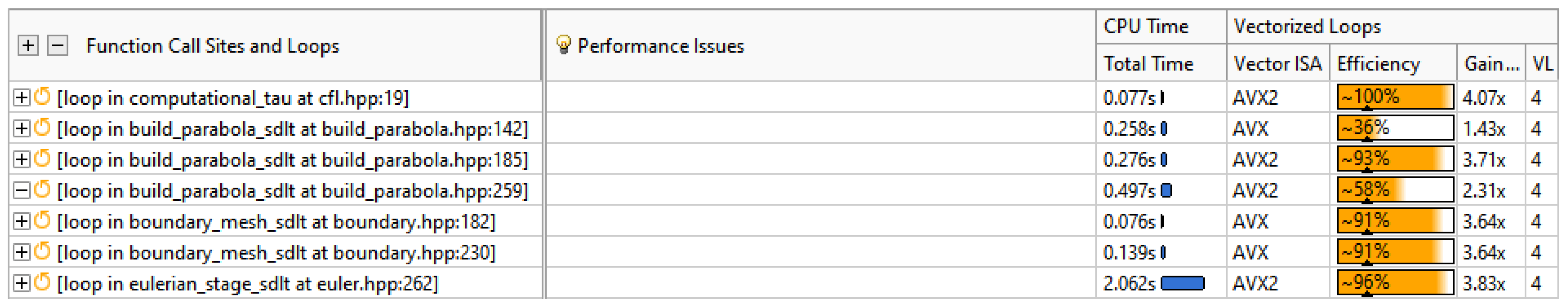
To study the code for vectorization, we used the Intel Advisor tool [44]. The initial analysis showed that the automatic vectorization was prevented due to the supposed dependencies and function calls. To avoid this, we used the directive ‘#pragma ivdep’ for loops and ‘#pragma forceinline recursive’ for functions. This allowed the compiler to vectorize automatically the relevant loops.

The next recommendation by the Advisor was optimizing the arithmetic operations. The costliest procedure of the Riemann solver performed 750 divisions in the loop body. After using the compiler option ‘\Qprec-div-’, this number was reduced approximately to 300. Figure 2 and Figure 3 show the result of the Advisor survey before and after applying this option. Note that the vectorization efficiency of the Riemann solver loop (last row) rose from 2.5 times to a nearly perfect fourfold.

The procedures for constructing the parabolic approximations [29] used a lot of branching. Thus, their vectorization potential was limited.

3.5. OpenMP Parallelization

Parallelization was performed by distributing the workload between the OpenMP threads. Listing 2 shows the typical usage of ‘#pragma omp for’ directive for the Riemann solver loop. Two outer loops were collapsed and parallelized using the OpenMP. The inner loop was vectorized. The scheduling was set to ‘runtime’, which allowed us to tune the program without recompiling.

Listing 2. Riemann solver loop.

#pragma omp for schedule (runtime) collapse (2)

for (i = 1; i < NX − 1; i++)

for (k = 1 ; k < NY − 1; k++)

#pragma ivdep

for (l = 1; l < NZ − 1; l++)

{

// Riemann solver

#pragma forceinline recursive

SRHD_Lamberts_Riemann (

…

Listing 2. Riemann solver loop.

#pragma omp for schedule (runtime) collapse (2)

for (i = 1; i < NX − 1; i++)

for (k = 1 ; k < NY − 1; k++)

#pragma ivdep

for (l = 1; l < NZ − 1; l++)

{

// Riemann solver

#pragma forceinline recursive

SRHD_Lamberts_Riemann (

…

3.6. Code Research

The numerical experiments were performed on a 16-core Intel Core i9-12900K processor with AVX/AVX2 support and DDR5-6000 memory. A mesh with the size of $128 \times 128 \times 128$ was used to solve the evaluation. The computing times presented below exclude the time spent on the initialization, finalizing, and file operations.

3.6.1. Performance of Single Thread Using Vectorization

Table 1. Results of the auto-vectorization and division optimization.

SIMD Length	Time [Minutes]
	Precise Division	Optimized Division
No vectorization	25	14
$4\times$ double (AVX2)	13.3	7.6

shows the computing time of a single-threaded program with various compilation settings. To disable auto-vectorization, we used the \Qvec- option, and to use the precise or optimized divisions, we used the \Qprec-div or \Qprecc-div-, respectively.

3.6.2. Threading Performance

For studying the threading performance, we used the speedup $S_m=T_1/T_m$ coefficient, where $T_m$ is the calculation time on m threads for the same problem.

Table 2. Threading performance for the test problem.

Number m of OpenMP Threads	Time ${\mathit{T}}_{\mathit{m}}$ [Minutes]	Speedup ${\mathit{S}}_{\mathit{m}}$	Memory Bandwidth Utilization [GB/s]	Performance [GFLOPs]
1 (Serial)	7.6	—	19	16
2	4.8	1.6	31	26
4	3.4	2.27	48	39
8	3.0	2.53	59	47
16	2.9	2.64	70	49
24	2.9	2.61	65	48
Hardware maximum			88	856

shows the results of solving the problem with the $128 \times 128 \times 128$ mesh on various numbers of the OpenMP threads. The table contains the computing time of the program and speedup for various numbers of the OpenMP threads. It also shows the memory bandwidth utilization and performance in FLOPs, as well as the maximum values obtained via the Intel Advisor. Note that these two values were affected by the profiling overhead.

4. Discussion

In this section, we define several important (as we see it) aspects that were not noted above. In the present case, these issues were not primarily important, but they will be addressed in further works.

• In this work, we used the statement of the special relativistic hydrodynamical model in the form of the mass, moment, and total mechanical energy conservation laws. This did not take into account the magnetic fields. In the future, we may implement the magnetohydrodynamical model.
• The Core i9-12900K CPU is based on heterogeneous architecture. It included 8 high-performance cores and 8 power-efficient cores. In future, such systems will probably gain more popularity. One of the problems was the difference in performance between cores resulting in the thread imbalance. For our code changing the OpenMP scheduling from ‘static’ to the ‘dynamic,1’, reduced the execution time from 185 to 176 s, an improvement of 5%. Note that while the high-performance cores support the Hyper-Threading (allowing the CPU to run 24 hardware threads), the best results are achieved by the 16 OpenMP threads.
• Another challenge was in the fact that the implementation was memory-bound. We investigated the performance of the most costly procedure, namely, the Riemann solver.

  Table 3. Performance of the Riemann solver.

  Number m of OpenMP Threads	Memory Bandwidth Utilization [GB/s]	Performance [GFLOPs]
  1 (Serial)	12	27
  2	24	50
  4	37	78
  8	52	110
  16	70	121
  24	65	114
  Hardware maximum	88	856

  presents the memory bandwidth utilization and performance in the GFLOPS for the parallel implementation of this procedure with various numbers of OpenMP threads. The values were obtained by Intel Advisor.
  The table shows that the performance was limited by the memory bandwidth. The roofline analysis by the Intel Advisor (presented in Figure 4) confirmed that the implementation was bound mostly by the memory.
  There are several ways to overcome this problem.
  • Utilize hardware with a higher memory bandwidth, such as graphics processors. Modern GPUs’ memory bandwidth is usually much higher than that in CPUs.
  • Use distributed memory systems. This approach would provide the effective summation of the bandwidths of the individual computers. It would also allow one to solve larger problems that do not fit into a single unit. Our numerical method and the domain decomposition approach provide an efficient way to implement the MPI parallelization.
  • The OmpSs programming model [45] may be used to develop parallel code for heterogeneous computing systems with CPUs and GPUs.
  • Increase the arithmetic intensity of the code. This may be achieved by using higher-order numerical methods.
  • Application of specialized data structures tailored for the task. For example, the Locally Recursive non-Locally Asynchronous algorithms with the Functionally Arranged Shadow structure [46] provide better cache reuse and arithmetic intensity for stencil methods than the classic nested loop traversal.

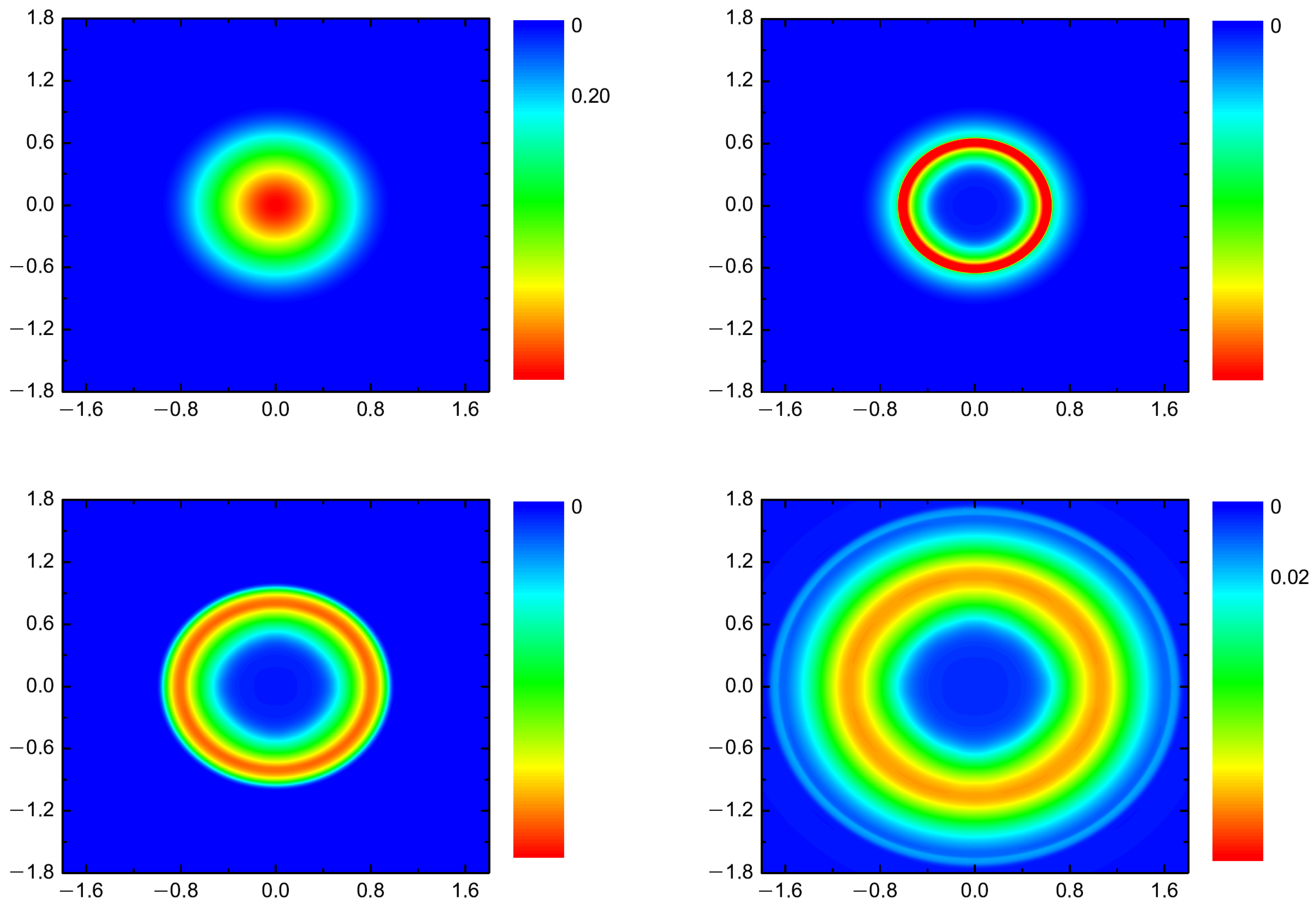
5. Model Problem: Hydrodynamical Simulation of Star Explosion

Let us consider the model problem of a hydrodynamical explosion. At the center of the star (defined by the equilibrium density profile), we induce the point blast with a given dispersion of the density $\delta \rho /\rho \approx$ 2%. Further, all equations and results of the simulation are presented in the dimensionless form.

As the initial data for the profile of the star, let us take ones of the hydrostatic equilibrium configuration. In spherical coordinates with the gravitational constant $G\equiv 1$, the data have the form

$$\frac{\partial p}{\partial r}=-\frac{M\left(r\right)\rho }{r^2},$$

$$\frac{\partial M}{\partial r}=4\pi r^2\rho .$$

The initial density distribution is chosen as follows:

$${\rho }_0\left(r\right)=\left\{\begin{array}{cc}\hfill 1-r,& \hfill r\le 1,\\ \hfill 0,& \hfill r>1.\end{array}\right.$$

Thus, the initial distribution of the pressure and gravitational potential have the form

$$p_0\left(r\right)=\left\{\begin{array}{cc}\hfill -\frac{\pi r^2}{36}(9r^2-28r+24)+\frac{5\pi }{36},& \hfill r\le 1,\\ \hfill 0,& \hfill r>1,\end{array}\right.$$

$${\Phi }_0\left(r\right)=\left\{\begin{array}{cc}\hfill -\frac{\pi }{3}(r^3-2r^2)-\frac{2\pi }{3},& \hfill r\le 1,\\ \hfill -\frac{\pi }{3r},& \hfill r>1.\end{array}\right.$$

We shall use this profile to define the initial configuration of the star.

Figure 5 shows the results of the simulation and the density profiles at various instants.

Despite introducing the random perturbations of the star, the physics was dominated by the process of the point blast similar to the Sedov problem.

6. Conclusions

We presented a novel hydrodynamic OMPEGAS code for the three-dimensional simulation of astrophysical flows using multicore processors with vector instructions. By using auto-vectorization, we achieved a 3.3-fold increase in speed in comparison with the non-vectorized program on a processor with AVX2 support. By using multithreading with the OpenMP, we achieved an increase in speed of 2.6 times on a 16-core processor in comparison with the vectorized single-threaded program. In the total, an increase in speed of nearly nine times was achieved for the test problem. The numerical experiment was performed for the model problem of the hydrodynamical simulation of a star explosion.

References

1. Tutukov, A.V.; Cherepashchuk, A.M. Evolution of close binary stars: Theory and observations. Physics-Uspekhi 2020, 63, 209. [Google Scholar] [CrossRef]
2. Tutukov, A.V.; Dryomova, G.N.; Dryomov, V.V. Hypervelocity stars: Theory and observations. Physics-Uspekhi 2021, 64, 967. [Google Scholar] [CrossRef]
3. Mezcua, M. Dwarf galaxies might not be the birth sites of supermassive black holes. Nat. Astron. 2019, 3, 6–7. [Google Scholar] [CrossRef]
4. Miceli, M.; Orl, O.S.; Burrows, D.N.; Frank, K.A.; Argiroffi, C.; Reale, F.; Peres, G.; Petruk, O.; Bocchino, F. Collisionless shock heating of heavy ions in SN 1987A. Nat. Astron. 2019, 3, 236–241. [Google Scholar] [CrossRef] [Green Version]
5. Mitchell, N.; Vorobyov, E.; Hensler, G. Collisionless Stellar Hydrodynamics as an Efficient Alternative to N-body Methods. Mon. Not. R. Astron. Soc. 2013, 428, 2674–2687. [Google Scholar] [CrossRef] [Green Version]
6. Kulikov, I. GPUPEGAS: A New GPU-accelerated Hydrodynamic Code for Numerical Simulations of Interacting Galaxies. Astrophys. J. Suppl. Ser. 2014, 214, 1–12. [Google Scholar] [CrossRef] [Green Version]
7. Pabst, C.; Higgins, R.; Goicoechea, J.R.; Teyssier, D.; Berne, O.; Chambers, E.; Wolfire, M.; Suri, S.T.; Guesten, R.; Stutzki, J.; et al. Disruption of the Orion molecular core 1 by wind from the massive star θ1 Orionis C. Nature 2019, 565, 618–621. [Google Scholar] [CrossRef]
8. Forbes, J.; Krumholz, M.; Goldbaum, N.; Dekel, A. Suppression of star formation in dwarf galaxies by photoelectric grain heating feedback. Nature 2016, 535, 523–525. [Google Scholar] [CrossRef]
9. Willcox, D.; Townsley, D.; Calder, A.; Denissenkov, P.; Herwig, F. Type Ia supernova explosions from hybrid carbon–oxygen–neon white dwarf progenitors. Astrophys. J. 2016, 832, 13. [Google Scholar] [CrossRef] [Green Version]
10. Spillane, T.; Raiola, F.; Rolfs, C.; Schürmann, D.; Strieder, F.; Zeng, S.; Becker, H.W.; Bordeanu, C.; Gialanella, L.; Romano, M.; et al. 12C + 12C Fusion Reactions near the Gamow Energy. Phys. Rev. Lett. 2007, 98, 122501. [Google Scholar] [CrossRef] [Green Version]
11. Jiang, J.A.; Maeda, K.; Shigeyama, T.; Nomoto, K.I.; Yasuda, N.; Jha, S.W.; Tanaka, M.; Morokuma, T.; Tominaga, N.; Ivezić, Ž.; et al. A hybrid type Ia supernova with an early flash triggered by helium-shell detonation. Nature 2017, 550, 80–83. [Google Scholar] [CrossRef] [PubMed] [Green Version]
12. Kulikov, I.; Chernykh, I.; Karavaev, D.; Protasov, V.; Serenko, A.; Prigarin, V.; Ulyaniche, I.; Tutukov, A. Using Adaptive Nested Mesh Code HydroBox3D for Numerical Simulation of Type Ia Supernovae: Merger of Carbon-Oxygen White Dwarf Stars, Collapse, and Non-Central Explosion. In Proceedings of the 2018 Ivannikov ISP RAS Open Conference ISPRAS 2018, Moscow, Russia, 22–23 November 2018; pp. 77–81. [Google Scholar] [CrossRef]
13. Terreran, G.; Pumo, M.L.; Chen, T.W.; Moriya, T.J.; Taddia, F.; Dessart, L.; Zampieri, L.; Smartt, S.J.; Benetti, S.; Inserra, C.; et al. Hydrogen-rich supernovae beyond the neutrino-driven core-collapse paradigm. Nat. Astron. 2017, 1, 713–720. [Google Scholar] [CrossRef]
14. Mendygral, P.J.; Radcliffe, N.; Kandalla, K.; Porter, D.; O’Neill, B.J.; Nolting, C.; Edmon, P.; Donnert, J.M.; Jones, T.W. WOMBAT: A Scalable and High-performance Astrophysical Magnetohydrodynamics Code. Astrophys. J. Suppl. Ser. 2017, 228, 23. [Google Scholar] [CrossRef] [Green Version]
15. Schneider, E.; Robertson, B. Cholla: A new massively parallel hydrodynamics code for astrophysical simulation. Astrophys. J. Suppl. Ser. 2015, 217, 24. [Google Scholar] [CrossRef] [Green Version]
16. Schneider, E.; Robertson, B. Introducing CGOLS: The Cholla Galactic Outflow Simulation Suite. Astrophys. J. 2018, 860, 135. [Google Scholar] [CrossRef] [Green Version]
17. Schneider, E.; Robertson, B.; Thompson, T. Production of Cool Gas in Thermally Driven Outflows. Astrophys. J. 2018, 862, 56. [Google Scholar] [CrossRef]
18. Collela, P. Multidimensional Upwind Methods for Hyperbolic Conservation Laws. J. Comput. Phys. 1990, 87, 171–200. [Google Scholar] [CrossRef] [Green Version]
19. Gardiner, T.; Stone, J. An unsplit Godunov method for ideal MHD via constrained transport in three dimensions. J. Comput. Phys. 2008, 227, 4123–4141. [Google Scholar] [CrossRef] [Green Version]
20. Schive, H.; Tsai, Y.; Chiueh, T. GAMER: A GPU-accelerated Adaptive-Mesh-Refinement Code for Astrophysics. Astrophys. J. 2010, 186, 457–484. [Google Scholar] [CrossRef] [Green Version]
21. Schive, H.; ZuHone, J.; Goldbaum, N.; Turk, M.; Gaspari, M.; Cheng, C. GAMER-2: A GPU-accelerated adaptive mesh refinement code—Accuracy, performance, and scalability. Mon. Not. R. Astron. Soc. 2018, 481, 4815–4840. [Google Scholar] [CrossRef] [Green Version]
22. Zhang, U.; Schive, H.; Chiueh, T. Magnetohydrodynamics with GAMER. Astrophys. J. Suppl. Ser. 2018, 236, 50. [Google Scholar] [CrossRef] [Green Version]
23. Benitez-Llambay, P.; Masset, F. FARGO3D: A new GPU-oriented MHD code. Astrophys. J. Suppl. Ser. 2016, 223, 11. [Google Scholar] [CrossRef] [Green Version]
24. Griffiths, M.; Fedun, V.; Erdelyi, R. A Fast MHD Code for Gravitationally Stratified Media using Graphical Processing Units: SMAUG. J. Astrophys. Astron. 2015, 36, 197–223. [Google Scholar] [CrossRef] [Green Version]
25. Kulikov, I.M.; Chernykh, I.G.; Snytnikov, A.V.; Glinskiy, B.M.; Tutukov, A.V. AstroPhi: A code for complex simulation of dynamics of astrophysical objects using hybrid supercomputers. Comput. Phys. Commun. 2015, 186, 71–80. [Google Scholar] [CrossRef]
26. Kulikov, I.M.; Chernykh, I.G.; Glinskiy, B.M.; Protasov, V.A. An Efficient Optimization of HLL Method for the Second Generation of Intel Xeon Phi Processor. Lobachevskii J. Math. 2018, 39, 543–550. [Google Scholar] [CrossRef]
27. Popov, M.; Ustyugov, S. Piecewise parabolic method on local stencil for gasdynamic simulations. Comput. Math. Math. Phys. 2007, 47, 1970–1989. [Google Scholar] [CrossRef]
28. Popov, M.; Ustyugov, S. Piecewise parabolic method on a local stencil for ideal magnetohydrodynamics. Comput. Math. Math. Phys. 2008, 48, 477–499. [Google Scholar] [CrossRef]
29. Kulikov, I.; Vorobyov, E. Using the PPML approach for constructing a low-dissipation, operator-splitting scheme for numerical simulations of hydrodynamic flows. J. Comput. Phys. 2016, 317, 318–346. [Google Scholar] [CrossRef] [Green Version]
30. Kulikov, I.M.; Chernykh, I.G.; Tutukov, A.V. A New Parallel Intel Xeon Phi Hydrodynamics Code for Massively Parallel Supercomputers. Lobachevskii J. Math. 2018, 39, 1207–1216. [Google Scholar] [CrossRef]
31. Kulikov, I. A new code for the numerical simulation of relativistic flows on supercomputers by means of a low-dissipation scheme. Comput. Phys. Commun. 2020, 257, 107532. [Google Scholar] [CrossRef]
32. Pandolfi, M.; D’Ambrosio, D. Numerical instabilities in upwind methods: Analysis and cures for the “carbuncle” phenomenon. J. Comput. Phys. 2000, 166, 271–301. [Google Scholar] [CrossRef] [Green Version]
33. Chauvat, Y.; Moschetta, J.-M.; Gressier, J. Shock wave numerical structure and the carbuncle phenomenon. Int. J. Numer. Methods Fluids 2005, 47, 903–909. [Google Scholar] [CrossRef] [Green Version]
34. Liou, M.S. Mass flux schemes and connection to shock instability. J. Comput. Phys. 2000, 160, 623–648. [Google Scholar] [CrossRef]
35. Xu, K.; Li, Z. Dissipative mechanism in Godunov-type schemes. Int. J. Numer. Methods Fluids 2001, 37, 1–22. [Google Scholar] [CrossRef]
36. Kim, S.-S.; Kim, C.; Rho, O.-H.; Hong, S.K. Cures for the shock instability: Development of a shock-stable Roe scheme. J. Comput. Phys. 2003, 185, 342–374. [Google Scholar] [CrossRef]
37. Dumbser, M.; Morschetta, J.-M.; Gressier, J. A matrix stability analysis of the carbuncle phenomenon. J. Comput. Phys. 2004, 197, 647–670. [Google Scholar] [CrossRef] [Green Version]
38. Davis, S.F. A rotationally biased upwind difference scheme for the Euler equations. J. Comput. Phys. 1984, 56, 65–92. [Google Scholar] [CrossRef] [Green Version]
39. Levy, D.W.; Powell, K.G.; van Leer, B. Use of a rotated Riemann solver for the two-dimensional Euler equations. J. Comput. Phys. 1993, 106, 201–214. [Google Scholar] [CrossRef] [Green Version]
40. Ren, Y.-X. A robust shock-capturing scheme based on rotated Riemann solvers. Comput. Fluids 2003, 32, 1379–1403. [Google Scholar] [CrossRef]
41. Nishikawa, H.; Kitamura, K. Very simple, carbuncle-free, boundary-layer-resolving, rotated-hybrid Riemann solvers. J. Comput. Phys. 2008, 227, 2560–2581. [Google Scholar] [CrossRef]
42. Kulikov, I.; Chernykh, I.; Tutukov, A. A New Hydrodynamic Code with Explicit Vectorization Instructions Optimizations that Is Dedicated to the Numerical Simulation of Astrophysical Gas Flow. I. Numerical Method, Tests, and Model Problems. Astrophys. J. Suppl. Ser. 2019, 243, 1–15. [Google Scholar] [CrossRef]
43. Intel Corporation. SIMD Data Layout Templates. Available online: https://www.intel.com/content/www/us/en/develop/documentation/oneapi-dpcpp-cpp-compiler-dev-guide-and-reference/top/compiler-reference/libraries/introduction-to-the-simd-data-layout-templates.html (accessed on 23 February 2022).
44. Intel Corporation. Intel Advisor User Guide. Available online: https://www.intel.com/content/www/us/en/develop/documentation/advisor-user-guide/top.html (accessed on 23 February 2022).
45. Programming Models Group BSC. OmpSs-2 Programming Model. Available online: https://pm.bsc.es/ompss-2 (accessed on 14 July 2022).
46. Perepelkina, A.; Levchenko, V.D. Functionally Arranged Data for Algorithms with Space-Time Wavefront. In Proceedings of the Parallel Computational Technologies, PCT 2021, Communications in Computer and Information Science, Volgograd, Russia, 30 March–1 April 2021; Volume 1437. [Google Scholar] [CrossRef]
Figure 1. Geometric domain decomposition.
Mathematics 10 02546 g001
Figure 2. Intel Advisor vectorization survey for the original code.
Mathematics 10 02546 g002
Figure 3. Intel Advisor vectorization survey for the optimized division.
Mathematics 10 02546 g003
Figure 4. Intel Advisor Roofline Analysis graph for the Riemann Solver procedure.
Mathematics 10 02546 g004
Figure 5. Density of the supernova in the equatorial cut of the star at the dimensionless instants of time 0 (top left), 0.1 (top right), 0.2 (bottom left), and 0.4 (bottom right).
Mathematics 10 02546 g005