
Knowledge-Based Scene Graph Generation with Visual Contextual Dependency


1
School of Computer Science and Engineering, University of Electronic Science and Technology of China, Chengdu 611731, China
2
School of Information and Software Engineering, University of Electronic Science and Technology of China, Chengdu 611731, China
3
Research Institute of Social Development, Southwestern University of Finance and Economics, Chengdu 611130, China
*
Authors to whom correspondence should be addressed.
†
These authors contributed equally to this work.
Mathematics 2022, 10(14), 2525; https://doi.org/10.3390/math10142525
Submission received: 18 June 2022
/
Revised: 7 July 2022
/
Accepted: 13 July 2022
/
Published: 20 July 2022
(This article belongs to the Special Issue Trustworthy Graph Neural Networks: Models and Applications)
Abstract
:Scene graph generation is the basis of various computer vision applications, including image retrieval, visual question answering, and image captioning. Previous studies have relied on visual features or incorporated auxiliary information to predict object relationships. However, the rich semantics of external knowledge have not yet been fully utilized, and the combination of visual and auxiliary information can lead to visual dependencies, which impacts relationship prediction among objects. Therefore, we propose a novel knowledge-based model with adjustable visual contextual dependency. Our model has three key components. The first module extracts the visual features and bounding boxes in the input image. The second module uses two encoders to fully integrate visual information and external knowledge. Finally, visual context loss and visual relationship loss are introduced to adjust the visual dependency of the model. The difference between the initial prediction results and the visual dependency results is calculated to generate the dependency-corrected results. The proposed model can obtain better global and contextual information for predicting object relationships, and the visual dependencies can be adjusted through the two loss functions. The results of extensive experiments show that our model outperforms most existing methods.
Keywords:
scene graph generation; external knowledge; context fusion; computer vision; visual dependency constraintMSC:
68T071. Introduction
Scene graph generation (SGG) [1] aims to detect objects and their relationships in images. The generated scene graphs capture rich semantic information in the images and can be used to extend knowledge beyond individual objects. Therefore, SGG can provide significant assistance for subsequent computer vision [1,2,3,4,5,6] and scene understanding [7,8,9,10,11] tasks.
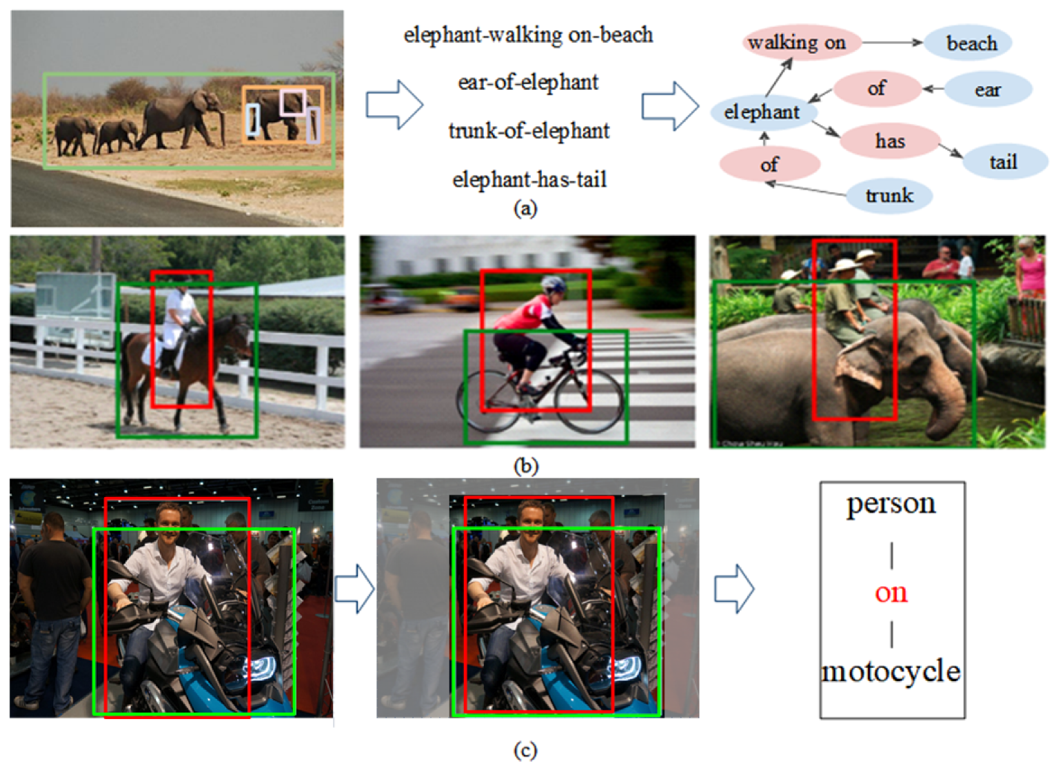
Early studies on SGG relied solely on visual contextual information to identify object relationships in images [12,13,14,15]. These methods successively pass visual features through a given network to update the feature representations and relationships of different objects. However, because scenes may include diverse visual relationships, simple visual features cannot fully represent the contextual information contained in a scene. For example, in the images shown in Figure 1, the relationships, (person, ride, horse) and (person, ride, bicycle), are semantically similar. However, horses and bicycles have considerably different appearances in the images, and an SGG model should use external knowledge to infer that these relationships are the same. Thus, methods that rely solely on visual contextual information are inadequate for SGG.
Recently, external knowledge, including inter-object statistical information and common-sense information [13,16,17,18], has been incorporated into SGG tasks through two related approaches. The first method uses the inter-object statistical information to initialize the edge weights in the graph structure. For example, Chen et al. [19] used statistical correlations between object pairs to construct message-passing graphs. However, this approach failed to fully exploit the semantic content of the statistical information. In fact, this approach mainly uses visual information and does not deeply mine external knowledge. The second method uses external knowledge and visual information to construct common-sense graphs for predicting object relationships. For example, Zareian et al. [20] constructed a common-sense graph and used connections in the knowledge and scene graphs to represent objects and their relationships. These methods incorporate visual features and categorical information into the nodes of knowledge graphs and update the nodes and relational representations by propagating messages through the graph. However, visual context is crucial in relational reasoning, and both knowledge-based approaches fail to combine the visual information contained in the images with the rich semantic information provided by external knowledge when predicting object relationships.
In summary, two essential tasks should be considered when incorporating external knowledge. The first task that should be considered is how the external knowledge and visual features should be combined to best learn the global contextual information contained in a scene. Visual and contextual semantic features can both assist models in accurately predicting object relationships. Therefore, an important challenge is developing a method for combining these two types of features that comprehensively captures the underlying information. The second task is how the model’s reliance on visual information and external knowledge should be adjusted. As shown in Figure 1, when the same relationship has various possible visual features (such as <man, ride, horse> and <man, ride, bicycle>), visual information plays a major role in relationship prediction. However, when a relationship is represented by only a few samples in a dataset, the relationship must be inferred according to external knowledge. Therefore, a high-level SGG model must not only fully integrate effective information from visual features and external knowledge but also adjust the dependence of the model on these two information sources.
In this paper, we propose a novel knowledge-based SGG model with visual contextual dependency (KVCD). Our KVCD model combines external knowledge and visual features to determine the global contextual information in a scene. Furthermore, because our model learns and adjusts visual dependencies during the fusion process, our model can generate more balanced scene graphs. The proposed model includes three modules. First, the feature extraction module uses object detection to determine the visual features contained in an image. Second, the relational reasoning module uses the visual features extracted by the previous module and applies a novel approach to combine external knowledge with these visual features. This module uses two encoders to obtain the global contextual information. The first encoder corrects the initial object classification results using an external knowledge base. Then, the second encoder encodes the semantic features and external knowledge obtained in the previous layer. Thus, the model can generate richer contextual information than previous models. As a result, our model can fully use external knowledge as auxiliary information to supplement the visual feature information for SGG. Finally, the visual dependency constraint module applies two losses (the visual context loss and the visual relationship loss) to balance the model’s reliance on the two types of knowledge applied in the relational reasoning module. The performance of the model is validated with the Visual Genome dataset, and the results show that our model outperforms most existing approaches. The contributions of this paper can be summarized as follows:
- To ensure that external knowledge is fully utilized, we propose a novel SGG method based on visual–semantic context fusion. We design two encoder–decoder bidirectional long short-term memory (BiLSTM) networks that successively update the visual and contextual information according to the external knowledge.
- To address the dependencies caused by introducing external knowledge and datasets, we propose two loss functions (the visual loss and visual context loss) to learn the model’s bias towards the external knowledge and contextual information. By analysing the effect of these two dependencies on the results, our model can generate more effective scene graphs.
- Our model is extensively evaluated, and the results show the advantages of the proposed model over comparative baselines in terms of the Recall@K and mean Recall@K metrics.
The remainder of this paper is organized as follows. In Section 2, we briefly introduce relevant research on information transmission-based and external knowledge-based SGG. In Section 3, we discuss the main structures of the proposed SGG method, which is based on the fusion of visual and semantic context information, and our baseline model. In Section 4, we present the experimental results and comparisons with previous models. In Section 5, we conclude this work.
2. Related Work
SGG involves determining the representations of objects and their relationships in visual scenes. In recent years, various works have investigated visual scenes in images. Li et al. [21] proposed the multilevel scene description network (MSDN) model and explored the possibility of using a single neural network to understand images from three perspectives: object detection, SGG, and image captioning. Inspired by the knowledge base, Zhang et al. proposed VTransE [22], an extension of the TransE [23] method of visual relationship detection. Dai et al. proposed deep relational networks (DR-Net) [24] based on deep neural networks for jointly predicting category labels according to the spatial configurations and statistical correlations of various targets. Image contextual information has also received attention from researchers. For example, Newell et al. proposed Pixels2Graphs [25], an approach that uses the image’s context to jointly reason the relational labels for an entire scene graph. Wang et al. [26] adopted a method that first prioritized the key relationships in a scene and then identified trivial relationships to obtain a complete scene graph. Recent works, including information-transmission-based and external knowledge-based methods, have focused on learning visual knowledge in SGG tasks.
Information transmission-based methods. Joint reasoning based on contextual information fully considers the semantic information contained in an image to generate a complete scene-graph representation. Inspired by this approach, Li et al. [27] decomposed connectivity graphs between targets into sub-graphs with a top-down clustering method and refined the sub-graph features using a spatially weighted message-passing method to generate the scene graph. To better capture the contextual information, Herzig et al. [28] proposed an alignment-invariant structure prediction SGG approach that identifies visual scenes with multiple interrelated objects according to the global context. Woo et al. proposed the LinkNet [29] model, which is based on the interdependencies between object instances. Zellers et al. proposed a global context method for SGG based on the concept of neural motifs [15]. Due to the fact that the neural motif method uses local visual relationships and the contextual information of the entire image, this method can generate more complete feature representations. Xu et al. proposed an iterative message-passing (IMP) method [14] that iteratively transmits contextual information about objects and their relationships. Tang et al. proposed a visual context tree (VCTree) model [12]. In contrast to the IMP and neural motif methods, the VCTree model uses a tree structure to extract the features of object nodes and relation edges. However, because the detection of predicates requires that each pair of target proposals be enumerated, the VCTree model has considerable computational complexity. Zareian et al. [30] proposed a visual–semantic parsing network (VSPNET) that uses novel vector space-planning methods to map entity nodes and edges to semantic spaces. VSPNET decreases its computational complexity by generating vector space mappings.
However, these information-transmission-based approaches utilize the visual features in an iterative manner and do not use external information to assist in reasoning on scene graphs. Therefore, these models are susceptible to visual dependencies when relationship categories with a large number of samples are used. Furthermore, the performance of these models is reduced when relationship categories with a small number of samples are employed.
External knowledge-based methods. In addition to visual contextual information, many researchers have focused on identifying effective external knowledge (e.g., language priors and knowledge graphs). The knowledge-embedded routing network (KERN) model [19] considers the statistical correlations between object pairs as language priors. These language priors can assist the object detection network in predicting object classes and determining the graphical structure of the identified objects and relationships. The KERN model uses this graphical structure to infer relationships and generate scene graphs. To address the long-tail problem associated with object and relationship distributions in SGG datasets, Gu et al. proposed KB-GAN [31]. KB-GAN uses external knowledge to refine the target and predicate features and generates scene graphs through a generative adversarial network (GAN)-based approach. The graph-bridging network (GB-NET) model [20] transforms scene graphs into knowledge graphs to better identify visual relations. Although the introduction of external knowledge improves the model’s performance on SGG tasks, the deviations caused by long-tailed distributions in category datasets with a small number of samples and the issues associated with joint analyses with visual features when generating complete scene graphs still need to be resolved.
In addition to the previous method, considering the effectiveness of graph neural networks for fusing contextual information, Yang et al. proposed the Graph R-CNN [32] method for calculating correlation scores among objects and removing unlikely relationships. Qi et al. [33] embedded joint graphical representations by introducing an attention mechanism. In addition, an effective loss function can improve the SGG performance. Moreover, Zhang et al. [34] introduced the graphical contrast loss to address the issue of pairing the same predicate with different instances. Chen et al. [35] used the cross-entropy as a loss function for target detection and optimized SGG through a multi-agent strategy.
3. Methodology
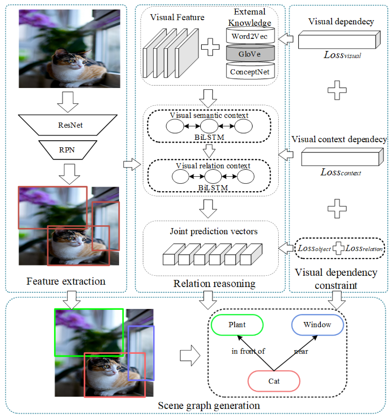
An overview of our proposed model is shown in Figure 2. The various components are introduced in detail in the following sections. Our model can be summarized in three steps:
- Feature extraction. The object features, bounding boxes, and class distributions in the input image are extracted by the feature-extraction module.
- Relational reasoning. The relational reasoning module identifies the corresponding word vector in the knowledge base by using the object’s visual information. To fully utilize the external knowledge, a successive updating strategy and two BiLSTM encoders are used to fuse the word vectors and visual context information.
- Visual dependency constraint. The visual relationship and visual context loss functions are introduced to learn and adjust the visual dependencies in the model.
The objectives of SGG are to detect objects in an image, to identify the relationships between object pairs, and to use graph structures to visualize these objects and their relationships. Let the target set in the image be defined as , and let the set of bounding boxes corresponding to these targets be , where N is the total number of object categories in the dataset. The set of relationships among these objects is defined as , where K is the total number of relationship categories between object pairs in the dataset. Thus, the scene graph is jointly represented by the object and relationship sets as follows: . The task of generating the scene graph can be expressed as
where is the initial probability of each target, and is the relationship between object i and object j.
3.1. Feature Extraction
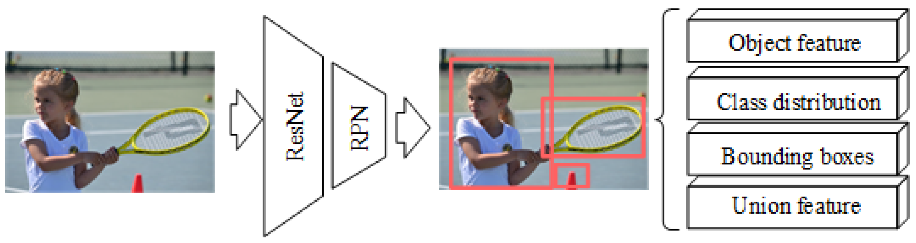
As shown in Figure 3, in the feature-extraction module, the feature map of the input image is first extracted by the backbone object-detection network, which has a residual block structure (ResNet). Then, the feature map is input into a region proposal network (RPN) to generate a set of candidate regions. Next, we apply RoIAlign to align the features and pixels in the image to obtain feature representations for each object. Thus, we can use the feature-extraction module to obtain the object features, union features, bounding boxes, and class distributions contained in the image. Finally, this module outputs visual and spatial information, which is then used by the relational reasoning module.
3.2. Relational Reasoning
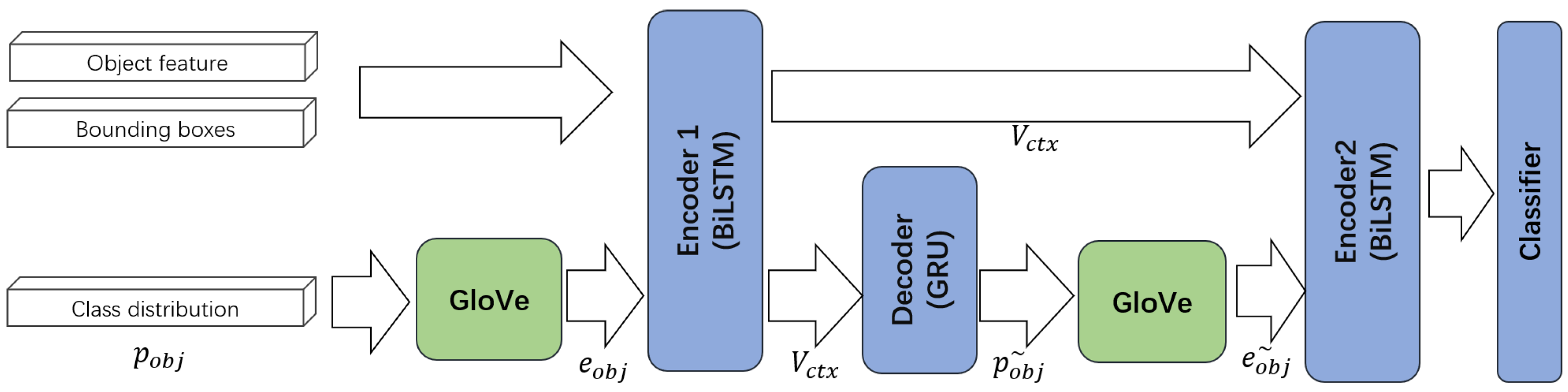
The relational reasoning module fuses external knowledge with the visual and spatial information provided by the feature-extraction module to obtain the visual–semantic context. As shown in Figure 4, we designed two encoders to fuse the external knowledge with the visual features obtained in the previous module and to incorporate the semantic information contained in the external knowledge. In the first encoder, the initial object classification results are corrected using an external knowledge base. In the second encoder, the semantic features and external knowledge extracted by the previous layer are encoded, resulting in richer contextual information than previous models.
In this paper, we define the external knowledge of different organizational approaches as the knowledge base (). Since the external knowledge contains substantial noise, we use the object category with the highest confidence to extract valid information from the . The process of extracting this external information can be expressed as:
where is the initial probability distribution of the objects identified by the object-detection network, and is a self-defined function that determines the subscript of the maximum value in and converts this value into a one-hot code according to the dimensionality of . This one-hot encoding is used to identify the corresponding word vector in the knowledge base. The includes word vectors that were generated using different organizational methods. Specifically, our relational reasoning module uses Word2Vec [36,37], GloVe [38], and ConceptNet [39] word vectors as external knowledge, and the word vector dimension is 300.
Next, the visual information and word vectors are used to fuse the context of the visual–semantic features with a BiLSTM encoder network. The visual–semantic context is decoded by a gated recurrent unit (GRU), yielding a new probability distribution. We use this probability distribution and the function to determine the final class . Thus, the final classification of the target is determined by . We obtain the target classification as follows:
where includes the image features obtained by the feature-extraction module, is the image coordinate information, and contains the union area features (the features of the union area between the target and the bounding box). It should be noted that is a 128-dimensional vector that is obtained by a fully connected layer.
Finally, we successively update using the new word vector and the second encoder network. The visual–semantic features and joint regional features of the object pair are combined, yielding the relational context features . Each object pair is classified according to the relationship context characteristics. The relationship between each object pair is classified as
where and represent the updated visual–semantic vectors of targets i and j, respectively, and represents the joint regional features. A BiLSTM network is used to combine the visual–semantic features of the object and the external knowledge, yielding vector , which contains richer contextual information than vectors generated by previous models. The second external knowledge fusion is applied to ensure that all relevant information is fully used.
3.3. Visual Dependency Constraint
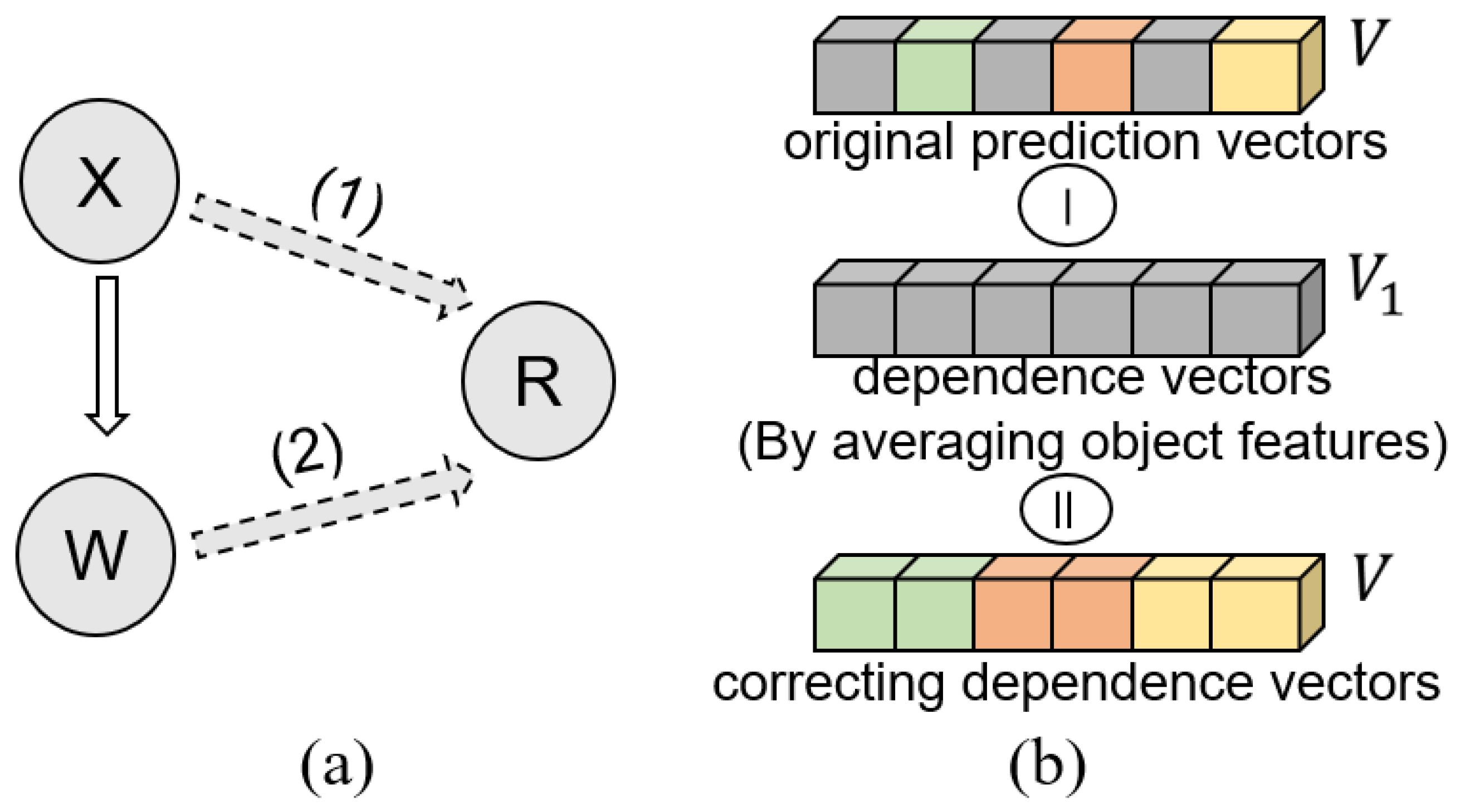
The introduction of external knowledge allows the model to identify more relationships, and the training process fits the data according to this knowledge, improving the relationship classification results. However, this approach results in model dependencies, and the relationships are predicted based on only the type of object rather than the visual information contained in the images. Therefore, the visual dependency constraint module, which applies the visual relationship loss and visual context loss functions to adjust the visual dependency of the model, is introduced. As shown in Figure 5, we input the object features contained in the image and the contextual information contained in the external knowledge into the relational reasoning module to generate an initial prediction vector. Then, we calculate the average value of the effective object features (visual features and contextual information) and use the same method to obtain a dependence vector . In , some of the effective information is removed by averaging the visual features and contextual information. Therefore, we can apply to learn the visual dependencies of the model. Finally, represents the dependency-corrected vector. To reduce possible dependencies, we design two loss functions to adjust the visual dependencies of the model, which are specified below.
Visual relationship loss. The visual relationship loss considers the dependence of the learned model on the visual object features. In an SGG task, the features () of the joint region of a target pair are usually used as the visual relationship features. Therefore, we first pass these visual features through a fully connected (FC) layer; then, we use a softmax function to predict the probabilities of these visual features and determine their relationship. Thus, the visual relationship loss can be formulated as
where K represents the number of relationship categories, represents the true target-category label value, and represents the predicted target relationship value.
Visual context loss. The visual context loss considers the dependence of the learned model on the object’s contextual information. The visual context loss is calculated in terms of the visual contextual information and the dependence of the learned model on this visual information. First, the learned visual context features are passed through an FC layer, as shown in Equation (6); then, a softmax function is used to calculate the probability of the relationship between these visual context features. Thus, the visual context loss can be formulated as
where K is the number of relationship categories, is the true target category label value, and is the predicted target relationship value.
3.4. Loss Function
The loss function of our model has two components: the classification loss of the relational reasoning module, which is described in Section 3.2, and the visual dependency loss (visual relationship loss and visual context loss) of the visual dependency constraint module, which is described in Section 3.3. The visual dependency loss is presented in Section 3.3, and the classification loss and total loss can be expressed as follows.
Classification loss. In the proposed SGG model with visual–semantic fusion, the object classification and relationship classification loss functions are formulated as
where n is the number of target categories, is the true target category label value, is the predicted object value, K is the number of relationship categories, is the label of the true relationship category, and is the predicted relationship value.
In this work, we calculate the overall loss by adding the visual relationship loss, the visual context loss, the object classification loss shown in Equation (13), and the relationship classification loss shown in Equation (14). Different weights are set for the various losses. Thus, the overall loss can be expressed as
4. Experiment Results
4.1. Settings
Dataset. The Visual Genome (VG) dataset [40] was adopted to train and evaluate our model. The VG dataset includes 56,224 training images and 26,446 test images, and each image contains an average of 18 relationships. The VG-150 dataset (which includes 50 relationship types and 150 object types) was used in our experiment.
Scene-graph generation. Three protocols were adopted to evaluate our model: (1) predicate classification (PredCls): given the object categories and bounding boxes contained in an image, predict their relationships; (2) scene-graph classification (SGCls): given the object bounding boxes contained in an image, predict the object categories and their relationships; and (3) scene-graph detection (SGDet): given an image, detect the object categories and their relationships.
Metrics: Lu et al. first proposed Recall@K (R@K) [41] as an SGG evaluation metric, and we adopt the conventional Recall@K as our evaluation metric. However, the VG dataset contains incomplete annotations, and SGG models trained on biased datasets such as the VG dataset have poor performance on less frequent categories. Thus, the mean Recall@K (mR@K) metric has been proposed for evaluating the overall performance of SGG models [12,19]. To calculate this metric, the recall on each predicate category is calculated independently; then, the results are averaged. Compared with R@K, mR@K can be used to more objectively evaluate the performance of a model on less frequent categories.
Our experiments yielded three key observations: (1) the introduction of effective external information can enhance the performance of an SGG model; (2) gloVe is a better external knowledge organizational format than other word vector formats; and (3) the visual context dependencies impact the performance of an SGG model.
4.2. Configuration
As shown in Table 1, we used a pretrained Faster R-CNN object detector network with a ResNeXt-101-FPN backbone. The object detector is adjusted and trained on the VG dataset. To guarantee that our training was reliable, our model is trained with an SGD optimizer. The batch size, initial learning rate, and weight decay were set to 8, 0.08, and 0.0001, respectively. The hidden dimension of the BiLSTM network was 512. To ensure that the model converged, for learning rate, we set 0.008 in Kb (the model of introducing external knowledge) and 0.006 in Ctx (the model of using visual contextual loss). The dropout in Kb was set to 0.4, 0.2 and 0.1 for PredCls, SGCls, and SGDet, respectively, and the dropout in Ctx was set to 0.4, 0.3, and 0.2 for PredCls, SGCls, and SGDet, respectively. Meanwhile, we set the maximum number of iterations to 50,000. During the training process, the PredCls model converged after 20,000 iterations, the SGCls model converged after 24,000 iterations, and the SGDet model converged after 25,000 iterations. To evaluate the performance of the proposed model, the accuracy of the classification task was used as our experimental metric. We used Python 3.8.1, PyTorch 1.4.0, and CUDA 10.2 software.
4.3. Comparisons with State-of-the-Art Methods
The results of our model are compared with the results of various state-of-the-art methods in Table 2. In this table, IMP+ [14,15], Motifs [15], and VCTree [12] are recurrent neural network (RNN)-based methods for contextual information fusion; FREQ [15] uses statistical information to predict relationships;KERN [19] and GB-NET [20] incorporate external knowledge; and LOGIN [42] uses the local-to-global interaction information contained in images.
Previous experiments have proven that external knowledge can provide rich semantic information in SGG tasks. GloVe representations fully mine the global contextual information in a corpus, and the model proposed in this paper matches the visual information of the targets in an images better than previous models. Visual–semantic fusion is thus suitable for the model proposed in this article. Therefore, the proposed method uses GloVe representations to introduce external knowledge and generate scene graphs. In the subsequent experimental analyses, the default external knowledge is presented as 300-dimensional GloVe word vectors.
We first present the R@K (K = 20, 50, 100) values obtained in three tasks with the VG dataset. Table 2 shows, that compared with the state-of-the-art VCTree model and various other models, our proposed model, which incorporates external knowledge in the GloVe format (B+G), achieves the best performance on the SGDet task (with an R@100 value of 37.63%). However, the performance of the proposed model on the PredCls task and some SGCls tasks is slightly decreased. According to our analysis, the VCTree and GB-NET models use only visual features, while the LOGIN method designs complex local and global interaction heads according to the alignment of the region of interest (ROI). These three methods apply complex object detectors and mining methods rather than fusing visual features and auxiliary information. Thus, these methods perform better than our model on the PredCls and SGCls tasks in terms of the R@100 metric. However, our proposed model is superior to the VCTree and GB-NET methods on average. Table 2 indicates that the proposed model shows considerable performance increases on the SGCls and SGDet tasks, demonstrating that our model fully uses the visual contextual information.
For a comprehensive comparison with existing works, we also present the mR@K results for the three tasks from the VG dataset in Table 3. Our proposed model shows significant performance improvements over the IMP+, Motifs, FREQ, KERN, GB-NET, VCTree, and LOGIN methods in terms of the mR@K metric. Further analyses demonstrate that the IMP+, Motifs, FREQ, and KERN methods use iterative information dissemination and external statistical information for relational reasoning and that these models do not fully integrate the visual–semantic information. The GB-NET method transfers information from common-sense graphs to visual scene graphs, allowing the model to extract rich, valuable information; however, this method does not address the offset problem in the dataset. The VCTree model adopts a tree structure to capture hierarchical and parallel relationships; however, the hierarchical and parallel relationships between targets remain difficult to represent. The LOGIN method uses the interaction-encoding method to determine the context and achieves good performance on the SGCls task (with the mR@20 and mR@50 metrics reaching 8.2% and 11.2%, respectively); however, because the LOGIN method analyzes the contextual information contained in an image without introducing additional external knowledge, this method under-performs on the SGDet task.
Our proposed model applies visual dependency constraints. In greater detail, our method uses GloVe representations to incorporate external knowledge and two BiLSTM modules to encode and decode visual information and external knowledge; thus, our model can obtain rich global contextual information. Furthermore, our proposed visual dependency constraint module captures visual dependencies. Therefore, our model generates more complete scene graphs than other models.
4.4. Ablation Studies
4.4.1. Incorporation of External Knowledge
We investigated the influence of incorporating different types of external knowledge, and the results are reported in Table 4. This table includes four sets of results: when no external knowledge was incorporated, when Word2Vec word vectors were incorporated, when GloVe word vectors were incorporated, and when ConceptNet word vectors were incorporated. This ablation experiment and the analysis of the results were performed based on three scene graph protocols: PredCls, SGCls, and SGDet.
The ablation experiment has two components: (1) exploring the influence of the presence or absence of external knowledge on the baseline of the model and (2) exploring the influence of different types of external knowledge on the SGG model. The values were used to evaluate the prediction performance of the model across different ranges. The baseline model uses 300-dimensional zero vectors as external knowledge to generate scene graphs. As an example, the R@100 values of each model for each relationship in the test set are shown in Figure 4 for the SGCls task (relationships for which the R@100 value is 0 for each model are not shown). Specifically, the ablation experiment was analyzed from two perspectives.
Influence of external knowledge on the SGG model. As shown in Table 4, for the PredCls, SGCls, and SGDet tasks, the average value of the baseline model in terms of the R@20, R@50, and R@100 metrics was 41.06%. The incorporation of Word2Vec (B+W), ConceptNet (B+C), and GloVe (B+G) word vectors increased the average relative to the baseline by 2.96%, 0.16%, and 3.68%, respectively. In addition, as shown in Table 5, the average value of the baseline model in terms of the ngR@20, ngR@50, and ngR@100 metrics was 49.51%, and the B+W, B+C, and B+G methods improved the performance by 4.45%, 1.15%, and 4.67%, respectively. Table 5 shows that the three types of external knowledge improve the performance of the SGG model.
The reasons underlying the observed behaviours can be analysed further. The external knowledge is represented by word vectors that are generated from large corpora by modelling the relationships between entities. In fact, the semantics between each word vector for each entity are implicitly included in the training process. Therefore, the introduction of external knowledge can assist the model in obtaining implicit information on the semantic relationships among objects. Our proposed model captures the visual and semantic relationships among objects through BiLSTM modules. These two relationships are then combined to determine the visual–semantic relationships in the input image. Finally, the proposed model uses these new visual–semantic relationships to generate more accurate scene graphs than previous models. Therefore, the PredCls, SGCls, and SGDet results show that a model that incorporates external knowledge performs better than a model that does not integrate such knowledge.
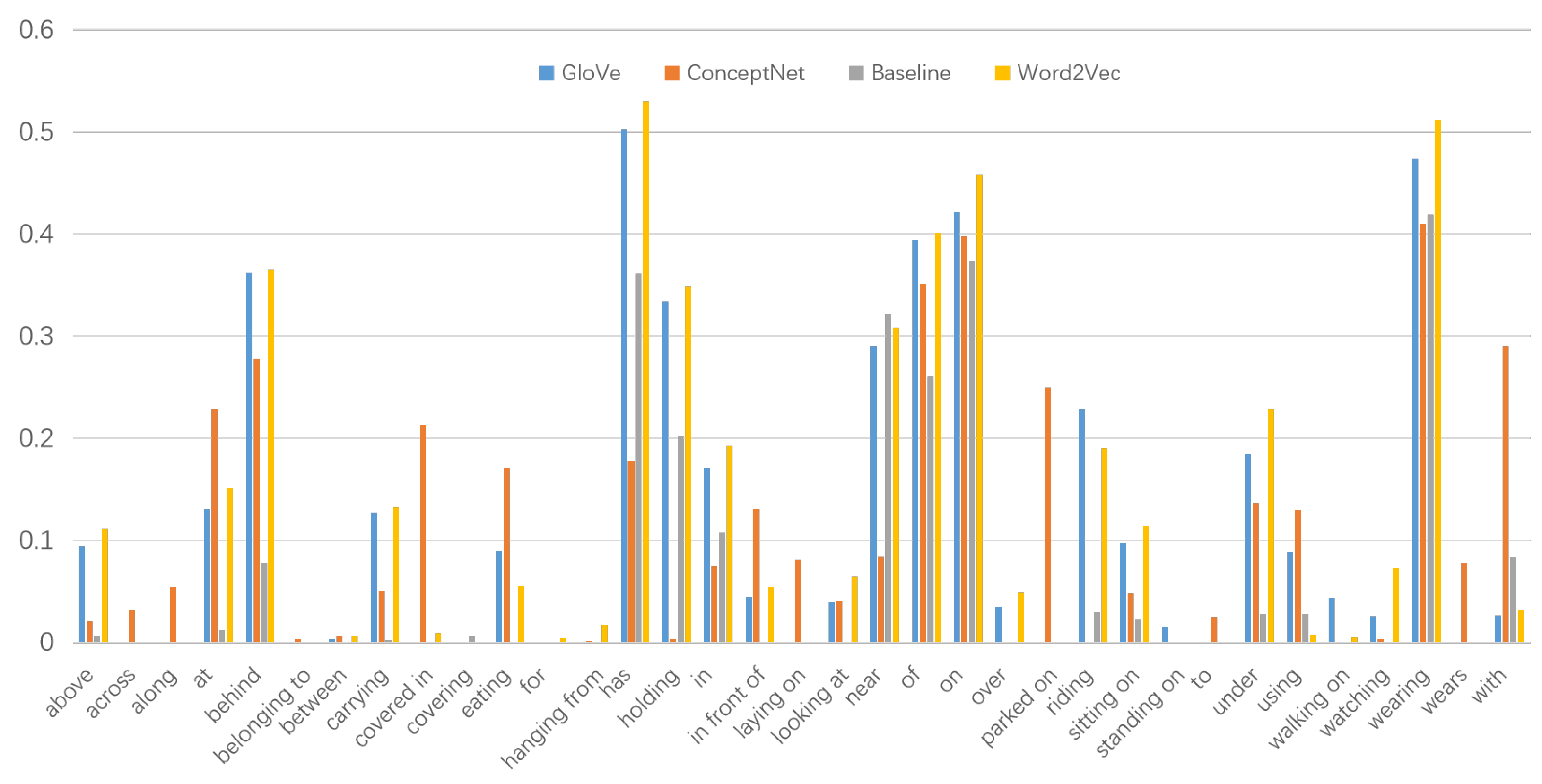
In terms of relationship prediction, Figure 6 and Table 6 show that the baseline model (which does not incorporate any external knowledge) exhibits poor performance in predicting semantic relationships (such as carrying, eating, looking at, walking on, and watching). This finding demonstrates that the semantic information provided by the external knowledge can assist in SGG tasks and improve the relationship prediction accuracy. Moreover, Table 6 shows that the contextual information fusion method proposed in this paper effectively fuses visual information with external knowledge, thereby providing richer visual–semantic contextual information for relational reasoning. Therefore, the introduction of external knowledge can effectively improve the quality of visual scene graphs for relationship prediction.
Influence of different types of external knowledge on the SGG model.Table 6 shows that there are disparities in the semantic information provided by the three types of vectors. ConceptNet vectors contain more semantic information than the other two types of word vectors, because ConceptNet and the other external knowledge representation methods have different constructions. The ConceptNet results are established by extracting common-sense information from semi-structured sentences. Although relationships such as “across”, “along”, and “to” contain a high degree of semantic information, other knowledge organization methods have difficulty learning the semantic common sense indicated by human annotations and instead represent this common-sense information in a format that can be understood by computers. Thus, ConceptNet performs well in these relationship categories.
Nevertheless, although ConceptNet shows better performance in predicting certain relationships, for the three SGG tasks considered in this work, ConceptNet still performs worse than the other models. The average value of the R@20, R@50, and R@100 metrics of the ConceptNet word vectors on the three tasks is 41.22%, while the corresponding values for the GloVe and Word2Vec vectors are 44.74% and 44.01%, respectively.
Due to the fact that ConceptNet is a large-scale knowledge graph method, it can supplement certain semantic information in SGG tasks; however, the rich semantic information contained in the entity vectors in the knowledge graph is more suitable for solving natural-language-reasoning problems than the semantic information provided by the ConceptNet vectors. Thus, for the relational reasoning task in the generation of visual scene graphs, better external knowledge organizations can be selected.
Table 4 shows that the GloVe performance on the three SGG tasks is slightly higher than the Word2Vec performance in terms of the R@K indicator. The reason for this result is that GloVe and Word2Vec have different knowledge organization approaches. In contrast to ConceptNet, which requires manual semi-structured common sense extraction and other operations during the initial stage, GloVe and Word2Vec allow computers to automatically generate word vectors from certain corpora based on specific algorithms.
4.4.2. Experiments on the Effects of the Visual Dependency
In this section, we use the method introduced in Section 3.3 to impose three constraints on the visual dependencies and explore the performance after these constraints are added in terms of the mR@K metric. In these approaches, the visual relationship dependencies (Vis), visual context dependencies (Ctx), or visual relationship and visual context dependencies (Vis+Ctx) are constrained. We introduce the mR@K indicator to comprehensively evaluate the performance of our SGG model after the visual dependency constraints are imposed. We assess the performance of the model in different prediction ranges by choosing K values of 20, 50, and 100. The results mainly explore the influence of the visual relationship characteristics and visual context characteristics on the visual dependency of the model. Future work will consider the influence of these characteristics on the visual dependency of the model for the particular case of small objects and their relationships.
Table 7 shows the mR@K () results for comparison. This table demonstrates that the Ctx model achieves the best performance in terms of all indicators on the PredCls, SGCls, and SGDet tasks. The results of the PredCls, SGCls, and SGDet tasks shown in Table 7 indicate that the method in which contextual dependencies (Ctx) are eliminated outperforms the other methods. According to these results, we present two ablation experiments in which we consider the influence of the visual relationships and context features on the visual dependency and the influence of the visual dependency constraints on the SGG model.
The Vis and Vis+Ctx models both perform worse than the B+G model; however, this finding does not indicate that applying the Vis or Vis+Ctx methods leads to poorer results. As shown in Table 8, compared with the B+G method, the Vis or Ctx methods increase the model’s ability to identify new relationships. When the zR@K metric is calculated, only triplets that do not appear in the training set are counted. Therefore, the Vis and Vis+Ctx methods increase the generalizability of the model by eliminating dependencies.
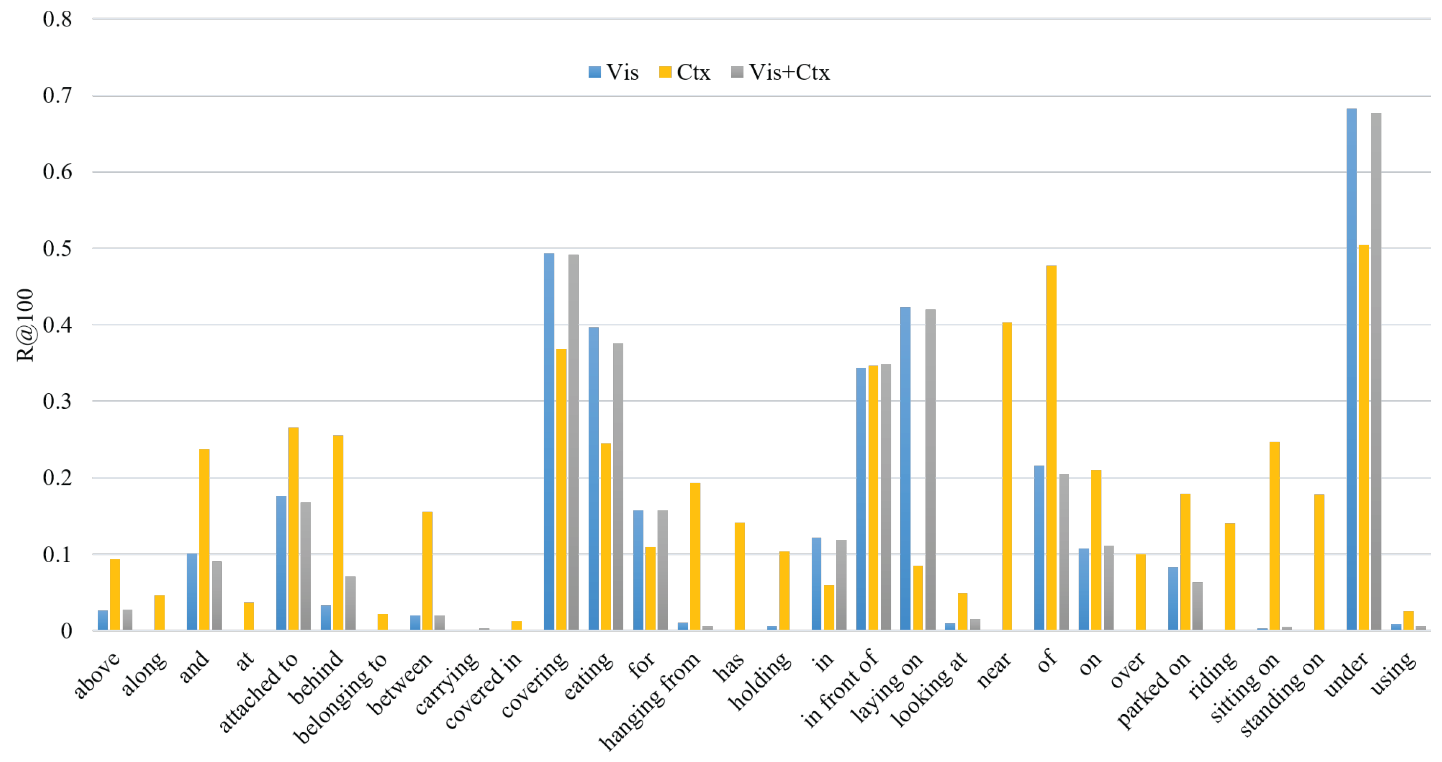
Influence of visual relationships and context features on the visual dependency. The SGDet task is used as an example to compare the R@100 values of each model to the test set for various relationships. The specific experimental results are shown in Figure 7 (the relationship categories for which the R@100 value of each model is 0 are omitted from the figure).
As shown in Table 7, the average mR@K value of the Vis method over the three tasks is 8.67%, the average mR@K value of the Vis+Ctx method is 8.61%, and the average mR@K value of the Ctx method is 13.32%. For the three SGG tasks, the model performance is optimal when the visual dependencies of the visual context features are eliminated. When the visual relationship features (the visual characteristics of the joint region of an object pair) and the visual dependencies of the visual relationship and visual context features are both removed, the model performs worse than the other methods.
Thus, according to our analysis, the model relies primarily on visual information for relational reasoning. If the visual information is removed during the learning process, the model relies only on the semantic information of the objects for relational reasoning and thus cannot generate significant visual representations. Therefore, the Vis and Vis+Ctx methods show worse performance than the Ctx method.
However, as shown in Figure 7 and Table 9, when the influence of the visual features is removed, the relationship category prediction performance improves. Thus, the removal of the visual feature information from the model can alleviate visual dependencies to some extent, especially when the dataset has a large amount of data for a given relationship category (on, has, wearing, holding, in, etc.). However, the model needs visual features for relationship reasoning; without visual features, visual representations of these relationships may be difficult to learn. Thus, although the addition of visual relationship features can alleviate certain visual dependency issues in the model, since the model mainly learns visual representations based on the image, the visual dependencies caused by these visual relationship features can be ignored.
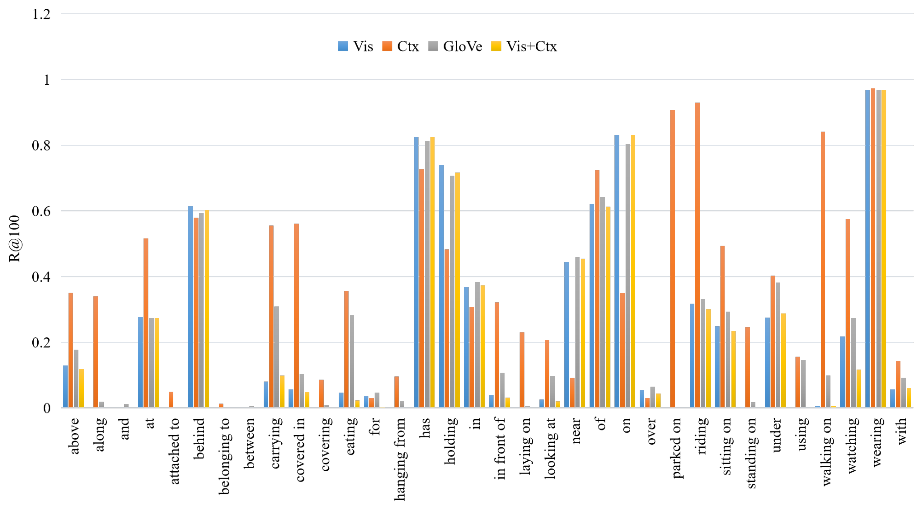
Furthermore, Figure 8 and Table 10 show that the visual dependency of the model is mainly due to the visual contextual information rather than the visual feature information. In the Ctx model, the visual context features can easily capture relationship categories that carry semantic information (such as along, covered in, hanging from, laying on, and parked on); thus, when the influence of these visual context features is removed from the model, the visual dependencies of the model can be alleviated.
Therefore, the above analysis demonstrates that, while the model exhibits visual dependencies based on both visual relationship features and visual context features, the most important information contained in the model is the visual relationship features rather than external knowledge or statistical information. Visual contextual information captures visual dependencies better than external knowledge or statistical information, because the visual context includes the spatial and semantic information of the targets. The model can determine object relationships based on this information; therefore, when the visual context features are removed from the model, the model directs more attention to the true visual relationships represented in the image rather than over-fitting based on the few relationship categories that account for the majority of the samples in the VG dataset.
In general, the experimental results shown in Table 9 and Table 10 demonstrate that the visual relationship features and visual context features both capture certain visual dependencies, especially the visual context features. To illustrate the performance of our method more clearly, Figure 9 shows some examples to compare the differences between the results of our method and the ground truth, demonstrating that our model identifies most objects and relationships.
5. Discussion
In summary, we introduce an SGG approach that uses external knowledge to successively update visual and contextual information and reduces visual dependencies by using the proposed visual context loss.
The semantic information contained in knowledge bases and visual dependencies is noisy; thus, our proposed module has the following design. First, the most relevant semantic information of a target instance is selected. Then, two BiLSTM encoders and a GRU decoder network are introduced to fuse the semantic and visual information in a successive manner. Finally, two loss functions are designed to learn the dependencies of the visual and semantic information. The proposed method is thoroughly explained, demonstrating the principles of the modules and the experimental results.
The ablation studies and experimental results demonstrate two key conclusions: (1) compared with other external knowledge bases, GloVe can better exploit the semantic information and is thus more suitable for our proposed model;and (2) although visual dependencies exist in both visual relationships (Vis) and semantic contexts (Ctx), the semantic context contains more visually dependent information. In addition, to further validate the superiority of the proposed model, we compared our model with previous models in terms of the R@K and mR@K metrics. The results show that our model outperforms the other models in most metrics.
However, some specific problems have yet to be solved. Our approach has two main limitations. First, the computational complexity of our methods is still high. In real visual scenes, most target pairs do not have relationships with each other, and considering all the relationships between targets in a scene introduces a considerable number of useless calculations, reducing the accuracy of the model. Second, due to the significant category imbalance in the dataset, the model over-fits large-sample relationships and may ignore small-sample relationships. Thus, although our proposed loss function reduces some of the visual dependence, the long-tail distribution problem is still present in the SGG task.
6. Conclusions and Future Work
In this work, we propose a knowledge-based SGG method with visual contextual dependencies. We apply two encoders to combine the visual features and external knowledge to determine the contextual information contained in a scene. Furthermore, two loss functions are designed to adjust the visual dependency of the model. As a result, we can generate more complete scene graphs than we could with previous methods. The experimental results indicate that the proposed model shows significant advantages over existing models in terms of the R@K and mR@K indicators. We believe that this study provides insight into the impact of different knowledge bases on the performance of scene graphs, as well as a new approach for handling visual dependencies.
In future work, we aim to reduce the computational complexity and visual dependence of our model to ensure that the model obtains unbiased features. First, we will design an efficient graphical structure to reduce the number of computations between pairs of invalid instances in the model. Second, we aim to explore unsupervised or weakly supervised methods to address the long-tail distribution problem. We believe that both approaches may improve the performance of our model. In addition, we hope to extend our model to scene graphs employed in other tasks, such as recommender systems and risky behaviour recognition.
Author Contributions
Conceptualization, L.Z. and H.Y.; Data curation, H.Y. and W.Z.; Investigation, S.L.; Methodology, L.Z. and H.Y.; Project administration, L.Z. and B.H.; Resources, L.Z., B.H. and S.L.; Software, H.Y. and W.Z.; Supervision, L.Z. and B.H.; Validation, H.Y.; Visualization, H.Y.; Writing—original draft, H.Y.; Writing—review & editing, L.Z. and H.Y. All authors have read and agreed to the published version of the manuscript.
Funding
This research work was partly supported by the Ministry of Science and Technology of Sichuan Province Program (2022YFG0038 and 2021YFG0018), and by the Fundamental Research Funds for the Central Universities (No. ZYGX2020ZB034 and No. ZYGX2021J019).
Institutional Review Board Statement
Not applicable.
Informed Consent Statement
Not applicable.
Data Availability Statement
The data presented in this study are available on request from the corresponding authors.
Conflicts of Interest
All authors certify that they have no affiliations with or involvement in any organization or entity with any financial interest or non-financial interest in the subject matter or materials discussed in this manuscript.
References
- Johnson, J.; Krishna, R.; Stark, M.; Li, L.J.; Shamma, D.; Bernstein, M.; Li, F.-F. Image retrieval using scene graphs. In Proceedings of the IEEE Conference on Computer Vision and Pattern Recognition, Long Beach, CA, USA, 15–20 June 2015; pp. 3668–3678. [Google Scholar]
- Fu, K.; Jin, J.; Cui, R.; Sha, F.; Zhang, C. Aligning where to see and what to tell: Image captioning with region-based attention and scene-specific contexts. IEEE Trans. Pattern Anal. Mach. Intell. 2016, 39, 2321–2334. [Google Scholar] [CrossRef] [PubMed]
- Zheng, X.; Cai, Z. Privacy-Preserved Data Sharing towards Multiple Parties in Industrial IoTs. IEEE J. Sel. Areas Commun. 2020, 38, 968–979. [Google Scholar] [CrossRef]
- Huang, L.; Wang, W.; Chen, J.; Wei, X.Y. Attention on attention for image captioning. In Proceedings of the IEEE/CVF International Conference on Computer Vision, Long Beach, CA, USA, 16–20 June 2019; pp. 4634–4643. [Google Scholar]
- Karpathy, A.; Li, F.-F. Deep visual–semantic alignments for generating image descriptions. In Proceedings of the IEEE Conference on Computer Vision and Pattern Recognition, Boston, MA, USA, 7–12 June 2015; pp. 3128–3137. [Google Scholar]
- Ramanathan, V.; Li, C.; Deng, J.; Han, W.; Li, Z.; Gu, K.; Li, F.-F. Learning semantic relationships for better action retrieval in images. In Proceedings of the IEEE Conference on Computer Vision and Pattern Recognition, Boston, MA, USA, 7–12 June 2015; pp. 1100–1109. [Google Scholar]
- Antol, S.; Agrawal, A.; Lu, J.; Mitchell, M.; Batra, D.; Zitnick, C.L.; Parikh, D. Vqa: Visual question answering. In Proceedings of the IEEE International Conference on Computer Vision, Santiago, Chile, 7–13 December 2015; pp. 2425–2433. [Google Scholar]
- Chang, A.; Savva, M.; Manning, C.D. Learning spatial knowledge for text to 3d scene generation. In Proceedings of the 2014 Conference on Empirical Methods in Natural Language Processing (EMNLP), Doha, Qatar, 25–29 October 2014; pp. 2028–2038. [Google Scholar]
- Cai, Z.; He, Z. Trading private range counting over big IoT data. In Proceedings of the 39th IEEE International Conference on Distributed Computing Systems (ICDCS 2019), Dallas, TX, USA, 7–9 July 2019. [Google Scholar]
- Singh, A.; Natarajan, V.; Shah, M.; Jiang, Y.; Chen, X.; Batra, D.; Parikh, D.; Rohrbach, M. Towards vqa models that can read. In Proceedings of the IEEE/CVF Conference on Computer Vision and Pattern Recognition, Long Beach, CA, USA, 15–20 June 2019; pp. 8317–8326. [Google Scholar]
- Teney, D.; Liu, L.; van DenHengel, A. Graph-structured representations for visual question answering. In Proceedings of the IEEE Conference on Computer Vision and Pattern Recognition, Honolulu, HI, USA, 21–26 July 2017; pp. 1–9. [Google Scholar]
- Tang, K.; Zhang, H.; Wu, B.; Luo, W.; Liu, W. Learning to compose dynamic tree structures for visual contexts. In Proceedings of the IEEE/CVF Conference on Computer Vision and Pattern Recognition, Long Beach, CA, USA, 16–17 June 2019; pp. 6619–6628. [Google Scholar]
- Dong, X.; Gan, T.; Song, X.; Wu, J.; Cheng, Y.; Nie, L. Stacked hybrid-attention and group collaborative learning for unbiased scene-graph generation. In Proceedings of the IEEE/CVF Conference on Computer Vision and Pattern Recognition, New Orleans, LA, USA, 21–24 June 2022; pp. 19427–19436. [Google Scholar]
- Xu, D.; Zhu, Y.; Choy, C.B.; Li, F.-F. Scene graph generation by iterative message passing. In Proceedings of the IEEE Conference on Computer Vision and Pattern Recognition, Honolulu, HI, USA, 21–26 July 2017; pp. 5410–5419. [Google Scholar]
- Zellers, R.; Yatskar, M.; Thomson, S.; Choi, Y. Neural motifs: Scene graph parsing with global context. In Proceedings of the IEEE Conference on Computer Vision and Pattern Recognition, Salt Lake City, UT, USA, 18–23 June 2018; pp. 5831–5840. [Google Scholar]
- Cai, Z.; Xiong, Z.; Xu, H.; Wang, P.; Li, W.; Pan, Y. Generative adversarial networks: A survey toward private and secure applications. ACM Comput. Surv. 2021, 54, 1–38. [Google Scholar] [CrossRef]
- Cai, Z.; Zheng, X. A private and efficient mechanism for data uploading in smart cyber-physical systems. IEEE Trans. Netw. Sci. Eng. (TNSE) 2020, 7, 766–775. [Google Scholar] [CrossRef]
- Cai, Z.; He, Z.; Guan, X.; Li, Y. Collective data-sanitization for preventing sensitive information inference attacks in social networks. IEEE Trans. Dependable Secur. Comput. 2018, 15, 577–590. [Google Scholar] [CrossRef]
- Chen, T.; Yu, W.; Chen, R.; Lin, L. Knowledge-embedded routing network for scene graph generation. In Proceedings of the IEEE/CVF Conference on Computer Vision and Pattern Recognition, Long Beach, CA, USA, 15–20 June 2019; pp. 6163–6171. [Google Scholar]
- Zareian, A.; Karaman, S.; Chang, S.F. Bridging knowledge graphs to generate scene graphs. In Proceedings of the European Conference on computer Vision, Glasgow, UK, 23–28 August 2020; Springer: Berlin/Heidelberg, Germany, 2020; pp. 606–623. [Google Scholar]
- Li, Y.; Ouyang, W.; Zhou, B.; Wang, K.; Wang, X. Scene graph generation from objects, phrases and region captions. In Proceedings of the IEEE International Conference on Computer Vision, Venice, Italy, 22–29 October 2017; pp. 1261–1270. [Google Scholar]
- Zhang, H.; Kyaw, Z.; Chang, S.; Chua, T. Visual translation embedding network for visual relation detection. In Proceedings of the IEEE Conference on Computer VISION and Pattern Recognition, Honolulu, HI, USA, 21–26 July 2017; pp. 5532–5540. [Google Scholar]
- Bordes, A.; Usunier, N.; Garcia-Duran, A.; Weston, J.; Yakhnenko, O. Translating embeddings for modeling multi-relational data. Adv. Neural Inf. Process. Syst. 2013, 26. [Google Scholar]
- Dai, B.; Zhang, Y.; Lin, D. Detecting visual relationships with deep relational networks. In Proceedings of the IEEE Conference on Computer Vision and Pattern Recognition, Honolulu, HI, USA, 21–26 July 2017; pp. 3076–3086. [Google Scholar]
- Newell, A.; Deng, J. Pixels to graphs by Associative Embedding. arXiv 2017, arXiv:170607365. [Google Scholar]
- Wang, W.; Wang, R.; Shan, S.; Chen, X. Sketching image gist: Human-mimetic hierarchical scene graph generation. In Proceedings of the European Conference on Computer Vision, Glasgow, UK, 23–28 August 2020; Springer: Berlin/Heidelberg, Germany, 2020; pp. 222–239. [Google Scholar]
- Li, Y.; Ouyang, W.; Zhou, B.; Shi, J.; Zhang, C.; Wang, X. Factorizable net: An efficient subgraph-based framework for scene graph generation. In Proceedings of the European Conference on Computer Vision (ECCV), Munich, Germany, 8–14 September 2018; pp. 335–351. [Google Scholar]
- Herzig, R.; Raboh, M.; Chechik, G.; Berant, J.; Globerson, A. Mapping images to scene graphs with permutation-invariant structured prediction. In Proceedings of the Advances Neural Information Processing Systems, Montreal, QC, Canada, 2–8 December 2018; p. 31. [Google Scholar]
- Woo, S.; Kim, D.; Cho, D.; Kweon, I.S. Linknet: Relational embedding for scene graph. In Proceedings of the Advances in Neural Information Processing Systems, Montreal, QC, Canada, 2–8 December 2018; p. 31. [Google Scholar]
- Zareian, A.; Karaman, S.; Chang, S. Weakly supervised visual semantic parsing. In Proceedings of the IEEE/CVF Conference on Computer Vision and Pattern Recognition, Munich, Germany, 8–14 September 2018; pp. 3736–3745. [Google Scholar]
- Gu, J.; Zhao, H.; Lin, Z.; Li, S.; Cai, J.; Ling, M. Scene graph generation with external knowledge and image reconstruction. In Proceedings of the IEEE/CVF Conference on Computer Vision and Pattern Recognition, Long Beach, CA, USA, 15–20 June 2019; pp. 1969–1978. [Google Scholar]
- Yang, J.; Lu, J.; Lee, S.; Batra, D.; Parikh, D. Graph r-cnn for scene-graph generation. In Proceedings of the European Conference on Computer Vision (ECCV), Munich, Germany, 8–14 September 2018; pp. 670–685. [Google Scholar]
- Qi, M.; Li, W.; Yang, Z.; Wang, Y.; Luo, J. Attentive relational networks for mapping images to scene graphs. In Proceedings of the IEEE/CVF Conference on Computer Vision and Pattern Recognition, Long Beach, CA, USA, 15–20 June 2019; pp. 3957–3966. [Google Scholar]
- Zhang, J.; Kevin, J.S.; Ahmed, E.; Tao, A.; Catanzaro, B. Graphical contrastive losses for scene graph parsing. In Proceedings of the IEEE/CVF Conference on Computer Vision and Pattern Recognition, Salt Lake City, UT, USA, 18–23 June 2019; pp. 11535–11543. [Google Scholar]
- Chen, L.; Zhang, H.; Xiao, J.; He, X.; Pu, S.; Chang, S. Counterfactual critic multi-agent training for scene graph generation. In Proceedings of the IEEE/CVF International Conference on Computer Vision, Rome, Italy, 19–21 October 2019; pp. 4613–4623. [Google Scholar]
- Mikolov, T.; Chen, K.; Corrado, G.; Dean, J. Efficient estimation of word representations in vector space. arXiv 2013, arXiv:13013781. [Google Scholar]
- Mikolov, T.; Sutskever, I.; Chen, K.; Corrado, G.S.; Dean, J. Distributed representations of words and phrases and their compositionality. In Proceedings of the Advances in Neural Information Processing Systems, Lake Tahoe, NV, USA, 5–8 December 2013; pp. 3111–3119. [Google Scholar]
- Pennington, J.; Socher, R.; Manning, C.D. Glove: Global vectors for word representation. In Proceedings of the 2014 Conference on Empirical Methods in Natural Language Processing (EMNLP), Doha, Qata, 25–29 October 2014; pp. 1532–1543. [Google Scholar]
- Speer, R.; Chin, J.; Havasi, C. Conceptnet 5.5: An open multilingual graph of general knowledge. In Proceedings of the Thirty-First AAAI Conference on Artificial Intelligence, San Francisco, CA, USA, 4–9 February 2017. [Google Scholar]
- Krishna, R.; Zhu, Y.; Groth, O.; Johnson, J.; Hata, K.; Kravitz, J.; Chen, S.; Kalantidis, Y.; Li, L.-J.; Shamma, D.A.; et al. Visual genome: Connecting language and vision using crowdsourced dense image annotations. Int. J. Comput. Vision 2017, 123, 32–73. [Google Scholar] [CrossRef] [Green Version]
- Lu, C.; Krishna, R.; Bernstein, M.; Li, F.-F. Visual relationship detection with language priors. In Proceedings of the European Conference on Computer Vision, Amsterdam, The Netherlands, 8–16 October 2016; Springer: Berlin/Heidelberg, Germany, 2016; pp. 852–869. [Google Scholar]
- Woo, S.; Noh, J.; Kim, K. Tackling the challenges in scene-graph generation with local-to-global interactions. IEEE Trans. Neural Netw. Learn. Syst. 2022. [Google Scholar] [CrossRef] [PubMed]
Figure 1.
(a) An example of an SGG model. (b) Different visual representations of similar relationships in the Visual Genome dataset. (c) An intuitive example of eliminating visual dependencies caused by external knowledge or visual information bias. It should be noted that the background blurring is applied only for illustration and should not be considered part of the visual processing step.

Figure 2.
Overview of our proposed modules. First, the feature-extraction module extracts visual features in the images. Then, the relational reasoning module combines external knowledge and visual features to obtain the global contextual information. Finally, the visual dependency constraint module reduces visual dependencies in the model.

Figure 3.
Structure of the feature extraction module.

Figure 4.
Structure of the relational reasoning module. GloVe word vectors are used to represent our external knowledge. GloVe uses the initial object class to determine the first word vector . Then, the word vector , object features, and bounding boxes are input into Encoder 1 to determine the visual–semantic context . After the first encoder, we decode to obtain an updated object class . GloVe then uses to obtain an updated word vector . Finally, and are input into the second encoder, yielding rich contextual information. The classifier predicts the relationships between object pairs based on the contextual information and the union features output by the feature-extraction module.

Figure 5.
(a) Example of applying the object features and word vectors to predict object relationships, where X represents the visual features of the objects of interest, W represents the corresponding word vector in the external knowledge base, and R represents the prediction. (b) The process of adjusting the visual dependencies. The objective of this process is to preserve valid information while minimizing unrelated information.

Figure 6.
Comparison of the R@100 values of different models for various relationships, calculated on the test set for the SGCls task. The X-axis represents the common relationship categories in the dataset, and the Y-axis represents the R@100 values.
Figure 6.
Comparison of the R@100 values of different models for various relationships, calculated on the test set for the SGCls task. The X-axis represents the common relationship categories in the dataset, and the Y-axis represents the R@100 values.

Figure 7.
Comparison of the R@100 values of different models on the test set for various types of relationships in the SGDet task. The X-axis represents the common relationship categories in the dataset, and the Y-axis represents the R@100 values.
Figure 7.
Comparison of the R@100 values of different models on the test set for various types of relationships in the SGDet task. The X-axis represents the common relationship categories in the dataset, and the Y-axis represents the R@100 values.

Figure 8.
Comparison of the R@100 values of different models on the test set for various types of relationships in the PredCls task. The X-axis represents the common relationship categories in the dataset, and the Y-axis represents the R@100 values.
Figure 8.
Comparison of the R@100 values of different models on the test set for various types of relationships in the PredCls task. The X-axis represents the common relationship categories in the dataset, and the Y-axis represents the R@100 values.

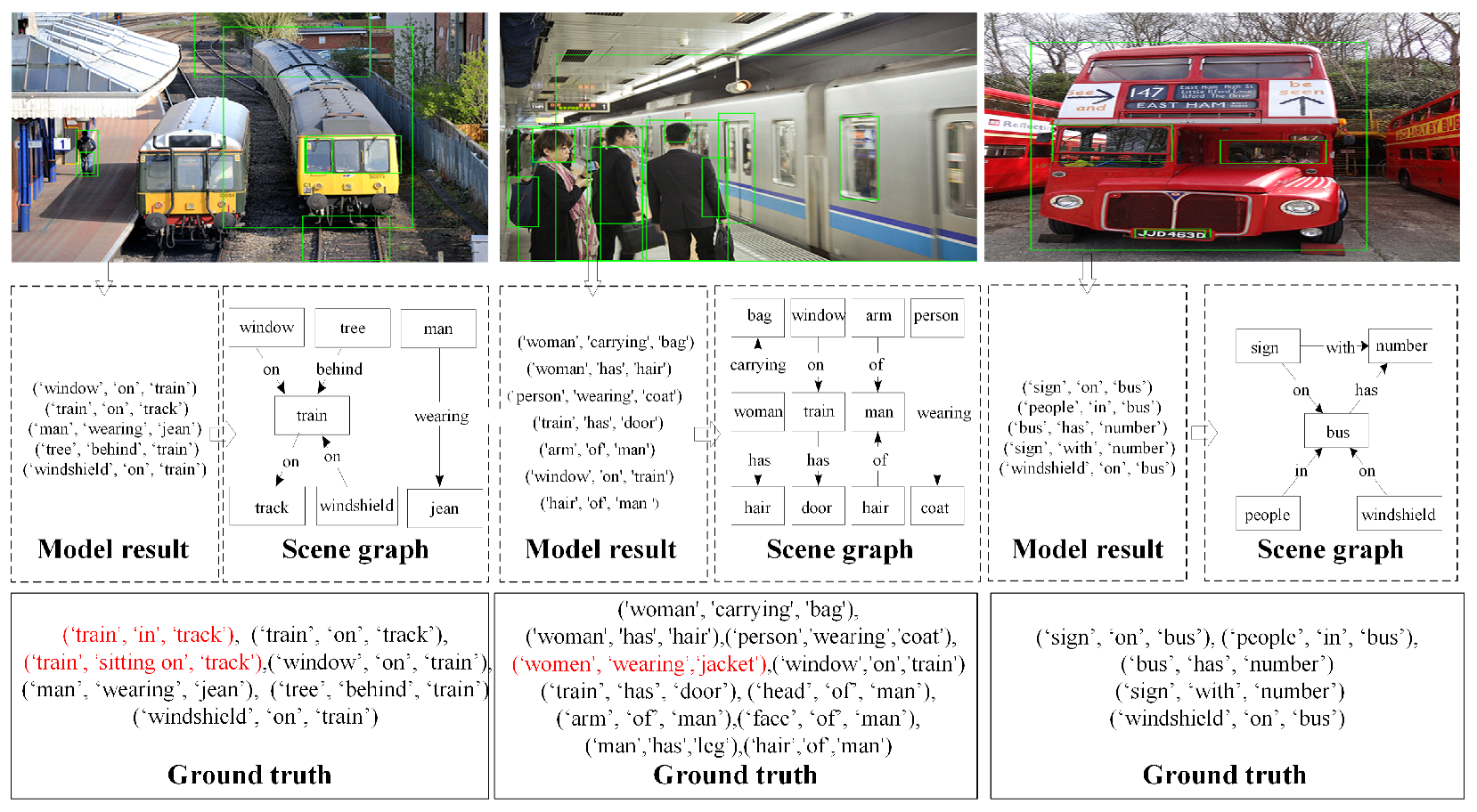
Figure 9.
Qualitative examples of the performance of our model. Our model can detect most of the relationships in the depicted scenes. (The red font indicates relationship triplets that were not found by our model).
Figure 9.
Qualitative examples of the performance of our model. Our model can detect most of the relationships in the depicted scenes. (The red font indicates relationship triplets that were not found by our model).


Table 1.
The parameters of experiments. (Kb represents the model of introducing external knowledge, Ctx represents the model of using visual contextual loss).
Table 1.
The parameters of experiments. (Kb represents the model of introducing external knowledge, Ctx represents the model of using visual contextual loss).
| Hyperparameter | Kb | Ctx |
|---|---|---|
| Batch size | 8 | 8 |
| Hidden dim | 512 | 512 |
| Learning rate | 0.008 | 0.006 |
| Weight decay | 0.0001 | 0.0001 |
| Dropout | [0.4, 0.2, 0.1] | [0.4, 0.3, 0.2] |
| Numbers of Iterations | [24,000, 24,000, 25,000] | [20,000, 28,000, 36,000] |
Table 2.
Comparison of the R@20, R@50, and R@100 metrics in % between our model and existing works. (Since the original paper lacks some results, the IMP+ results use the corresponding data presented in [15]).
Table 2.
Comparison of the R@20, R@50, and R@100 metrics in % between our model and existing works. (Since the original paper lacks some results, the IMP+ results use the corresponding data presented in [15]).
| PredCls | SGCls | SGDet | |||||||
|---|---|---|---|---|---|---|---|---|---|
| Model | R@20 | R@50 | R@100 | R@20 | R@50 | R@100 | R@20 | R@50 | R@100 |
| IMP+ [14,15] | \ | 59.3 | 61.3 | \ | 34.6 | 35.4 | \ | 20.7 | 24.5 |
| Motifs [15] | 58.5 | 65.2 | 67.1 | 32.9 | 35.8 | 36.5 | 21.4 | 27.2 | 30.3 |
| FREQ [15] | 53.6 | 60.6 | 62.2 | 29.3 | 32.3 | 32.9 | 20.1 | 26.2 | 30.1 |
| KERN [19] | \ | 65.8 | 67.6 | \ | 36.7 | 37.4 | \ | 27.1 | 29.8 |
| VCTree [12] | 60.1 | 66.4 | 68.1 | 35.2 | 38.1 | 38.8 | 22 | 27.9 | 31.3 |
| GB-NET [20] | \ | 66 | 68.2 | \ | 38 | 38.8 | \ | 26.4 | 30 |
| LOGIN [42] | 61.1 | 66.6 | 68.7 | 35.5 | 38.8 | 40.5 | 22.2 | 28.2 | 31.4 |
| Ours | 58.95 | 65.44 | 67.19 | 35.83 | 39.05 | 39.84 | 25.72 | 32.99 | 37.63 |
Table 3.
Comparison of the mR@20, mR@50, and mR@100 metrics in % between our model and existing works.
Table 3.
Comparison of the mR@20, mR@50, and mR@100 metrics in % between our model and existing works.
| PredCls | SGCls | SGDet | |||||||
|---|---|---|---|---|---|---|---|---|---|
| mR@20 | mR@50 | mR@100 | mR@20 | mR@50 | mR@100 | mR@20 | mR@50 | mR@100 | |
| IMP+ [14,15] | \ | 9.8 | 10.5 | \ | 5.8 | 6 | \ | 3.8 | 4.8 |
| Motifs [15] | 10.8 | 14 | 15.3 | 6.3 | 7.7 | 8.2 | 4.2 | 5.7 | 6.6 |
| FREQ [15] | 8.3 | 13 | 16 | 5.1 | 7.2 | 8.5 | 4.5 | 6.1 | 7.1 |
| KERN [19] | \ | 17.7 | 19.2 | \ | 9.4 | 10 | \ | 6.4 | 7.3 |
| VCTree [12] | 14 | 17.9 | 19.4 | 8.2 | 10.1 | 10.8 | 5.2 | 6.9 | 8 |
| GB-NET [20] | \ | 19.3 | 20.9 | \ | 9.6 | 10.2 | \ | 6.1 | 7.3 |
| LOGIN [42] | 16.0 | 19.2 | 22.3 | 8.6 | 11.2 | 12.4 | 5.9 | 7.7 | 9.1 |
| Ours | 15.23 | 21.66 | 25.35 | 8.02 | 11.05 | 12.8 | 6.42 | 8.78 | 10.58 |
Table 4.
Influence of different types of external knowledge on R@K.
| PredCls | SGCls | SGDet | Mean | |||||||
|---|---|---|---|---|---|---|---|---|---|---|
| R@20 | R@50 | R@100 | R@20 | R@50 | R@100 | R@20 | R@50 | R@100 | ||
| B | 58.77 | 65.37 | 67.12 | 25.38 | 28.36 | 29.33 | 25.34 | 32.35 | 37.52 | 41.06 |
| B+W | 58.83 | 65.40 | 67.17 | 35.53 | 38.73 | 39.55 | 25.55 | 32.48 | 32.87 | 44.01 |
| B+C | 59.02 | 65.50 | 67.27 | 25.88 | 28.33 | 28.96 | 25.70 | 32.96 | 37.37 | 41.22 |
| B+G | 58.95 | 65.44 | 67.19 | 35.83 | 39.05 | 39.84 | 25.72 | 32.99 | 37.63 | 44.74 |
Table 5.
Influence of different types of external knowledge on ngR@K.
| PredCls | SGCls | SGDet | Mean | |||||||
|---|---|---|---|---|---|---|---|---|---|---|
| ngR@20 | ngR@50 | ngR@100 | ngR@20 | ngR@50 | ngR@100 | ngR@20 | ngR@50 | ngR@100 | ||
| B | 67 | 81.51 | 88.63 | 28.6 | 34.95 | 38.34 | 27.01 | 36.23 | 43.32 | 49.51 |
| B+W | 67.07 | 81.55 | 88.73 | 40.6 | 48.21 | 51.77 | 27.2 | 36.82 | 43.65 | 53.96 |
| B+C | 67.21 | 81.67 | 88.69 | 30.83 | 37.76 | 41.62 | 27.33 | 36.99 | 43.81 | 50.66 |
| B+G | 67.2 | 81.72 | 88.8 | 40.93 | 48.66 | 52.21 | 27.3 | 36.93 | 43.69 | 54.18 |
Table 6.
R@100 values of each model for selected relationship categories in the SGCls task.
| Baseline | GloVe | ConceptNet | Word2Vec | |
|---|---|---|---|---|
| Model | R@100 | R@100 | R@100 | R@100 |
| Between | 0 | 0.35 | 0.69 | 0.69 |
| Eating | 0 | 8.94 | 17.09 | 5.52 |
| Looking at | 0 | 4.02 | 4.08 | 6.49 |
| Walking on | 0 | 4.43 | 0.13 | 0.54 |
| Watching | 0 | 2.55 | 0.38 | 7.26 |
Table 7.
Visual dependency reduction in terms of mR@K. Vis refers to applying , while Ctx refers to applying .
Table 7.
Visual dependency reduction in terms of mR@K. Vis refers to applying , while Ctx refers to applying .
| PredCls | SGCls | SGDet | Mean | |||||||
|---|---|---|---|---|---|---|---|---|---|---|
| mR@20 | mR@50 | mR@100 | mR@20 | mR@50 | mR@100 | mR@20 | mR@50 | mR@100 | ||
| B+G | 12.58 | 15.93 | 17.24 | 6.98 | 8.61 | 9.09 | 5.37 | 7.3 | 8.6 | 10.19 |
| Vis | 10.7 | 13.43 | 14.57 | 6.45 | 7.92 | 8.39 | 4.15 | 5.62 | 6.84 | 8.67 |
| Vis+Ctx | 10.44 | 13.05 | 14.11 | 6.59 | 8.19 | 8.68 | 4.12 | 5.52 | 6.76 | 8.61 |
| Ctx | 15.23 | 21.66 | 25.35 | 8.02 | 11.05 | 12.8 | 6.42 | 8.78 | 10.58 | 13.32 |
Table 8.
Visual dependency reduction in terms of zR@K.
| PredCls | SGCls | SGDet | Mean | |||||||
|---|---|---|---|---|---|---|---|---|---|---|
| zR@20 | zR@50 | zR@100 | zR@20 | zR@50 | zR@100 | zR@20 | zR@50 | zR@100 | ||
| B+G | 1.3 | 3.31 | 5.34 | 0.33 | 0.85 | 1.37 | 0.02 | 0.06 | 0.25 | 1.42 |
| Vis | 5.41 | 10.33 | 13.43 | 1.04 | 2.1 | 2.89 | 0 | 0.09 | 0.25 | 3.95 |
| Vis+Ctx | 5.3 | 10.29 | 13.7 | 1.17 | 2.04 | 2.97 | 0.02 | 0.04 | 0.28 | 3.98 |
| Ctx | 7.63 | 12.8 | 16.28 | 1.41 | 2.2 | 2.88 | 1.3 | 2.15 | 2.8 | 5.49 |
Table 9.
R@100 values of each model for selected relationship categories in the SGDet task.
| Vis | Ctx | Vis+Ctx | |
|---|---|---|---|
| On | 42.26 | 8.5 | 41.97 |
| Has | 49.37 | 36.84 | 49.14 |
| Wearing | 68.27 | 50.45 | 67.73 |
| Holding | 39.67 | 24.47 | 37.53 |
| In | 15.72 | 10.9 | 15.71 |
Table 10.
R@100 values of each model for selected relationship categories in the SGDet task.
| Vis | Ctx | Vis+Ctx | |
|---|---|---|---|
| Along | 0 | 4.59 | 0 |
| Covered in | 0 | 2.14 | 0 |
| Hanging from | 0 | 1.2 | 0 |
| Laying on | 0 | 14.17 | 0 |
| Parked on | 0 | 40.34 | 0 |
Publisher’s Note: MDPI stays neutral with regard to jurisdictional claims in published maps and institutional affiliations. |
© 2022 by the authors. Licensee MDPI, Basel, Switzerland. This article is an open access article distributed under the terms and conditions of the Creative Commons Attribution (CC BY) license (https://creativecommons.org/licenses/by/4.0/).
Share and Cite
MDPI and ACS Style
Zhang, L.; Yin, H.; Hui, B.; Liu, S.; Zhang, W. Knowledge-Based Scene Graph Generation with Visual Contextual Dependency. Mathematics 2022, 10, 2525. https://doi.org/10.3390/math10142525
AMA Style
Zhang L, Yin H, Hui B, Liu S, Zhang W. Knowledge-Based Scene Graph Generation with Visual Contextual Dependency. Mathematics. 2022; 10(14):2525. https://doi.org/10.3390/math10142525
Chicago/Turabian StyleZhang, Lizong, Haojun Yin, Bei Hui, Sijuan Liu, and Wei Zhang. 2022. "Knowledge-Based Scene Graph Generation with Visual Contextual Dependency" Mathematics 10, no. 14: 2525. https://doi.org/10.3390/math10142525
Note that from the first issue of 2016, this journal uses article numbers instead of page numbers. See further details here.