
An Evidential Software Risk Evaluation Model

1
College of Information and Engineering, Kunming University, Kunming 650214, China
2
Key Laboratory of Data Governance and Intelligent Decision, Universities of Yunnan, Kunming 650214, China
3
Institute of Fundamental and Frontier Science, University of Electronic Science and Technology of China, Chengdu 610054, China
*
Authors to whom correspondence should be addressed.
Mathematics 2022, 10(13), 2325; https://doi.org/10.3390/math10132325
Submission received: 9 April 2022
/
Revised: 19 June 2022
/
Accepted: 29 June 2022
/
Published: 2 July 2022
(This article belongs to the Special Issue Probability and Statistics in Quality and Reliability Engineering)
Abstract
:Software risk management is an important factor in ensuring software quality. Therefore, software risk assessment has become a significant and challenging research area. The aim of this study is to establish a data-driven software risk assessment model named DDERM. In the proposed model, experts’ risk assessments of probability and severity can be transformed into basic probability assignments (BPAs). Deng entropy was used to measure the uncertainty of the evaluation and to calculate the criteria weights given by experts. In addition, the adjusted BPAs were fused using the rules of Dempster–Shafer evidence theory (DST). Finally, a risk matrix was used to get the risk priority. A case application demonstrates the effectiveness of the proposed method. The proposed risk modeling framework is a novel approach that provides a rational assessment structure for imprecision in software risk and is applicable to solving similar risk management problems in other domains.
MSC:
90B251. Introduction
In today’s world, software is becoming more and more important in economy, healthcare, society, and other aspects of life [1,2,3]. In order to ensure the quality, reliability and stability of software, many methods have been proposed [4,5]. Software project risk management has become the focus of attention. A risk is an uncertain event or condition that may or may not occur. If it happens, the positive or negative impact effect on one or more objectives. Project teams endeavor to identify and evaluate known and emergent risks throughout the software life cycle. However, risk factors are so complex and uncertain that the effective identification and evaluation of them is still an open issue.
Most research has focused on risk analysis and risk management [6,7,8]. Different theories and techniques have been used to deal with risks. For example, a scheme to incorporate Bayesian belief networks in software project risk management presented by Fanv et al. [9]. Hu et al. [10] proposed a model using BNs with causality constraints for risk analysis of software development projects. Odzaly et al. [11] described the underlying risk management model in an Agile risk tool. An assessment model based on the combination of backpropagation neural network (BPNN) and rough set theory (RST) was put forward by Li et al. [12]. A computational model for the reduction of the probability of project failure through the prediction of risks was proposed by Filippetto et al. [13].
Among these methods, expert opinion and judgment are usually used to perform a risk assessment. One method of making statistical inferences and decisions based on expert opinion and judgment is expert knowledge elicitation. The related literature is extensive [14,15,16]. Since most experts prefer to express their opinions in a qualitative way, the expert elicitation procedure is full of subjectivity and uncertainty. It is important to provide a reliable framework for dealing with expert judgments [17]. Fuzzy set theory [18] is a common and accepted way of dealing with expert opinion and judgment. However, it has several flaws in expressing the hesitancy among several risk values. In some cases, due to a lack of experience or information, experts may not use a single risk level to describe their assessment, but rather hesitate between several risk values. For example, hesitation is between possible and very possible. The traditional fuzzy evaluation matrix cannot express the hesitation in the assessment. Furthermore, forming a fuzzy evaluation matrix takes a lot of time [19]. The fuzzy matrix needs to adjust assignment several times. The fuzzy matrix becomes more complex as the number of risk factors increases. Furthermore, it is not very efficient when dealing with complex fuzzy arithmetic operations. Therefore, it is necessary to propose a method that can efficiently represent multiple subsets without using matrices.
To solve these problems, a data-driven risk assessment model, based on Dempster–Shafer evidence theory (DST) [20,21], Deng entropy [22] and risk matrix [23], is proposed. Due to effectively deal with uncertain information, DST is widely used in decision-making [24,25,26], risk analysis [27], information fusion [28,29], uncertainty measurements [30], fault diagnosis [31,32,33], time-series [34], IoT applications [35] and many other fields [36,37]. Since most experts prefer to express their opinions with linguistic information, such as good, better, best, bad, worse, worst, DST can effectively deal with uncertain information about linguistic expressions involved in risk evaluation [38,39]. At the same time, it can also deal with the situation of multiple subsets due to the hesitation of experts. In some methods, the weights of experts or attributes are artificially assigned or not taken into account, which may lead to subjective results. Hence, expert assessments need to be adjusted reasonably. In the DST framework, Deng entropy is one of the most useful methods to measure uncertainty, and it has been applied in multi-sensor information fusion [40,41], decision-making [42,43], risk and reliability assessment [44] and other applications. The higher the Deng entropy, the more uncertainty there is. Therefore, in our proposed model, Deng entropy is used to measure the uncertain degree of assessments, and then obtain objective criteria weights given by experts. In addition, probability and severity are two critical descriptors of risk. As a convenient and efficient risk assessment tool, the risk matrix method has been widely used in the engineering field. It can be used to make a comprehensive assessment of probability and severity [45,46,47].
The main contributions of this paper are as follows:
- (1)
- Combining qualitative and quantitative factors at different scales. Various scales are used in the assessment, which are in line with real-world scenarios and help the experts to effectively express their opinion.
- (2)
- A method based on DST and Deng entropy is used for software risk assessment, which can adjust the expert assessment value and deal with the conflicting value in the assessment. This method makes the assessment more objective.
- (3)
- Development of a data-driven software risk evaluation model, which is an integration of DST, Deng entropy and risk matrix. The data can be converted into BPAs as soon as the experts give their evaluation values. After that, the BPAs are weighted and fused. Finally, risk rankings are obtained and provide information for risk decisions. It is effective not only in measuring uncertainty measures, but also in expert evaluation conflict handling and expert evaluation opinion integration.
This paper is structured as follows: In Section 2, basic definitions and operations of DST and Deng entropy are reviewed. In Section 3, the method of risk assessment framework is illustrated and the knowledge of software risk identification and risk assessment is introduced. An evidential model based on DST—the Deng entropy risk matrix—is proposed. In Section 4, a case application is shown. The results and discussion are presented in Section 5, and conclusions are drawn in Section 6.
2. Preliminaries
Dealing with uncertainty is still an open issue [48]. Various methods have been proposed, such as intuitionistic fuzzy values [49,50,51] and others [52]. These methods were applied in medical analysis, clustering, network congestion alleviating, search engine optimization techniques, etc. [53,54,55]. As an effective method for handling uncertainty, Dempster–Shafer evidence theory is well studied [56]. Some basic concepts and operations are presented in this section.
2.1. Dempster–Shafer Evidence Theory
Dempster–Shafer evidence theory (DST) was proposed by Dempster [20] and then expanded by Shafer [21]. The basic concepts are described below.
Definition 1.
Let Θ be a finite set with n exclusive and exhaustive elements, Θ = {}. The Θ is called the framework of identification (FOD). The power set of Θ consists of elements, which is denoted as,
Definition 2.
m is a mass function or a basic probability assignment (BPA), which satisfies , with the following constraints:
Definition 3.
For a proposition , the belief function is defined as,
The plausibility function Pl: is defined as,
[Bel(A), Pl(A)] is the belief interval of the proposition A.
Definition 4.
Conflict coefficient is k, which indicates the conflict degree between two BPAs. When means is consistent with , and when means totally contradicts , that is, the two pieces of evidence strongly support different hypotheses, and these hypotheses are incompatible [59].
Example 1.
Suppose Θ = {A, B}, two BPAs as follows,
2.2. Deng Entropy
Entropy is widely used in many fields, such as politics, economics, sociology, informatics, etc. There are many studies on entropy [60,61].
Definition 5.
Deng entropy is proposed in [22], which is a measure of uncertainty. Furthermore, it has been further improved in dealing with information volume [40,62]. It can be described as,
where m is a BPA defined on the FOD, and A is a focal element of m, is the cardinality of A.
Through a simple transformation, it can also be described as
Deng entropy is an improvement of Shannon entropy. The belief for each focal element in the Deng entropy is divided into . If there is no uncertainty, i.e., , the Deng entropy can degenerate to the Shannon entropy. Some properties and extension of Deng entropy are discussed in [63]. More research can be found in [64,65,66].
Example 2.
Suppose there is an expert evaluation, the frame of discernment is {A, B}. m(A) = 0.7, which represents the expert’s belief in A. The remaining belief is 0.3, representing the expert’s hesitation. The remaining belief is assigned to {A, B}, m(AB) = 0.3. The Deng entropy of the expert evaluation is calculated by Equation (7).
Example 3.
Suppose there is an expert evaluation, the frame of discernment is {A, B, C}. m(A) = 0.7, m(ABC) = 0.3. The Deng entropy of the expert evaluation is calculated by Equation (7).
From the above two examples, it can be seen that the value of the Deng entropy is related to the hesitation value of the experts in the evaluation. By using Deng entropy, the degree of uncertainty in evaluation information can be determined so that objective weights can be calculated. Therefore, it is a good method to apply Deng entropy in risk assessment.
3. Methodology
Some methods are introduced in this section. Software risk identification is shown in Section 3.1. Software risk assessment is explained in Section 3.2. An evidential software risk evaluation model DST—Deng entropy risk matrix (DDERM)—is illustrated in Section 3.3.
3.1. Software Risk Identification
Risk identification is the first step in risk management. With the development of technology and the improvement of project management methods, a number of methods have been proposed to identify risks, such as the Delphi method, expert judgment, graphical techniques, brainstorming and other methods. Several risks are discussed in the different studies, as shown in Table 1.
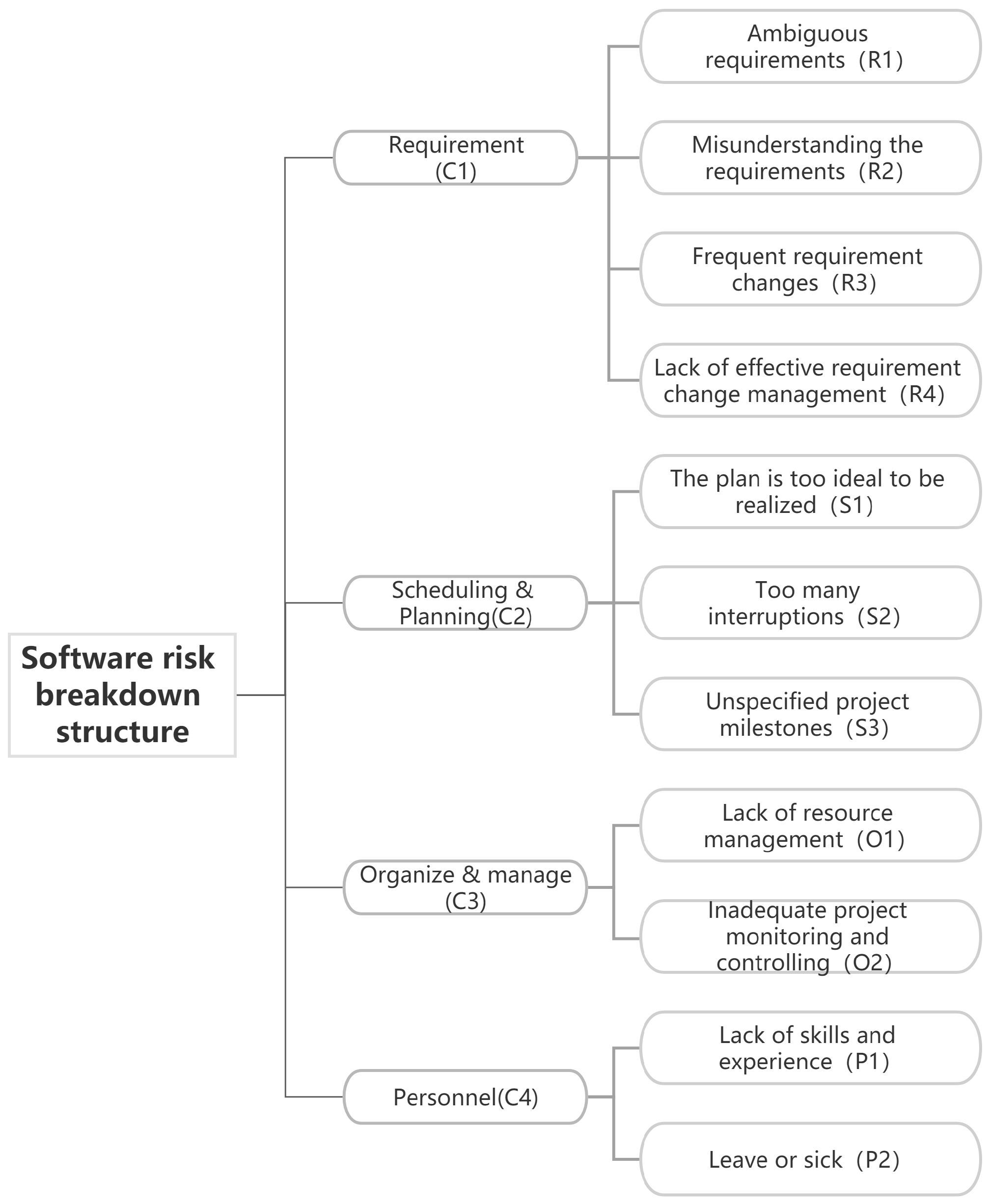
Risk factors always change with the environment. Meanwhile, different software projects have different risks. Based on the literature review discussed in Table 1, as well as on the previous experience of experts and analysis of the actual project situation, the DMs consider four types of risk factors in this project: requirement risks (C1), scheduling and planning risks (C2), organize and manage risks (C3) and personnel risks (C4). Details in Table 2. The software risk breakdown structure is shown in Figure 1. In the requirement risks (C1), there are four most common risks including ambiguous requirements (R1), misunderstanding the requirements risks (R2), frequent requirement changes (R3) and lack of effective requirement change management (R4). Scheduling and planning risks (C2) contains three risks: the plan is too ideal to be realized (S1), too many interruptions (S2), and unspecified project milestones (S3). Lack of resource management (O1) and inadequate project monitoring and controlling (O2) are in the organize and manage risks (C3). Lack of skills and experience (P1) and leave or sick (P2) are the most common personnel risks (C4).
Notably, some of these risk factors may not be independent. For example, lack of skills and experience (P1) may make it easier to misunderstand requirements (R2). However, the more risk factors there are, the more difficult it is to quantitatively measure the relationship between risk factors. Therefore, in the proposed model, the assessed values of the experts are considered to have taken into account the interrelationship between the risk factors.
3.2. Software Risk Assessment
Software risk assessment is to quantify the probability of risk and severity of loss, and then to obtain the overall level of system risk. The definition of risk can be shown as follows [74],
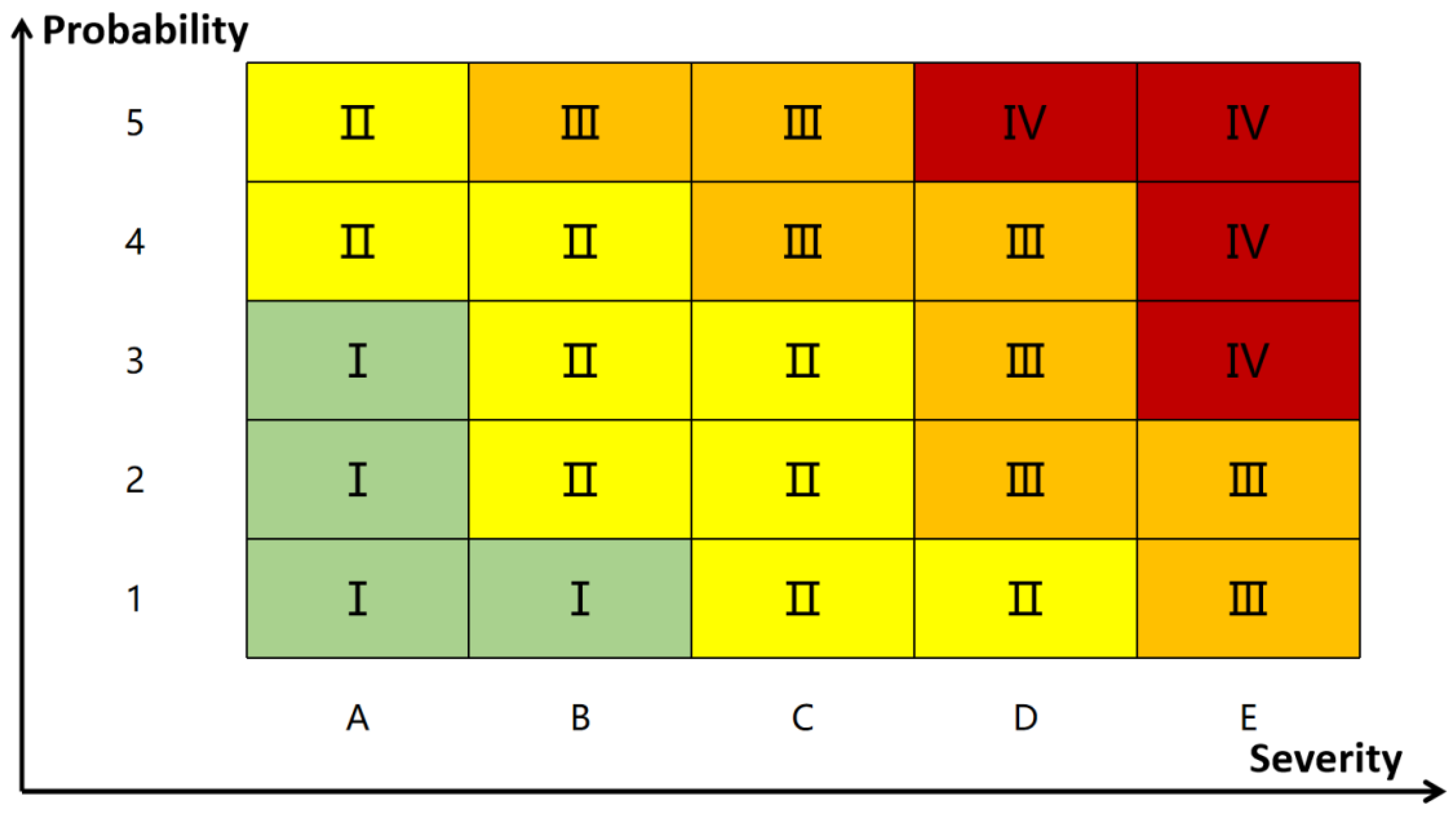
Probability and severity are two aspects of risk. The levels and linguistic terms for these two aspects are listed in Table 3 and Table 4. There are five levels of probability, from low to high: very unlikely, unlikely, even, possible and very possible. Severity also contains five levels: very little, little, medium, serious and catastrophic. There are four levels of risk, as shown in Table 5.
As a good risk management tool, risk matrix is widely used. According to Equation (9) and the values in Table 3, Table 4 and Table 5, a risk matrix is given in Table 6 and its levels are shown in Figure 2. If the severity of a risk is serious, but the probability of occurrence is very unlikely, the risk is still very low. Furthermore, if the probability is very possible, but the impact is little, the risk is medium. For example, the probability of risk R1 is level 4, and its severity is D. By querying the risk matrix, its risk level is III. Therefore, both factors must be taken into account to determine the risk level.
3.3. DST—Deng Entropy Risk Matrix Model
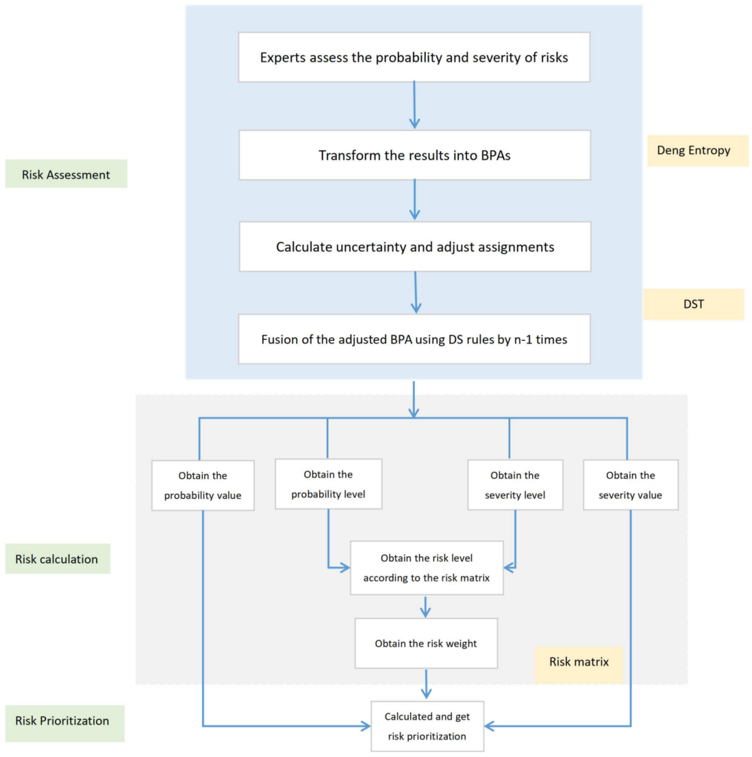
Good risk management is an important condition to ensure system reliability. For more research on reliability, please refer to [75,76]. A risk assessment model DST—Deng entropy risk matrix (DDERM) is proposed to deal with risk data. This model is composed of the following steps, as illustrated in Figure 3.
Step 1. Each expert makes judgments on each risk in the risk list, including both probability and severity;
Step 2. Transform the assessment results into BPAs;
Step 3. Calculate uncertainty and adjust assignments;
Step 3.1. Calculate the uncertainty.
where ℜ represents different risk factors, such as R1, R2, S1, O1, O2, P1, and so on. For each ℜ, there are n experts’ assigned values. is the assignment of the i-th expert. is the frame of discernment of probability, and = {1, 2, 3, 4, 5}. is the frame of discernment of severity, and = {A, B, C, D, E}.
Step 3.3. Modify each BPA.
Step 4. Fusion of the adjusted BPAs using DS rules. If there are n experts, n − 1 times of fusion are performed.
where k is conflicting factors.
Step 5. According to the result of fusion, the values of probability and severity can be obtained. Meanwhile, the level of probability and severity can also be obtained.
Step 6. According to the risk matrix in Figure 2, risk levels are obtained by using the probability level and the severity level.
Step 7. Get the weight of risk based on risk level, as shown in Table 7.
Step 8. Calculate and get risk prioritization.
4. A Case Application
This case is an application of software risk management. Software risk management is closely related to software quality. In recent years, the problem of poor quality software has occurred frequently, seriously affecting the production and lives of people. Therefore, it is necessary to establish an effective risk assessment model for better risk management.
As we know, effectively representing, aggregating and ranking risk factors should be the key issues in risk management. In the application, after risk identification, eleven risk factors are listed in Table 2. Three experts were invited to assess the risk. In order to represent the assessed values effectively, the assessed values are converted to BPAs. Meanwhile, Deng entropy and DST are used to aggregate risks. Finally, the risk matrix is used to calculate the risk ranking.
Step 1. For the eleven key factors in Table 2, three experts were invited to express their opinions on probability and severity according to the levels defined in Table 3 and Table 4. Here, we assume that the experts have the same knowledge weights. Evaluation are given in Table 8. For instance, the risk R1, 4 (80%) means that expert 1 is 80% sure that the probability of risk is “Possible.” Furthermore, D (60%) means that the severity of “Serious” is 60%, which is the estimate given by expert 1.
Step 2. Transform the assessment results into BPAs.
For risk P1, the BPAs of the probability are as follows,
The BPAs of the severity are as shown below,
Since , if the BPAs of a risk given by an expert is not equal to 1, assign the remaining value to .
Step 3. Calculate uncertainty and adjust assignments.
Step 3.1. Calculate the uncertainty. Still using P1 as an example, base on Equation (10) the uncertainty degree of probability is calculated as follows:
Base on Equation (11) the uncertainty degree of severity is .
In the same way, use Equation (13) to calculate other w of P1, .
In the same way, .
Step 4. Fusion of the adjusted BPAs using DS rules by n-1 times based on Equations (16) and (17). Because there are three sets of BPAs, it needs to fused two times.
Step 5. According to the result of fusion, the values of probability and severity can be obtained. Meanwhile, the probability and severity levels can also be obtained. The fuse results are presented in Table 9.
Step 6. According to the risk matrix, the probability level and the severity level can be used to obtain the risk level, as shown in Table 10.
Step 7. Get the weight of risk based on risk level, as shown in Table 7.
5. Results and Discussion
In this section, the results are analyzed. Furthermore, to demonstrate the advantages of the proposed method, a discussion is presented in the following.
5.1. Results
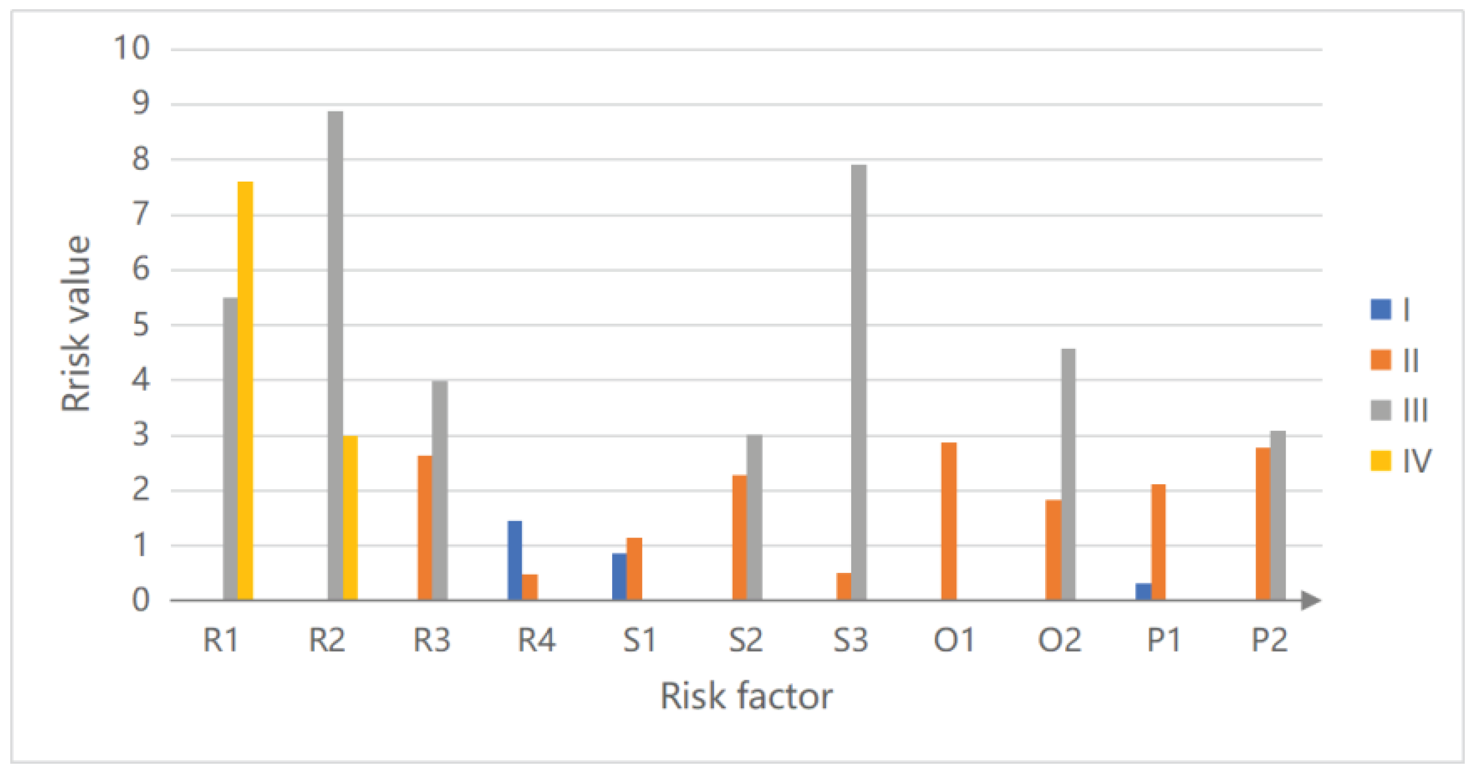
According to Table 11 and Figure 4, the results of the proposed risk assessment model DDERM can be seen from two perspectives.
For each risk factor, there may be different risk levels. For example, R1 contains two levels—one is III and the other is IV, while O1 has only one risk level II. The project manager and DM can consider whether to focus on high-level or low-level risk factors, according to the specific situation of the project, the nature of risks, different software life cycle periods, and risk preferences.
For each risk level, the risk factors can be sorted. In level I, R4 > S1 > P1. In level II, O1 > P2 > R3 > S4 > P1 > O2 > S1 > S3 > R4. R2 > S3 > R1 > O2 > R3 > P2 > S2 in level III. Furthermore, R1 > R2 in level IV. This means that, for the highest risk level ’High’, R1 must be focused first, and then R2. R2 is the most important in level ’Significant’. For the risk level ’Medium’, O1 is the most concerned. In ’Low’, R4 needs the most attention. The project manager and DMs can make decisions based on different risk levels.
Based on the results, some explanations are needed. R4 > P1 means “lack of effective requirement change management” presents a higher risk than “lack of skills and experience”. This may be because requirements changes occur frequently, and in this case, there is a significant risk if requirements changes are not managed effectively. At the same time, the members of this project team are all experienced in development, in comparison, the risk of” lack of skills and experience”is less. In addition, R1 > R2, which means that ambiguous requirements are more risky than misunderstood requirements. The result seems unreasonable. However, in this case, the possibility for the requirements analysis to completely misunderstand the requirements may be less than the user’s ambiguity in expressing the requirements, so R1 > R2. The assessed values of the experts are considered to have taken into account the interrelationship between the risk factors.
5.2. Compared with Other Software Risk Assessment Method
In this section, we compare the constructed DDERM model with several existing methods, including Fuzzy set theory and hierarchical structure [68,77], Fuzzy DEMATEL, FMCDM, TODIM approaches [69], DEMATEL, ANFIS MCDM and F-TODIM approaches [70], entropy-based method [67]. The comparison are shown in Table 12. We can draw the following conclusions:
- (1)
- In [68,77], the weights are given in advance. Thus, weights are static and subjective. In contrast, in the DDERM approach, the weights are measured by the degree of uncertainty in the assessment. The weights are objective and independent, and relate only to the assessment of risk factors. When different experts give different values for the same risk factor, the weights are definitely different. If the same expert evaluates different risks differently, the weights must be distinct. This means that the weight is dependent on how reliable the expert is for that risk. Besides, the evaluations of different experts have no effect on the weights of other experts.
- (2)
- In [69,70], multiple modifications to the judgment matrix are frequently required because the judgment matrix created during the evaluation process is not completely consistent. The judgment matrix needs to be modified more than 4 times. In the DDERM approach, there is no need to establish and repeatedly adjust the matrix. Only expert evaluation and risk matrix are required. At the same time, DDERM has the advantage of DST in expressing uncertain information, which effectively assigns risk value to multi subsets.
- (3)
- Using entropy-based method for software risk assessment in [67]. However, it does not effectively solve the problem of conflicting information in the assessment. Similarly, it is well know that Dempster’s combination rule is very important for multi-source combination. However, when fusing the high conflicting evidences, counter-intuitive conditions often occur. For example, suppose there are two options A and B. There are ten experts in total. 1 expert is very sure that it is A (assuming BPA is 0.99). 9 experts choose B, but the BPA is not very high (assuming the BPA is 0.6 each). The choice is A after using the Dempster’s combination rule. However, obviously, we are more certain that the choice of 9 experts is correct. In DDERM method, based on the Deng entropy, the higher the entropy value gives higher weight, which can effectively solve the drawbacks of Dempster’s combination rule about conflicts. In the example above, using this approach effectively downplays the impact of individual expert errors on the overall assessment.

Table 12.
Comparison of different method of software risk assessment.
| Literature | Processing Method | Calculation of Weights | Complexity | Subjective/ Objectivity |
|---|---|---|---|---|
| [68,77] | Fuzzy set theory and hierarchical structure analysis | Given in advance | Convert the linguistic value to triangular fuzzy number and multiply the fuzzy numbers | Weights are static and relatively subjective |
| [69,70] | Fuzzy DEMATEL + FMCDM + TODIM/DEMATEL + ANFIS MCDM + IF-TODIM | Fuzzy DEMATEL + Fuzzy TODIM | Multiple adjustments fuzzy matrix | Using integrated fuzzy approaches, assessment results are relatively objective |
| [67] | Entropy | Entropy weight method | Simple calculation | Uncertainty is taken into account and relatively objective |
| Our method | DST+Deng entropy+Risk Matrix | Deng entropy | Using data-driven model that does not need to calculate and adjust parameters many times | Considers uncertainty and conflicts between experts, more objectivity |
6. Conclusions
The evaluation of software risks plays an important role in the field of software development. To efficiently assess the risk, in this paper, a data-driven software risk evaluation model is proposed. We first discussed the drawbacks of the existing methods. Then, 11 software risks were identified. The software risk breakdown structure and risk matrix were illustrated. Furthermore, an evidential software risk evaluation model based on DST, Deng entropy and risk matrix were proposed. Finally, we applied the proposed method to a case application and compared our results to existing methods. By comparison, the proposed method can express more uncertainties and help the domain experts to express their opinions effectively. Meanwhile, it can adjust the expert assessment value and deal with the conflicting values in the assessment. In short, our method not only overcomes the complexity of matrix method, but also improves the ability to handle uncertainty. However, some limitations are also highlighted. More software risk factors would increase the validity of the results, and multiple weights were not considered. The evaluation process needs to be repeated when the risk factors change, since risk assessment is a dynamic process that exists throughout the life cycle of software.
Our future research work will mainly focus on considering the weight of risk attributes, giving experts different knowledge weights and improving the model to increase its applicability.
Author Contributions
Formal analysis, X.C. and Y.D.; Methodology, Y.D.; Writing—original draft, X.C.; Writing—review & editing, X.C. All authors have read and agreed to the published version of the manuscript.
Funding
The work is partially supported by National Natural Science Foundation of China (Grant No. 61973332), JSPS Invitational Fellowships for Research in Japan (Short-term).
Institutional Review Board Statement
Not applicable.
Informed Consent Statement
Not applicable.
Data Availability Statement
Not applicable.
Conflicts of Interest
The authors declare no conflict of interest. The funders had no role in the design of the study; in the collection, analyses, or interpretation of data; in the writing of the manuscript, or in the decision to publish the results.
References
- Fedushko, S.; Ustyianovych, T. Medical card data imputation and patient psychological and behavioral profile construction. Procedia Comput. Sci. 2019, 160, 354–361. [Google Scholar] [CrossRef]
- Pawade, D.; Pawade, Y.R.; Velankar, A.; Patel, R.K.; Mantri, Y. RAY: An App for Determining Decision-Making Power of a Person. I-Manag. J. Mob. Appl. Technol. 2016, 3, 33. [Google Scholar]
- Fedushko, S.; Ustyianovych, T. Operational Intelligence Software Concepts for Continuous Healthcare Monitoring and Consolidated Data Storage Ecosystem. In Proceedings of the International Conference on Computer Science, Engineering and Education Applications, Kiev, Ukraine, 21–22 January 2020; Springer: Berlin/Heidelberg, Germany, 2020; pp. 545–557. [Google Scholar]
- Triantafyllou, I.S.; Koutras, M.V. Reliability Properties of (n, f, k) Systems. IEEE Trans. Reliab. 2014, 63, 357–366. [Google Scholar] [CrossRef]
- Triantafyllou, I.S. On the Consecutive k1 and k2-out-of-n Reliability Systems. Mathematics 2020, 8, 630. [Google Scholar] [CrossRef] [Green Version]
- Boehm, B. Software risk management. In Proceedings of the European Software Engineering Conference, University of Warwick, Coventry, UK, 11–15 September 1989; Springer: Berlin/Heidelberg, Germany, 1989; pp. 1–19. [Google Scholar]
- Verdon, D.; McGraw, G. Risk analysis in software design. IEEE Secur. Priv. 2004, 2, 79–84. [Google Scholar] [CrossRef]
- Hu, Y.; Du, J.; Zhang, X.; Hao, X.; Ngai, E.; Fan, M.; Liu, M. An integrative framework for intelligent software project risk planning. Decis. Support Syst. 2013, 55, 927–937. [Google Scholar] [CrossRef]
- Fan, C.F.; Yu, Y.C. BBN-based software project risk management. J. Syst. Softw. 2004, 73, 193–203. [Google Scholar] [CrossRef]
- Hu, Y.; Zhang, X.; Ngai, E.; Cai, R.; Liu, M. Software project risk analysis using Bayesian networks with causality constraints. Decis. Support Syst. 2013, 56, 439–449. [Google Scholar] [CrossRef]
- Odzaly, E.E.; Greer, D.; Stewart, D. Agile risk management using software agents. J. Ambient Intell. Humaniz. Comput. 2018, 9, 823–841. [Google Scholar] [CrossRef] [Green Version]
- Li, X.; Jiang, Q.; Hsu, M.K.; Chen, Q. Support or risk? Software project risk assessment model based on rough set theory and backpropagation neural network. Sustainability 2019, 11, 4513. [Google Scholar] [CrossRef] [Green Version]
- Filippetto, A.S.; Lima, R.; Barbosa, J.L.V. A risk prediction model for software project management based on similarity analysis of context histories. Inf. Softw. Technol. 2021, 131, 106497. [Google Scholar] [CrossRef]
- Authority, E.F.S. Guidance on expert knowledge elicitation in food and feed safety risk assessment. EFSA J. 2014, 12, 3734. [Google Scholar]
- Bolger, F. The selection of experts for (probabilistic) expert knowledge elicitation. In Elicitation; Springer: Berlin/Heidelberg, Germany, 2018; pp. 393–443. [Google Scholar]
- O’Hagan, A. Expert knowledge elicitation: Subjective but scientific. Am. Stat. 2019, 73, 69–81. [Google Scholar] [CrossRef] [Green Version]
- Yazdi, M.; Zarei, E. Step Forward on How to Treat Linguistic Terms in Judgment in Failure Probability Estimation. In Linguistic Methods Under Fuzzy Information in System Safety and Reliability Analysis; Springer: Berlin/Heidelberg, Germany, 2022; pp. 193–200. [Google Scholar]
- Zadeh, L.A. Fuzzy sets. In Fuzzy Sets, Fuzzy Logic, and Fuzzy Systems: Selected Papers by Lotfi a Zadeh; World Scientific: Singapore, 1996; pp. 394–432. [Google Scholar]
- Xiao, F. CaFtR: A Fuzzy Complex Event Processing Method. Int. J. Fuzzy Syst. 2021, 24, 1098–1111. [Google Scholar] [CrossRef]
- Dempster, A.P. Upper and lower probabilities induced by a multivalued mapping. In Classic Works of the Dempster-Shafer Theory of Belief Functions; Springer: Berlin/Heidelberg, Germany, 2008; pp. 57–72. [Google Scholar]
- Shafer, G. A Mathematical Theory of Evidence; Princeton University Press: Princeton, NJ, USA, 1976. [Google Scholar]
- Deng, Y. Deng entropy. Chaos Solitons Fractals 2016, 91, 549–553. [Google Scholar] [CrossRef]
- Garvey, P.R.; Lansdowne, Z.F. Risk matrix: An approach for identifying, assessing, and ranking program risks. Air Force J. Logist. 1998, 22, 18–21. [Google Scholar]
- Song, Y.; Fu, Q.; Wang, Y.F.; Wang, X. Divergence-based cross entropy and uncertainty measures of Atanassov’s intuitionistic fuzzy sets with their application in decision making. Appl. Soft Comput. 2019, 84, 105703. [Google Scholar] [CrossRef]
- Song, M.; Sun, C.; Cai, D.; Hong, S.; Li, H. Classifying vaguely labeled data based on evidential fusion. Inf. Sci. 2022, 583, 159–173. [Google Scholar] [CrossRef]
- Khalaj, M.; Khalaj, F. An improvement decision-making method by similarity and belief function theory. In Communications in Statistics-Theory and Methods; Taylor & Francis: Abingdon, UK, 2021; pp. 1–19. [Google Scholar]
- Zhang, L.; Wang, Y.; Wu, X. Cluster-based information fusion for probabilistic risk analysis in complex projects under uncertainty. Appl. Soft Comput. 2021, 104, 107189. [Google Scholar] [CrossRef]
- Li, Y.; Deng, Y. Generalized Ordered Propositions Fusion Based on Belief Entropy. Int. J. Comput. Commun. Control 2018, 13, 792–807. [Google Scholar] [CrossRef]
- Su, X.; Li, L.; Shi, F.; Qian, H. Research on the fusion of dependent evidence based on mutual information. IEEE Access 2018, 6, 71839–71845. [Google Scholar] [CrossRef]
- Moral-García, S.; Abellán, J. Required mathematical properties and behaviors of uncertainty measures on belief intervals. Int. J. Intell. Syst. 2021, 36. [Google Scholar] [CrossRef]
- Ghosh, N.; Saha, S.; Paul, R. iDCR: Improved Dempster Combination Rule for multisensor fault diagnosis. Eng. Appl. Artif. Intell. 2021, 104, 104369. [Google Scholar] [CrossRef]
- Wang, T.; Liu, W.; Cabrera, L.V.; Wang, P.; Wei, X.; Zang, T. A novel fault diagnosis method of smart grids based on memory spiking neural P systems considering measurement tampering attacks. Inf. Sci. 2022, 596, 520–536. [Google Scholar] [CrossRef]
- Fan, J.; Qi, Y.; Liu, L.; Gao, X.; Li, Y. Application of an information fusion scheme for rolling element bearing fault diagnosis. Meas. Sci. Technol. 2021, 32, 075013. [Google Scholar] [CrossRef]
- Song, X.; Xiao, F. Combining time-series evidence: A complex network model based on a visibility graph and belief entropy. In Applied Intelligence; Springer: Berlin/Heidelberg, Germany, 2022. [Google Scholar] [CrossRef]
- Bezerra, E.D.C.; Teles, A.S.; Coutinho, L.R.; da Silva e Silva, F.J. Dempster–Shafer Theory for Modeling and Treating Uncertainty in IoT Applications Based on Complex Event Processing. Sensors 2021, 21, 1863. [Google Scholar] [CrossRef]
- Elmore, P.A.; Petry, F.E.; Yager, R.R. Dempster–Shafer approach to temporal uncertainty. IEEE Trans. Emerg. Top. Comput. Intell. 2017, 1, 316–325. [Google Scholar] [CrossRef]
- Deng, Y. Random Permutation Set. Int. J. Comput. Commun. Control 2022, 17, 4542. [Google Scholar] [CrossRef]
- Shams, G.; Hatefi, S.M.; Nemati, S. A Dempster-Shafer evidence theory for environmental risk assessment in failure modes and effects analysis of Oil and Gas Exploitation Plant. Sci. Iran. 2022. [Google Scholar] [CrossRef]
- Hatefi, S.M.; Basiri, M.E.; Tamošaitienė, J. An evidential model for environmental risk assessment in projects using dempster–shafer theory of evidence. Sustainability 2019, 11, 6329. [Google Scholar] [CrossRef] [Green Version]
- Deng, Y. Information Volume of Mass Function. Int. J. Comput. Commun. Control 2020, 15, 3983. [Google Scholar] [CrossRef]
- Xiao, F. An improved method for combining conflicting evidences based on the similarity measure and belief function entropy. Int. J. Fuzzy Syst. 2018, 20, 1256–1266. [Google Scholar] [CrossRef]
- Xiong, L.; Su, X.; Qian, H. Conflicting evidence combination from the perspective of networks. Inf. Sci. 2021, 580, 408–418. [Google Scholar] [CrossRef]
- Chen, L.; Li, Z.; Deng, X. Emergency alternative evaluation under group decision makers: A new method based on entropy weight and DEMATEL. Int. J. Syst. Sci. 2020, 51, 570–583. [Google Scholar] [CrossRef]
- Gao, X.; Su, X.; Qian, H.; Pan, X. Dependence assessment in Human Reliability Analysis under uncertain and dynamic situations. In Nuclear Engineering and Technology; Elsevier: Amsterdam, The Netherlands, 2021. [Google Scholar] [CrossRef]
- Ni, H.; Chen, A.; Chen, N. Some extensions on risk matrix approach. Saf. Sci. 2010, 48, 1269–1278. [Google Scholar] [CrossRef]
- Ruan, X.; Yin, Z.; Frangopol, D.M. Risk matrix integrating risk attitudes based on utility theory. Risk Anal. 2015, 35, 1437–1447. [Google Scholar] [CrossRef]
- Jianxing, Y.; Haicheng, C.; Shibo, W.; Haizhao, F. A novel risk matrix approach based on cloud model for risk assessment under uncertainty. IEEE Access 2021, 9, 27884–27896. [Google Scholar] [CrossRef]
- Wen, T.; Cheong, K.H. The fractal dimension of complex networks: A review. Inf. Fusion 2021, 73, 87–102. [Google Scholar] [CrossRef]
- Xie, D.; Xiao, F.; Pedrycz, W. Information Quality for Intuitionistic Fuzzy Values with Its Application in Decision Making. In Engineering Applications of Artificial Intelligence; Elsevier: Amsterdam, The Netherlands, 2021. [Google Scholar]
- Wang, Z.; Xiao, F.; Ding, W. Interval-valued intuitionistic fuzzy Jenson-Shannon divergence and its application in multi-attribute decision making. In Applied Intelligence; Springer: Berlin/Heidelberg, Germany, 2022. [Google Scholar] [CrossRef]
- Xiao, F. A distance measure for intuitionistic fuzzy sets and its application to pattern classification problems. IEEE Trans. Syst. Man Cybern. Syst. 2021, 51, 3980–3992. [Google Scholar] [CrossRef]
- Babajanyan, S.; Allahverdyan, A.; Cheong, K.H. Energy and entropy: Path from game theory to statistical mechanics. Phys. Rev. Res. 2020, 2, 043055. [Google Scholar] [CrossRef]
- Cheong, K.H.; Koh, J.M.; Jones, M.C. Paradoxical survival: Examining the parrondo effect across biology. BioEssays 2019, 41, 1900027. [Google Scholar] [CrossRef] [PubMed]
- Pawade, D.Y. Analyzing the Impact of Search Engine Optimization Techniques on Web Development Using Experiential and Collaborative Learning Techniques. Int. J. Mod. Educ. Comput. Sci. 2021, 2, 1–10. [Google Scholar] [CrossRef]
- Wang, H.; Fang, Y.P.; Zio, E. Resilience-oriented optimal post-disruption reconfiguration for coupled traffic-power systems. Reliab. Eng. Syst. Saf. 2022, 222, 108408. [Google Scholar] [CrossRef]
- Khalaj, F.; Khalaj, M. Developed cosine similarity measure on belief function theory: An application in medical diagnosis. In Communications in Statistics-Theory and Methods; Taylor & Francis: Abingdon, UK, 2020; pp. 1–12. [Google Scholar]
- Xiao, F. CEQD: A complex mass function to predict interference effects. IEEE Trans. Cybern. 2021. [Google Scholar] [CrossRef]
- Yan, Z.; Zhao, H.; Mei, X. An improved conflicting-evidence combination method based on the redistribution of the basic probability assignment. In Applied Intelligence; Springer: Berlin/Heidelberg, Germany, 2021; pp. 1–27. [Google Scholar]
- Cheng, C.; Xiao, F. A distance for belief functions of orderable set. Pattern Recognit. Lett. 2021, 145, 165–170. [Google Scholar] [CrossRef]
- Cui, H.; Zhou, L.; Li, Y.; Kang, B. Belief entropy-of-entropy and its application in the cardiac interbeat interval time series analysis. Chaos Solitons Fractals 2022, 155, 111736. [Google Scholar] [CrossRef]
- Khalaj, M.; Tavakkoli-Moghaddam, R.; Khalaj, F.; Siadat, A. New definition of the cross entropy based on the Dempster-Shafer theory and its application in a decision-making process. Commun. Stat.-Theory Methods 2020, 49, 909–923. [Google Scholar] [CrossRef]
- Gao, X.; Pan, L.; Deng, Y. A generalized divergence of information volume and its applications. Eng. Appl. Artif. Intell. 2022, 108, 104584. [Google Scholar] [CrossRef]
- Balakrishnan, N.; Buono, F.; Longobardi, M. A unified formulation of entropy and its application. Phys. A Stat. Mech. Appl. 2022, 569, 127214. [Google Scholar] [CrossRef]
- Song, Y.; Deng, Y. Entropic explanation of power set. Int. J. Comput. Commun. Control 2021, 16. [Google Scholar] [CrossRef]
- Qiang, C.; Deng, Y.; Cheong, K.H. Information fractal dimension of mass function. Fractals 2022. [Google Scholar] [CrossRef]
- Kazemi, M.R.; Tahmasebi, S.; Buono, F.; Longobardi, M. Fractional deng entropy and extropy and some applications. Entropy 2021, 23, 623. [Google Scholar] [CrossRef] [PubMed]
- Song, H.; Wu, D.; Li, M.; Cai, C.; Li, J. An entropy based approach for software risk assessment: A perspective of trustworthiness enhancement. In Proceedings of the 2nd International Conference on Software Engineering and Data Mining, Chengdu, China, 23–25 June 2010; pp. 575–578. [Google Scholar]
- Lee, H.M. Group decision making using fuzzy sets theory for evaluating the rate of aggregative risk in software development. Fuzzy Sets Syst. 1996, 80, 261–271. [Google Scholar] [CrossRef]
- Sangaiah, A.K.; Samuel, O.W.; Li, X.; Abdel-Basset, M.; Wang, H. Towards an efficient risk assessment in software projects–Fuzzy reinforcement paradigm. Comput. Electr. Eng. 2018, 71, 833–846. [Google Scholar] [CrossRef]
- Suresh, K.; Dillibabu, R. A novel fuzzy mechanism for risk assessment in software projects. Soft Comput. 2020, 24, 1683–1705. [Google Scholar] [CrossRef]
- Hsieh, M.Y.; Hsu, Y.C.; Lin, C.T. Risk assessment in new software development projects at the front end: A fuzzy logic approach. J. Ambient Intell. Humaniz. Comput. 2018, 9, 295–305. [Google Scholar] [CrossRef]
- Kumar, C.; Yadav, D.K. A probabilistic software risk assessment and estimation model for software projects. Procedia Comput. Sci. 2015, 54, 353–361. [Google Scholar] [CrossRef] [Green Version]
- Iranmanesh, S.H.; Khodadadi, S.B.; Taheri, S. Risk assessment of software projects using fuzzy inference system. In Proceedings of the 2009 International Conference on Computers & Industrial Engineering, Troyes, France, 6–9 July 2009; pp. 1149–1154. [Google Scholar]
- Boehm, B.W. Software risk management: Principles and practices. IEEE Softw. 1991, 8, 32–41. [Google Scholar] [CrossRef]
- Triantafyllou, I.S. Reliability study of military operations: Methods and applications. In Military Logistics; Springer: Berlin/Heidelberg, Germany, 2015; pp. 159–170. [Google Scholar]
- Koutras, M.V.; Triantafyllou, I.S.; Eryilmaz, S. Stochastic comparisons between lifetimes of reliability systems with exchangeable components. Methodol. Comput. Appl. Probab. 2016, 18, 1081–1095. [Google Scholar] [CrossRef]
- Lee, H.M. Applying fuzzy set theory to evaluate the rate of aggregative risk in software development. Fuzzy Sets Syst. 1996, 79, 323–336. [Google Scholar] [CrossRef]
Figure 1.
Software risk breakdown structure.

Figure 2.
Risk matrix and its level.

Figure 3.
The flowchart of DDERM.

Figure 4.
Risk value.

Table 1.
Risk factors of software projects.
| Risk Factors in the Literature | References |
|---|---|
| Requirement risk, user risk, developer risk, project management risk, development risk, environment risk | [67] |
| Personnel risk, system requirement risk, schedules and budgets risk, developing technology risk, external resource risk, performance risk | [68] |
| Requirements risk, estimations risk, planning risk, team organization risk, project management risk | [69] |
| Schedule risk, product risk, platform risk, personnel risk, process risk, reuse risk | [70] |
| Organizational environment risk, user risk, requirement risk, project complexity risk, team risk, planning risk | [71] |
| Requirement specification, design and implementation, integration and testing, development process and system management process, management methods, work environment, resources, contract and program interface | [72] |
| Corporate environment, sponsorship and ownership, relationship management, project management, scope, requirements, funding, scheduling and planning, development process, personnel and staffing, technology, external dependencies | [73] |
Table 2.
Risk list.
| Attribute | Risk Item | Code |
|---|---|---|
| Requirement (C1) | Ambiguous requirements | R1 |
| Misunderstanding the requirements | R2 | |
| Frequent requirement changes | R3 | |
| Lack of effective requirement change management | R4 | |
| Scheduling & Planning (C2) | The plan is too ideal to be realized | S1 |
| Too many interruptions | S2 | |
| Unspecified project milestones | S3 | |
| Organize & Manage (C3) | Lack of resource management | O1 |
| Inadequate project monitoring and controlling | O2 | |
| Personnel (C4) | Lack of skills and experience | P1 |
| Leave or sick | P2 |
Table 3.
Levels of risk probability.
| Level | Linguistic Terms |
|---|---|
| 1 | Very unlikely |
| 2 | Unlikely |
| 3 | Even |
| 4 | Possible |
| 5 | Very possible |
Table 4.
Levels of risk severity.
| Level | Linguistic Terms |
|---|---|
| A | Very little |
| B | Little |
| C | Medium |
| D | Serious |
| E | Catastrophic |
Table 5.
Levels of risk.
| Level | Linguistic Terms |
|---|---|
| I | Low |
| II | Medium |
| III | Significant |
| IV | High |
Table 6.
Risk matrix.
| Very Little | Little | Medium | Serious | Catastrophic | |
|---|---|---|---|---|---|
| Very Possible | Medium | Significant | Significant | High | High |
| Possible | Medium | Medium | Significant | Significant | High |
| Even | Low | Medium | Medium | Significant | High |
| Unlikely | Low | Medium | Medium | Significant | Significant |
| Very unlikely | Low | Low | Medium | Medium | Significant |
Table 7.
Weight of risk.
| A | B | C | D | E | |
|---|---|---|---|---|---|
| 5 | 5 | 10 | 15 | 20 | 25 |
| 4 | 4 | 8 | 12 | 16 | 20 |
| 3 | 3 | 6 | 9 | 12 | 15 |
| 2 | 2 | 4 | 6 | 8 | 10 |
| 1 | 1 | 2 | 3 | 4 | 5 |
Table 8.
Experts assignment.
| Risks | Experts | P | S | ||||||||
|---|---|---|---|---|---|---|---|---|---|---|---|
| 1 | 2 | 3 | 4 | 5 | A | B | C | D | E | ||
| R1 | E1 | 80% | 60% | ||||||||
| E2 | 30% | 60% | 30% | 60% | |||||||
| E3 | 20% | 60% | 50% | 50% | |||||||
| R2 | E1 | 70% | 20% | 45% | 55% | ||||||
| E2 | 90% | 40% | 50% | ||||||||
| E3 | 50% | 50% | 80% | ||||||||
| R3 | E1 | 90% | 90% | ||||||||
| E2 | 85% | 85% | |||||||||
| E3 | 50% | 40% | 50% | 40% | |||||||
| R4 | E1 | 90% | 80% | ||||||||
| E2 | 50% | 50% | 40% | 40% | |||||||
| E3 | 60% | 40% | 60% | 40% | |||||||
| S1 | E1 | 90% | 75% | ||||||||
| E2 | 30% | 50% | 60% | 40% | |||||||
| E3 | 80% | 80% | |||||||||
| S2 | E1 | 85% | 80% | ||||||||
| E2 | 90% | 80% | |||||||||
| E3 | 40% | 50% | 40% | 50% | |||||||
| S3 | E1 | 50% | 50% | 85% | |||||||
| E2 | 60% | 30% | 75% | ||||||||
| E3 | 60% | 80% | |||||||||
| O1 | E1 | 85% | 60% | 40% | |||||||
| E2 | 60% | 80% | 20% | ||||||||
| E3 | 80% | 90% | |||||||||
| O2 | E1 | 90% | 85% | ||||||||
| E2 | 85% | 70% | |||||||||
| E3 | 50% | 35% | 50% | 40% | |||||||
| P1 | E1 | 40% | 60% | 25% | 75% | ||||||
| E2 | 80% | 75% | |||||||||
| E3 | 85% | 80% | |||||||||
| P2 | E1 | 60% | 40% | 50% | |||||||
| E2 | 85% | 60% | |||||||||
| E3 | 50% | 35% | 80% | 20% | |||||||
Table 9.
Fuse results.
| Risks | P | S | ||||||||
|---|---|---|---|---|---|---|---|---|---|---|
| 1 | 2 | 3 | 4 | 5 | A | B | C | D | E | |
| R1 | 0.4691 | 0.5186 | 0.7342 | 0.2389 | ||||||
| R2 | 0.9427 | 0.0560 | 0.7854 | 0.2114 | ||||||
| R3 | 0.4662 | 0.5285 | 0.6298 | 0.3631 | ||||||
| R4 | 0.8998 | 0.1001 | 0.814 | 0.179 | ||||||
| S1 | 0.2607 | 0.7258 | 0.5902 | 0.3955 | ||||||
| S2 | 0.5285 | 0.4462 | 0.4487 | 0.5399 | ||||||
| S3 | 0.2389 | 0.7342 | 0.2623 | 0.7186 | ||||||
| O1 | 0.7623 | 0.1965 | 0.3715 | 0.6283 | ||||||
| O2 | 0.4853 | 0.5082 | 0.4176 | 0.5638 | ||||||
| P1 | 0.3630 | 0.6304 | 0.4256 | 0.5587 | ||||||
| P2 | 0.3174 | 0.6781 | 0.5121 | 0.3805 | ||||||
Table 10.
The result of DDERM.
| Risks | Level | Value | Overall Value | ||||
|---|---|---|---|---|---|---|---|
| P | S | R | P | S | R | ||
| R1 | 4 | D | III | 0.4691 | 0.7342 | 16 | 5.5106 |
| 4 | E | IV | 0.4691 | 0.2389 | 20 | 2.2413 | |
| 5 | D | IV | 0.5186 | 0.7342 | 20 | 7.6151 | |
| 5 | E | IV | 0.5186 | 0.2389 | 25 | 3.0973 | |
| R2 | 3 | D | III | 0.9427 | 0.7854 | 12 | 8.8848 |
| 3 | E | IV | 0.9427 | 0.2114 | 15 | 2.9893 | |
| 4 | D | III | 0.0560 | 0.7854 | 16 | 0.7037 | |
| 4 | E | IV | 0.0560 | 0.2114 | 20 | 0.2368 | |
| R3 | 3 | C | II | 0.4662 | 0.6298 | 9 | 2.6425 |
| 3 | D | III | 0.4662 | 0.3631 | 12 | 2.0313 | |
| 4 | C | III | 0.5285 | 0.6298 | 12 | 3.9941 | |
| 4 | D | III | 0.5285 | 0.3631 | 16 | 3.0704 | |
| R4 | 1 | B | I | 0.8998 | 0.8140 | 2 | 1.4649 |
| 1 | C | II | 0.8998 | 0.1790 | 3 | 0.4831 | |
| 2 | B | II | 0.1001 | 0.8140 | 4 | 0.3259 | |
| 2 | C | II | 0.1001 | 0.1790 | 6 | 0.1075 | |
| S1 | 1 | A | I | 0.2607 | 0.5902 | 1 | 0.1539 |
| 1 | B | I | 0.2607 | 0.3955 | 2 | 0.2062 | |
| 2 | A | I | 0.7258 | 0.5902 | 2 | 0.8567 | |
| 2 | B | II | 0.7258 | 0.3955 | 4 | 1.1482 | |
| S2 | 2 | C | II | 0.5285 | 0.4487 | 6 | 1.4228 |
| 2 | D | III | 0.5285 | 0.5399 | 8 | 2.2826 | |
| 3 | C | II | 0.4676 | 0.4487 | 9 | 1.8827 | |
| 3 | D | III | 0.4676 | 0.5399 | 12 | 3.0204 | |
| S3 | 4 | B | II | 0.2389 | 0.2623 | 8 | 0.5013 |
| 4 | C | III | 0.2389 | 0.7186 | 12 | 2.0600 | |
| 5 | B | III | 0.7342 | 0.2623 | 10 | 1.9258 | |
| 5 | C | III | 0.7342 | 0.7186 | 15 | 7.9139 | |
| O1 | 2 | B | II | 0.7623 | 0.3715 | 4 | 1.1328 |
| 2 | C | II | 0.7623 | 0.6383 | 6 | 2.8737 | |
| 3 | B | II | 0.1965 | 0.3715 | 6 | 0.4380 | |
| 3 | C | II | 0.1965 | 0.6383 | 9 | 1.1111 | |
| O2 | 3 | C | II | 0.4853 | 0.4176 | 9 | 1.8240 |
| 3 | D | III | 0.4853 | 0.5638 | 12 | 3.2833 | |
| 4 | C | III | 0.5082 | 0.4176 | 12 | 2.5467 | |
| 4 | D | III | 0.5082 | 0.5638 | 16 | 4.5844 | |
| P1 | 1 | B | I | 0.3630 | 0.4256 | 2 | 0.3090 |
| 1 | C | II | 0.3630 | 0.5587 | 3 | 0.6084 | |
| 2 | B | II | 0.6304 | 0.4256 | 4 | 1.0732 | |
| 2 | C | II | 0.6304 | 0.5587 | 6 | 2.1132 | |
| P2 | 3 | B | II | 0.3174 | 0.5121 | 6 | 0.9752 |
| 3 | C | II | 0.3174 | 0.3805 | 9 | 1.0870 | |
| 4 | B | II | 0.6781 | 0.5121 | 8 | 2.7780 | |
| 4 | C | III | 0.6781 | 0.3805 | 12 | 3.0962 | |
Table 11.
Final ranking for each risk level.
| Risk | I | II | III | IV |
|---|---|---|---|---|
| R1 | 0 | 0 | 5.5106 [3] | 7.6151 [1] |
| R2 | 0 | 0 | 8.8848 [1] | 2.9893 [2] |
| R3 | 0 | 2.6425 [3] | 3.9942 [5] | 0 |
| R4 | 1.4649 [1] | 0.4832 [9] | 0 | 0 |
| S1 | 0.8567 [2] | 1.1482 [7] | 0 | 0 |
| S2 | 0 | 2.2827 [4] | 3.0204 [7] | 0 |
| S3 | 0 | 0.5013 [8] | 7.9139 [2] | 0 |
| O1 | 0 | 2.8737 [1] | 0 | 0 |
| O2 | 0 | 1.8240 [6] | 4.5844 [4] | 0 |
| P1 | 0.3090 [3] | 2.1132 [5] | 0 | 0 |
| P2 | 0 | 2.7780 [2] | 3.0962 [6] | 0 |
Publisher’s Note: MDPI stays neutral with regard to jurisdictional claims in published maps and institutional affiliations. |
© 2022 by the authors. Licensee MDPI, Basel, Switzerland. This article is an open access article distributed under the terms and conditions of the Creative Commons Attribution (CC BY) license (https://creativecommons.org/licenses/by/4.0/).
Share and Cite
MDPI and ACS Style
Chen, X.; Deng, Y. An Evidential Software Risk Evaluation Model. Mathematics 2022, 10, 2325. https://doi.org/10.3390/math10132325
AMA Style
Chen X, Deng Y. An Evidential Software Risk Evaluation Model. Mathematics. 2022; 10(13):2325. https://doi.org/10.3390/math10132325
Chicago/Turabian StyleChen, Xingyuan, and Yong Deng. 2022. "An Evidential Software Risk Evaluation Model" Mathematics 10, no. 13: 2325. https://doi.org/10.3390/math10132325
Note that from the first issue of 2016, this journal uses article numbers instead of page numbers. See further details here.