
A Reliable Way to Deal with Fractional-Order Equations That Describe the Unsteady Flow of a Polytropic Gas
by
 , , and
M. Mossa Al-Sawalha
1, 
Ravi P. Agarwal
2 ,
,
Rasool Shah
3,
Osama Y. Ababneh
4 and
Wajaree Weera
5,* 1
Department of Mathematics, Faculty of Science, University of Ha’il, Ha’il 2440, Saudi Arabia
2
Department of Mathematics, Texas A & M University-Kingsville, Kingsville, TX 78363, USA
3
Department of Mathematics, Abdul Wali Khan University, Mardan 23200, Pakistan
4
Department of Mathematics, Faculty of Science, Zarqa University, Zarqa 13110, Jordan
5
Department of Mathematics, Faculty of Science, Khon Kaen University, Khon Kaen 40002, Thailand
*
Author to whom correspondence should be addressed.
Mathematics 2022, 10(13), 2293; https://doi.org/10.3390/math10132293
Submission received: 25 May 2022
/
Revised: 24 June 2022
/
Accepted: 27 June 2022
/
Published: 30 June 2022
(This article belongs to the Special Issue Nonlinear Equations: Theory, Methods, and Applications II)
Abstract
:In this paper, fractional-order system gas dynamics equations are solved analytically using an appealing novel method known as the Laplace residual power series technique, which is based on the coupling of the residual power series approach with the Laplace transform operator to develop analytical and approximate solutions in quick convergent series types by utilizing the idea of the limit with less effort and time than the residual power series method. The given model is tested and simulated to confirm the proposed technique’s simplicity, performance, and viability. The results show that the above-mentioned technique is simple, reliable, and appropriate for investigating nonlinear engineering and physical problems.
Keywords:
fractional-order system gas dynamics equations; residual power series; Laplace transform; Caputo operatorMSC:
26A33; 60H15; 35R11; 34A251. Introduction
Fractional calculus (FC) is a quickly growing branch of mathematics that studies the derivatives and integrals of any order of functions. Due to the outstanding findings gained when some tools of this calculus were employed to mimic real-world processes, it is gaining favour among scientists working in various disciplines. The idea of FC was discussed in the seventeenth century. FC was started almost 324 years ago, and it has been based on mathematical ideas ever since then. The fundamental and critical results of fractional differential equation solutions are contained in [1,2,3,4,5,6,7,8]. The nonlocal fractionals are derivatives, whereas the integer-order derivatives are local. We can use integer-order derivatives to look at changes near a point, but we can use fractional-order derivatives to look at changes across the whole interval [9]. Systems with an arbitrary order have recently gotten a lot of attention and acceptance as a generalization of the classical order system. Here, ref. [10] introduces a homotopy perturbation method for nonlinear transport equations. The review paper [11] contains a comprehensive amount of various modern fractional calculus applications. Papers [12,13,14] address the application of ADM to various fractional transport models. Finally, works [15,16,17,18,19,20] reflect some developments and reviews of various numerical approaches to transport problems.
Most complex phenomena are mathematically modelled by nonlinear fractional partial differential equations (FPDEs). The dynamical processes of these nonlinear FPDEs are very important for both production and scientific research and should be studied with a suitable method to handle the nonlinear problems. Numerical and analytical solutions of the nonlinear FPDEs have fundamental importance. In recent decades, many researchers have used different analytical and numerical techniques to study various nonlinear FPDEs. Due to the complexity of the nonlinear equations, there is no united method to find every solution to the nonlinear FPDEs. Some of the numerical and analytical methods are the homotopy perturbation method (HPM) [21], Adomian decomposition method (ADM) [22], variational iteration method (VIM) [23], Jacobi spectral collocation method [24], G/G-expansion method [25], tau method [26], meshless method [27], the Haar wavelet method [28], Bernstein polynomials [29], the Legendre base method [30], the Laplace transform method [31], fractional complex transform method [32], Laplace variational iteration method [33], spectral Legendre–Gauss–Lobatto collocation method [34], and cylindrical-coordinate method [35] and so on [36,37,38].
Studies show that gases with many different properties are important to astrophysics and cosmology. Gases with many different properties can act like dark energy [39]. The set of equations forgas dynamics that describe the change in the flow of a perfect gas with fractional order [40]:
with initial conditions (IC’s)
where denotes the Caputo’s fractional derivative, and are the velocity components in the and directions, is the density, is the pressure, and is the ratio of the specific heat, and it represents the adiabatic index. The solution for the considered system of equations was studied using different analytical methods, such as the q-homotopy analysis transform method (q-HATM) [40], variational iteration technique [41], fractional natural decomposition scheme [42], and Adomian decomposition technique [43].
The Laplace Residual power series method (LRPSM) [44,45,46] is a combination of the Laplace transform (LT) and RPSM [47,48,49,50,51,52]. In the LRPSM technique, the Laplace transform (LT) is used to simplify the focused problem into new algebraic equations. The series solution is then computed using the RPSM. Finally, to obtain the desired result, the inverse LT is applied. The LRPSM needs minimal calculations to be completed in less time and with greater accuracy.
The generalized LRPSM technique is described, and the LRPSM algorithm is applied to Equation (1). The outcomes and accuracy of the suggested technique are shown in tables and graphs. The fractional-order LRPSM solutions can be used to investigate the dynamics of the problems. LRPSM has the highest degree of accuracy, according to the tables.
The following is a summary of the current paper. Some required definitions and results were discussed from FC theory in Section 2. In Section 3, the basic methodology is discussed, and the effectiveness of LRPSM is confirmed by some test models in Section 4. In Section 5, results are discussed, and the conclusion is given in Section 6.
2. Preliminaries
In this section, we will discuss several basic definitions and conclusions relating to the Caputo fractional derivative, as well as the fractional Laplace transform.
Definition 1.
The fractional derivative of a function of order σ in Caputo sense is defined as [45]
where and is the Riemann-Liouville (RL) fractional integral (FI) of of fractional-order σ is defined as
assuming that the given integral exists.
Definition 2.
The Laplace transform of a function is defined as [45]
where the inverse LT is given as
where is in the right half-plane of the Laplace integral’s absolute convergence.
Lemma 1.
Assume that is a continuous piecewise function and of exponential order ζ and , we have
1.
2.
3.
Theorem 1.
Let be a piecewise continuous on and of exponential order ζ. Suppose that the function has the following fractional expansion:
Then, .
Proof.
For proof, see Ref. [45]. □
Remark 1.
The inverse LT of Equation (7) is represented as [45]:
which is equivalent to the fractional Taylor’s formula shown in [54].
The convergence of the FPS in Theorem (1) is explained in the following theorem.
Theorem 2.
Assume that is continuous piecewise on and of order ξ and as shown in Theorem (1), can be written as the new form of fractional Taylor’s formula. If , on where then the remainder of the new form of fractional Taylor’s formula in Theorem (1) satisfies the following inequality
Proof.
For proof, see Ref. [45]. □
3. LRPS Methodology
In this section, we will go through the LRPS methodology for the nonlinear system of fractional order partial differential equations
Applying LT of Equation (1), we get
Assuming that the solution of Equation (10) has the following expansion
The -truncated term series are
Laplace residual functions (LRFs) [55] are
Therefore, the -LRFs is:
Here are some properties that arise in the LRPSM [55]:
- and for each
- .
To find the coefficients , , , and , we recursively solve the following system
In the last one, we use inverse LT from Equation (12) to get the approximate solutions of , , , and
4. Numerical Problem
In this section, we examine a system of fractional-order equations that models the unsteady flow of a polytropic gas in order to validate the applicability and precision of the suggested methodology.
Problem
Consider a system of equations of unsteady flow of a polytropic gas of fractional order of the form as [40,41,43]:
Applying LT to Equation (16) and making use of Equation (17), we get
and so the -truncated term series are
and the -LRFs as:
Now, to determine , , , and , we substitute the -truncated series Equation (19) into the -Laplace residual function Equation (20), multiply the resulting equation by , and then recursively solve the relationship , , , and , . Following are the first few terms:
and so on.
Putting the values of , , , and , in Equation (19), we get
Using inverse LT, we get
Putting
The exact solutions are
5. Results and Disscusion
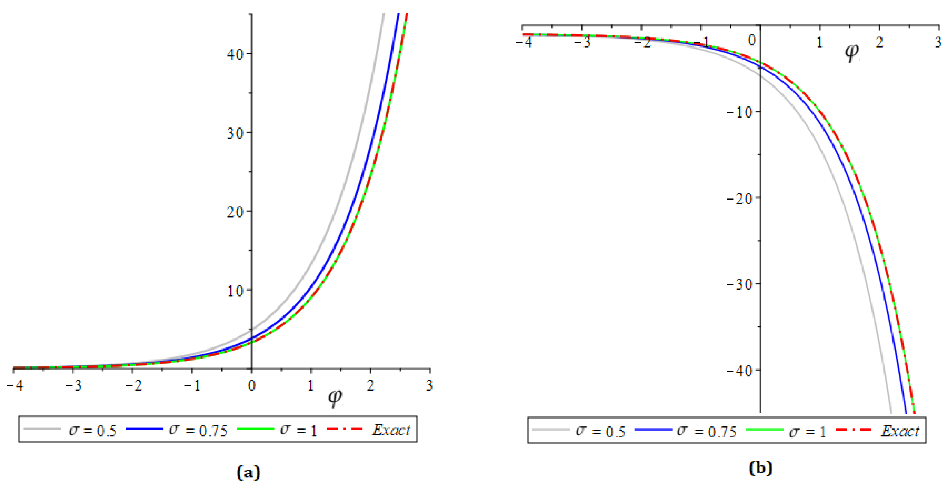
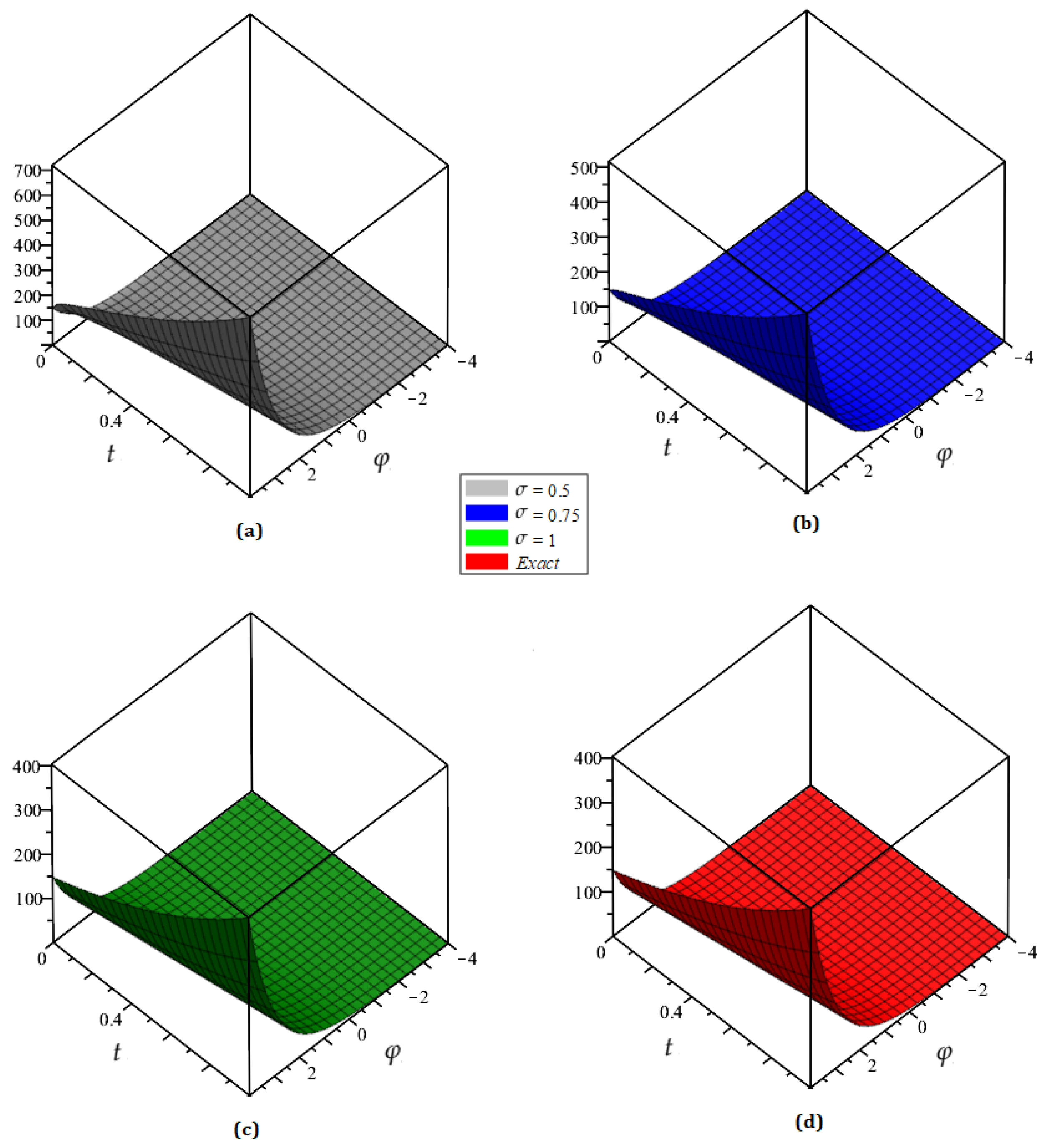
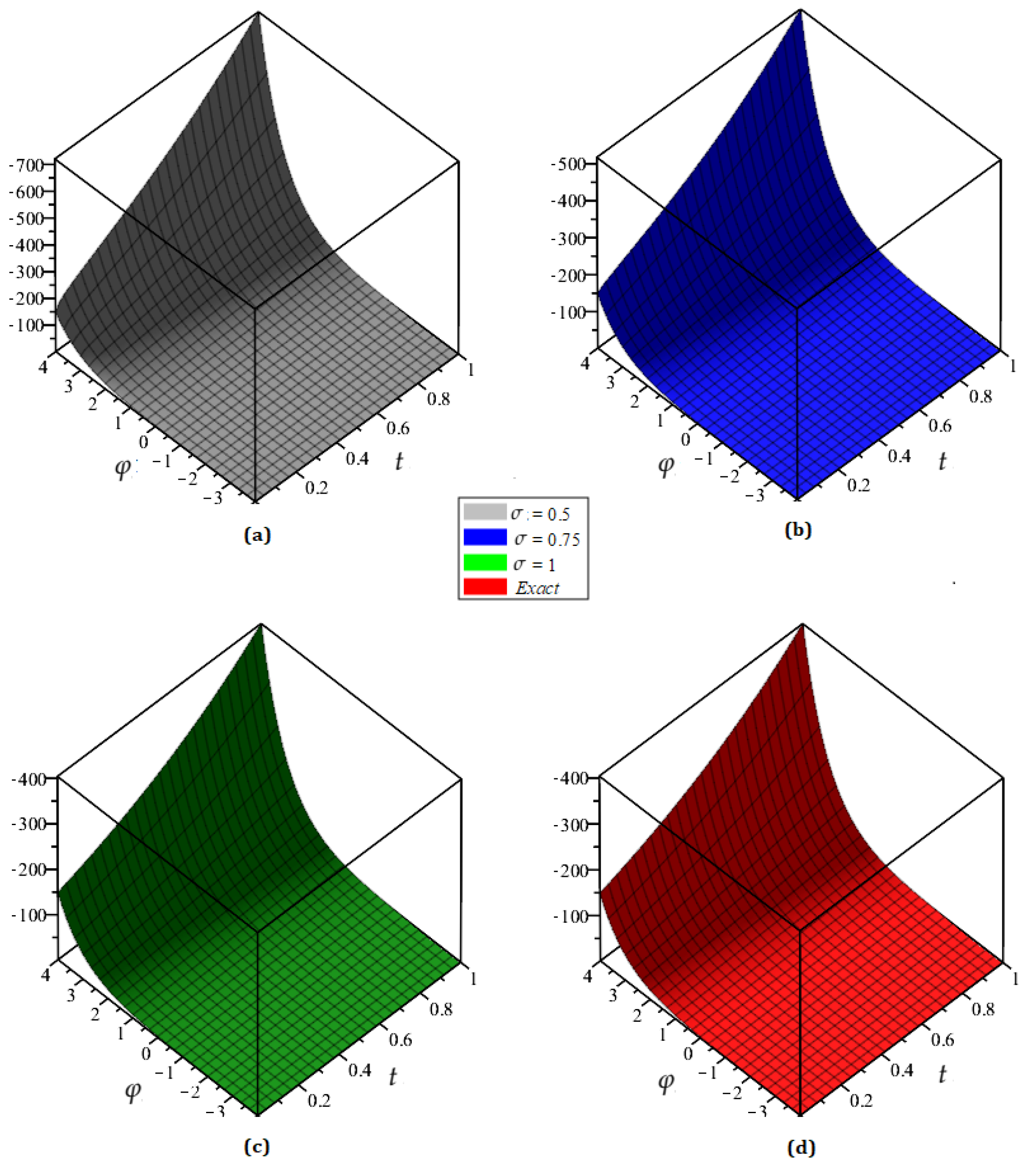
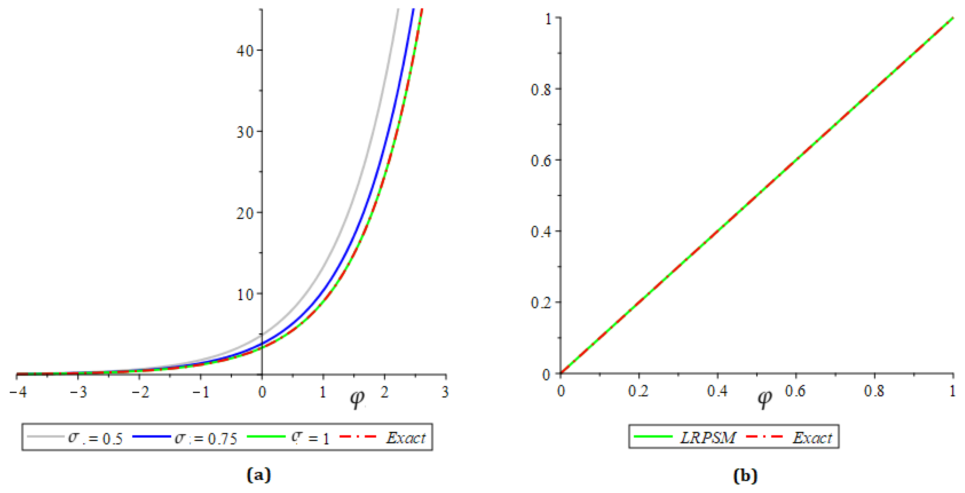
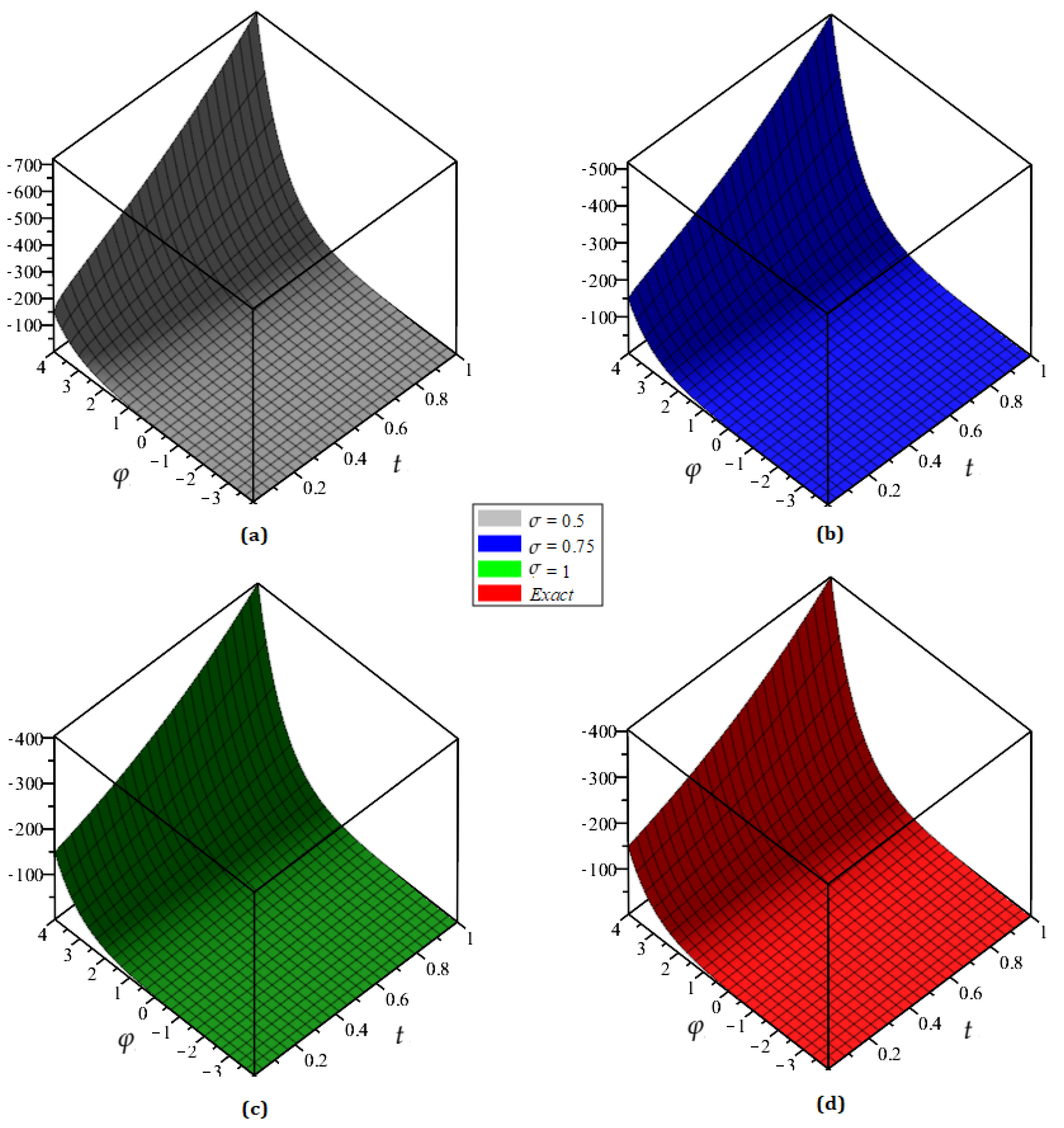
The numerical simulation of the obtained solution for four systems of differential equations describing the unsteady flow of a polytropic gas of arbitrary order is presented in this paper. The sixth-order LRPSM solutions are discovered in this study, which are given in Table 1. The proposed method is more accurate, as shown in the table. For a variety of parameter values, we present 2D and 3D plots to describe the behaviour of the LRPSM solutions. The natures of the LRPSM solutions for and at different orders are represented in Figure 1 as 2D plots, and Figure 2 and Figure 3 represent surfaces of and respectively, and LRPSM solutions for and at different orders are represented in Figure 4 as 2D plots and in Figure 5 as 3D plots for . By simulating and displaying the physical properties of nonlinear phenomena that arise in technology and science, we can study and analyse their physical behaviour. In the analysis of complex coupled fractional-order problems, the suggested technique is more appropriate and efficient.
6. Conclusions
This article presents a combination of the residual power series and Laplace transform to solve the gas dynamics model. The advantage of the new method is that it reduces the amount of computational effort required to obtain a solution in a power series form whose coefficients must be computed in successive algebraic steps. The suggested method is employed to solve three distinct physical models, and its capacity to address fractional nonlinear equations with high precision and simple computation steps has been demonstrated. In future work, we intend to extend the Laplace-transform residual power series technique to physical applications with higher dimensions.
Author Contributions
Data curation, M.M.A.-S. and W.W.; Formal analysis, R.P.A.; Funding acquisition, W.W.; Investigation, M.M.A.-S., O.Y.A. and W.W.; Methodology, R.S.; Software, R.P.A. and R.S.; Supervision, R.P.A.; Visualization, O.Y.A.; Writing—original draft, R.S.; Writing—review & editing, W.W. All authors have read and agreed to the published version of the manuscript.
Funding
This research received no external funding.
Institutional Review Board Statement
Not applicable.
Informed Consent Statement
Not applicable.
Data Availability Statement
Not applicable.
Conflicts of Interest
The authors declare no conflict of interest.
References
- Abdullah, T.Q.S.; Xiao, H.; Huang, G.; Al-Sadi, W. Stability and existence results for a system of fractional differential equations via Atangana-Baleanu derivative with ϕ-p-Laplacian operator. J. Math. Comput. Sci. 2022, 27, 184–195. [Google Scholar] [CrossRef]
- Dousseh, P.Y.; Ainamon, C.; Miwadinou, C.H.; Monwanou, A.V.; Chabi-Orou, J.B. Chaos control and synchronization of a new chaotic financial system with integer and fractional order. J. Nonlinear Sci. Appl. 2021, 14, 372–389. [Google Scholar] [CrossRef]
- Phong, T.T.; Long, L.D. Well-posed results for nonlocal fractional parabolic equation involving Caputo-Fabrizio operator. J. Math. Comput. Sci. 2022, 26, 357–367. [Google Scholar] [CrossRef]
- Oldham, K.; Spanier, J. The Fractional Calculus: Theory and Applications of Differentiation and Integration to Arbitrary Order; Academic Press: New York, NY, USA, 1974. [Google Scholar]
- Miller, K.S.; Ross, B. An Introduction to Fractional Calculus and Fractional Differential Equations; Wiley: New York, NY, USA, 1993. [Google Scholar]
- Podlubny, I. Fractional Differential Equations; Academic Press: New York, NY, USA, 1999. [Google Scholar]
- Kilbas, A.A.; Srivastava, H.M.; Trujillo, J.J. Theory and Applications of Fractional Differential Equations; Elsevier: Amsterdam, The Netherlands, 2006. [Google Scholar]
- Baleanu, D.; Güvenç, Z.B.; Machado, J.A. (Eds.) New Trends in Nanotechnology and Fractional Calculus Applications; Springer: New York, NY, USA, 2010. [Google Scholar]
- Zhang, T.; Li, Y. Exponential Euler scheme of multi-delay Caputo-Fabrizio fractional-order differential equations. Appl. Math. Lett. 2022, 124, 107709. [Google Scholar] [CrossRef]
- Ahmad, S.; Ullah, A.; Akgul, A.; De la Sen, M. A Novel Homotopy Perturbation Method with Applications to Nonlinear Fractional Order KdV and Burger Equation with Exponential-Decay Kernel. J. Funct. Spaces 2021, 2021, 8770488. [Google Scholar] [CrossRef]
- Sun, H.; Zhang, Y.; Baleanu, D.; Chen, W.; Chen, Y. A new collection of real world applications of fractional calculus in science and engineering. Commun Nonlinear Sci. Numer. Simulat. 2018, 64, 213–231. [Google Scholar] [CrossRef]
- Basto, M.; Semiao, V.; Calheiros, F.L. Numerical study of modified Adomian’s method applied to Burgers equation. J. Comput. Appl. Math. 2007, 206, 927–949. [Google Scholar] [CrossRef] [Green Version]
- Adomian, G. Analytical solution of Navier-Stokes flow of a viscous compressible fluid. Found. Phys. Lett. 1995, 8, 389–400. [Google Scholar] [CrossRef]
- Wang, Y.; Zhao, Z.; Li, C.; Chen, Y.Q. Adomian’s method applied to Navier-Stokes equation with a fractional order. In Proceedings of the International Design Engineering Technical Conferences and Computers and Information in Engineering Conferencem, San Diego, CA, USA, 30 August–2 September 2009; pp. 1047–1054. [Google Scholar]
- Roos, H.-G.; Stynes, M.; Tobiska, L. Robust Numerical Methods for Singularly Perturbed Differential Equations; Springer: Berlin/Heidelberg, Germany, 2008; 604p. [Google Scholar]
- Siryk, S.V.; Salnikov, N.N. Construction of Weight Functions of the Petrov-Galerkin Method for Convection-Diffusion-Reaction Equations in the ThreeDimensional Case. Cybern. Syst. Anal. 2014, 50, 805–814. [Google Scholar]
- Stynes, M.; Stynes, D. Convection Diffusion Problems: An Introduction to Their Analysis and Numerical Solution. Am. Math. Soc. 2018, 196, 156p. [Google Scholar]
- Naeem, M.; Azhar, O.F.; Zidan, A.M.; Nonlaopon, K.; Shah, R. Numerical analysis of fractional-order parabolic equations via Elzaki transform. J. Funct. Spaces 2021, 2021, 3484482. [Google Scholar] [CrossRef]
- Salnikov, N.N.; Siryk, S.V.; Tereshchenko, I.A. On construction of finite-dimensional mathematical model of convection-diffusion process with usage of the Petrov-Galerkin method. J. Autom. Inf. Sci. 2010, 42, 67–83. [Google Scholar] [CrossRef]
- John, V.; Knobloch, P.; Novo, J. Finite elements for scalar convection-dominated equations and incompressible flow problems: A never ending story? Comput. Vis. Sci. 2018, 19, 47–63. [Google Scholar] [CrossRef] [Green Version]
- Iqbal, N.; Albalahi, A.M.; Abdo, M.S.; Mohammed, W.W. Analytical Analysis of Fractional-Order Newell-Whitehead-Segel Equation: A Modified Homotopy Perturbation Transform Method. J. Funct. Spaces 2022, 2022, 3298472. [Google Scholar] [CrossRef]
- Daftardar-Gejji, V.; Jafari, H. Solving a Multi-Order Fractional Differential Equation Using Adomian Decomposition. Appl. Math. Comput. 2007, 189, 541–548. [Google Scholar] [CrossRef]
- Elsayed, E.M.; Shah, R.; Nonlaopon, K. The analysis of the fractional-order Navier-Stokes equations by a novel approach. J. Funct. Spaces 2022, 2022, 8979447. [Google Scholar] [CrossRef]
- Bhrawy, A.H. A Jacobi Spectral Collocation Method for Solving Multi-Dimensional Nonlinear Fractional Sub-diffusion Equations. Numer. Algor. 2016, 73, 91–113. [Google Scholar] [CrossRef]
- Biswas, A.; Bhrawy, A.H.; Abdelkawy, M.A.; Alshaery, A.A.; Hilal, E.M. Symbolic. Computation of Some Nonlinear Fractional Differential Equations. Rom. J. Phys. 2014, 59, 433–442. [Google Scholar]
- Iqbal, N.; Botmart, T.; Mohammed, W.W.; Ali, A. Numerical investigation of fractional-order Kersten-Krasil’shchik coupled KdV-mKdV system with Atangana-Baleanu derivative. Adv. Contin. Discret. Model. 2022, 2022, 1–20. [Google Scholar] [CrossRef]
- Mohebbi, A.; Abbaszadeh, M.; Dehghan, M. The Use of a Meshless Technique. Based on Collocation and Radial Basis Functions for Solving the Time. Fractional Nonlinear Schrodinger Equation Arising in Quantum Mechanics. Eng. Anal. Bound. Elem. 2013, 37, 475–485. [Google Scholar] [CrossRef]
- Wang, L.; Ma, Y.; Meng, Z. Haar Wavelet Method for Solving Fractional. Partial Differential Equations Numerically. Appl. Math. Comput. 2014, 227, 66–76. [Google Scholar] [CrossRef]
- Baseri, A.; Babolian, E.; Abbasbandy, S. Normalized Bernstein Polynomials in. Solving Space-Time Fractional Diffusion Equation. Adv. Differ. Equ. 2017, 2017, 1–25. [Google Scholar] [CrossRef] [Green Version]
- Chen, Y.; Sun, Y.; Liu, L. Numerical Solution of Fractional Partial Differential. Equations with Variable Coefficients Using Generalized Fractional-Order. Legendre Functions. Appl. Math. Comput. 2014, 244, 847–858. [Google Scholar] [CrossRef]
- Jafari, H.; Nazari, M.; Baleanu, D.; Khalique, C.M. A New Approach for Solving a System of Fractional Partial Differential Equations. Comput. Math. Appl. 2013, 66, 838–843. [Google Scholar] [CrossRef]
- Maitama, S.; Abdullahi, I. A New Analytical Method for Solving Linear and. Nonlinear Fractional Partial Differential Equations. Progr. Fract. Differ. Appl. 2016, 2, 247–256. [Google Scholar] [CrossRef]
- Jassim, H.K. The Approximate Solutions of Three-Dimensional. Diffusion and Wave Equations within Local Fractional Derivative Operator. In Abstract and Applied Analysis; Hindawi: London, UK, 2016. [Google Scholar]
- Bhrawy, A.H. A New Legendre Collocation Method for Solving a Two-Dimensional Fractional Diffusion Equation. In Abstract and Applied Analysis; Hindawi: London, UK, 2014. [Google Scholar]
- Zhang, Y.; Baleanu, D.; Yang, X. On a Local Fractional Wave Equation under. Fixed Entropy Arising in Fractal Hydrodynamics. Entropy 2014, 16, 6254–6262. [Google Scholar] [CrossRef] [Green Version]
- Shah, N.A.; Alyousef, H.A.; El-Tantawy, S.A.; Chung, J.D. Analytical Investigation of Fractional-Order Korteweg-De-Vries-Type Equations under Atangana-Baleanu-Caputo Operator: Modeling Nonlinear Waves in a Plasma and Fluid. Symmetry 2022, 14, 739. [Google Scholar] [CrossRef]
- Sunthrayuth, P.; Ullah, R.; Khan, A.; Shah, R.; Kafle, J.; Mahariq, I.; Jarad, F. Numerical analysis of the fractional-order nonlinear system of Volterra integro-differential equations. J. Funct. Spaces 2021, 2021, 1537958. [Google Scholar] [CrossRef]
- Mukhtar, S.; Shah, R.; Noor, S. The Numerical Investigation of a Fractional-Order Multi-Dimensional Model of Navier-Stokes Equation via Novel Techniques. Symmetry 2022, 14, 1102. [Google Scholar] [CrossRef]
- Moradpour, H.; Abri, A. Thermodynamic behavior and stability of Polytropic gas. Int. J. Mod. Phys. D 2016, 12. [Google Scholar] [CrossRef] [Green Version]
- Veeresha, P.; Prakasha, D.G.; Baskonus, H.M. An efficient technique for a fractional-order system of equations describing the unsteady flow of a polytropic gas. Pramana 2019, 93, 1–13. [Google Scholar] [CrossRef]
- Iqbal, N.; Akgul, A.; Shah, R.; Bariq, A.; Mossa Al-Sawalha, M.; Ali, A. On solutions of fractional-order gas dynamics equation by effective techniques. J. Funct. Spaces 2022, 2022, 3341754. [Google Scholar] [CrossRef]
- Alaoui, M.K.; Fayyaz, R.; Khan, A.; Abdo, M.S. Analytical investigation of Noyes-Field model for time-fractional Belousov-Zhabotinsky reaction. Complexity 2021, 2021, 3248376. [Google Scholar] [CrossRef]
- Nonlaopon, K.; Naeem, M.; Zidan, A.M.; Alsanad, A.; Gumaei, A. Numerical investigation of the time-fractional Whitham-Broer-Kaup equation involving without singular kernel operators. Complexity 2021, 2021, 7979365. [Google Scholar] [CrossRef]
- Sunthrayuth, P.; Aljahdaly, N.H.; Ali, A.; Mahariq, I.; Tchalla, A.M. Haar Wavelet Operational Matrix Method for Fractional Relaxation-Oscillation Equations Containing-Caputo Fractional Derivative. J. Funct. Spaces 2021, 2021, 7117064. [Google Scholar] [CrossRef]
- Ahmad, E.-A. Adapting the Laplace transform to create solitary solutions for the nonlinear time-fractional dispersive PDEs via a new approach. Eur. Phys. J. Plus 2021, 136, 1–22. [Google Scholar]
- Burqan, A.; El-Ajou, A.; Saadeh, R.; Al-Smadi, M. A new efficient technique using Laplace transforms and smooth expansions to construct a series solution to the time-fractional Navier-Stokes equations. Alex. Eng. J. 2022, 61, 1069–1077. [Google Scholar] [CrossRef]
- El-Ajou, A.; Al-Smadi, M.; Oqielat, M.; Momani, S.; Hadid, S. Smooth expansion to solve high-order linear conformable fractional PDEs via residual power series method: Applications to physical and engineering equations. Ain Shams Eng. J. 2020, in press. [CrossRef]
- El-Ajou, A.; Oqielat, M.; Al-Zhour, Z.; Momani, S. A class of linear non-homogenous higher order matrix fractional differential equations: Analytical solutions and new technique. Fract. Calc. Appl. Anal. 2020, 23, 356–377. [Google Scholar] [CrossRef]
- Aljahdaly, N.H.; Akgul, A.; Mahariq, I.; Kafle, J. A comparative analysis of the fractional-order coupled Korteweg-De Vries equations with the Mittag-Leffler law. J. Math. 2022, 2022, 8876149. [Google Scholar] [CrossRef]
- El-Ajou, A.; Al-Zhour, Z.; Oqielat, M.; Momani, S.; Hayat, T. Series solutions of non- linear conformable fractional KdV-Burgers equation with some applications. Eur. Phys. J. Plus 2019, 134, 402. [Google Scholar] [CrossRef]
- Oqielat, M.; El-Ajou, A.; Al-Zhour, Z.; Alkhasawneh, R.; Alrabaiah, H. Series solu- tions for nonlinear time-fractional Schrödinger equations: Comparisons be- tween conformable and Caputo derivatives. Alexandria Eng. J. 2020, in press. [CrossRef]
- El-Ajou, A.; Oqielat, M.; Al-Zhour, Z.; Momani, S. Analytical numerical solutions of the fractional multi-pantograph system: Two attractive methods and comparisons. Results Phys. 2019, 14, 102500. [Google Scholar] [CrossRef]
- Areshi, M.; Khan, A.; Nonlaopon, K. Analytical investigation of fractional-order Newell-Whitehead-Segel equations via a novel transform. AIMS Math. 2022, 7, 6936–6958. [Google Scholar] [CrossRef]
- Arqub, O.A.; El-Ajou, A.; Momani, S. Construct and predicts solitary pattern solutions for nonlinear time-fractional dispersive partial differential equations. J. Comput. Phys. 2015, 293, 385–399. [Google Scholar] [CrossRef]
- Alquran, M.; Ali, M.; Alsukhour, M.; Jaradat, I. Promoted residual power series technique with Laplace transform to solve some time-fractional problems arising in physics. Results Phys. 2020, 19, 103667. [Google Scholar] [CrossRef]
Figure 1.
Exact and LRPSM solutions for (a) and (b) at distinct values of at and .

Figure 2.
Three-dimensional plots of LRPSM solutions for at distinct values of at . (a) (b) (c) (d) Exact.
Figure 2.
Three-dimensional plots of LRPSM solutions for at distinct values of at . (a) (b) (c) (d) Exact.

Figure 3.
Three-dimensional plots of LRPSM solutions for at distinct values of at . (a) (b) (c) (d) Exact.
Figure 3.
Three-dimensional plots of LRPSM solutions for at distinct values of at . (a) (b) (c) (d) Exact.

Figure 4.
Exact and LRPSM solutions for (a) and (b) at distinct values of at and .

Figure 5.
Three-dimensional plots of LRPSM solutions for at distinct values of at . (a) (b) (c) (d) Exact.
Figure 5.
Three-dimensional plots of LRPSM solutions for at distinct values of at . (a) (b) (c) (d) Exact.


Table 1.
Error analysis for the LRPSM solution for the proposed problem with various values of and t when , .
Table 1.
Error analysis for the LRPSM solution for the proposed problem with various values of and t when , .
| t | |||||
|---|---|---|---|---|---|
| 0.2 | 0.2 | 7.0 | 7.0 | 7.0 | 0 |
| 0.4 | 8.0 | 8.0 | 8.0 | 0 | |
| 0.6 | 1.1 | 1.1 | 1.1 | 0 | |
| 0.8 | 1.4 | 1.4 | 1.4 | 0 | |
| 1 | 1.5 | 1.5 | 1.5 | 0 | |
| 0.4 | 0.2 | 1.134 | 1.134 | 1.134 | 0 |
| 0.4 | 1.385 | 1.385 | 1.385 | 0 | |
| 0.6 | 1.693 | 1.693 | 1.693 | 0 | |
| 0.8 | 2.067 | 2.067 | 2.067 | 0 | |
| 1 | 2.52 | 2.52 | 2.52 | 0 | |
| 0.6 | 0.2 | 1.9921 | 1.9921 | 1.9921 | 0 |
| 0.4 | 2.4333 | 2.4333 | 2.4333 | 0 | |
| 0.6 | 2.9720 | 2.9720 | 2.9720 | 0 | |
| 0.8 | 3.630 | 3.630 | 3.630 | 0 | |
| 1 | 4.434 | 4.434 | 4.434 | 0 |
Publisher’s Note: MDPI stays neutral with regard to jurisdictional claims in published maps and institutional affiliations. |
© 2022 by the authors. Licensee MDPI, Basel, Switzerland. This article is an open access article distributed under the terms and conditions of the Creative Commons Attribution (CC BY) license (https://creativecommons.org/licenses/by/4.0/).
Share and Cite
MDPI and ACS Style
Al-Sawalha, M.M.; Agarwal, R.P.; Shah, R.; Ababneh, O.Y.; Weera, W. A Reliable Way to Deal with Fractional-Order Equations That Describe the Unsteady Flow of a Polytropic Gas. Mathematics 2022, 10, 2293. https://doi.org/10.3390/math10132293
AMA Style
Al-Sawalha MM, Agarwal RP, Shah R, Ababneh OY, Weera W. A Reliable Way to Deal with Fractional-Order Equations That Describe the Unsteady Flow of a Polytropic Gas. Mathematics. 2022; 10(13):2293. https://doi.org/10.3390/math10132293
Chicago/Turabian StyleAl-Sawalha, M. Mossa, Ravi P. Agarwal, Rasool Shah, Osama Y. Ababneh, and Wajaree Weera. 2022. "A Reliable Way to Deal with Fractional-Order Equations That Describe the Unsteady Flow of a Polytropic Gas" Mathematics 10, no. 13: 2293. https://doi.org/10.3390/math10132293
Note that from the first issue of 2016, this journal uses article numbers instead of page numbers. See further details here.