Article

A Novel Fractional-Order Discrete SIR Model for Predicting COVID-19 Behavior

1
Department of Mathematics and Computer Science, University of Larbi Ben M’hidi, Oum El Bouaghi 04000, Algeria
2
Nonlinear Dynamics Research Center (NDRC), Ajman University, Ajman 346, United Arab Emirates
3
Department of Mathematics, Faculty of Science and Technology, Irbid National University, Irbid 2600, Jordan
4
Dipartimento Ingegneria Innovazione, Universita del Salento, 73100 Lecce, Italy
5
Department of Mathematics, Faculty of Science, University of Jordan, Amman 11942, Jordan
*
Author to whom correspondence should be addressed.
Mathematics 2022, 10(13), 2224; https://doi.org/10.3390/math10132224
Submission received: 17 April 2022 / Revised: 14 June 2022 / Accepted: 22 June 2022 / Published: 25 June 2022
(This article belongs to the Special Issue Q-differential/Difference Equations and Related Applications)

Abstract

:
During the broadcast of Coronavirus across the globe, many mathematicians made several mathematical models. This was, of course, in order to understand the forecast and behavior of this epidemic’s spread precisely. Nevertheless, due to the lack of much information about it, the application of many models has become difficult in reality and sometimes impossible, unlike the simple SIR model. In this work, a simple, novel fractional-order discrete model is proposed in order to study the behavior of the COVID-19 epidemic. Such a model has shown its ability to adapt to the periodic change in the number of infections. The existence and uniqueness of the solution for the proposed model are examined with the help of the Picard Lindelöf method. Some theoretical results are established in view of the connection between the stability of the fixed points of this model and the basic reproduction number. Several numerical simulations are performed to verify the gained results.

1. Introduction

Across the centuries, the world has seen the dissemination of several diseases, which have caused extensive loss of lives. In the first quarter of 2020, the World Health Organization (WHO) declared the COVID-19 pandemic around the world [1]. From such time up to now, the total number of global deaths has surpassed the obstacle of 5 million deaths. The world was compelled to track many preventive strategies such as using masks, sanitizers and imposing quarantine.
In terms of a mathematician’s view, it is still essential to establish a proper mathematical model that can describe the growth of the COVID-19 pandemic and its effects on communities, see [2,3,4,5,6,7,8,9]. As a matter of fact, the Susceptible-Infectious-Removed model (or simply SIR model) is deemed one of the most distinguished mathematical models, which can be typically employed to outline the dynamics of such pandemic and evaluate possible scenarios of infection. The SIR model can be extremely useful for assessing the effectiveness of numerous strategies. This model depends in its construction on a kind of ordinary differential equations that consider the total population with respect to its infection, the persons who unfortunately die, and the direction of persons who recover after infection over a given time [10,11].
In mathematical modeling, the ordinary differential equations are commonly utilized to establish certain models of continuous-time mode, whereas the difference equations are, on the other hand, utilized to establish other models of discrete-time mode. Regarding the continuous-time models, we find that there are some pioneer works that have recently dealt with the COVID-19 disease in very practical manners. For instance, a novel version of time-dependent SIR model was recently constructed in [12] to investigate the transmission rate of COVID-19 disease in various regions of India, where such model was employed to show the effect of the complete knockdown on the transmission rate of the COVID-19 infection in Indian districts with the help of ArcGIS 10.2 by preparing district-wise spatial distribution maps. In [13], another fractional-order SIR model was derived from the stochastic process of a continuous-time random walk that incorporates a time-since-infection dependence on both the infectivity and the recovery of the population. In [14], several infectious diseases, including COVID-19 in its SIR form, were analyzed with the application of mathematical modeling in the analysis of their spreading rates and treatments. In [15], certain random walk models for the daily time series that confirmed COVID-19 cases for different countries were introduced and discussed, where such model was derived from the evolutionary equation for a specified memory function that can provide some non-ergodic fields, which were evident in some available COVID-19 data. At the same time, the discrete-time models have been recently employed to assess and explore the infectious diseases instead of the continuous-time models, as pandemic data are accessible during the periods of discrete-time [16]. In addition, the discrete-time models can demonstrate more rich dynamics than the continuous-time ones. In order to provide an overview of some kinds of discrete models, the reader may refer to [17,18,19,20]. In particular, a discrete SIR epidemic model with a constant vaccination strategy in terms of its dynamical behavior was examined in [21], whereas the authors in [22] investigated the bifurcations and stability of a proposed discrete-time model of a susceptible-infected-susceptible (SIS) mode with vaccination. In addition, another proposed discrete-time model with vaccination was examined in terms of its dynamical behavior by Xiang et al. in [23]. In the same regard, a new generalization version of the fractional-order SIR epidemic model for predicting the spread of the COVID-19 disease was presented in [24], where the time-domain model implementation was based on the fixed-step method using the nabla fractional-order difference Grünwald-Letnikov operator.
In mathematical analysis, fractional calculus is considered one of the most important subjects as a generalization of integer calculus [25,26,27,28,29,30]. It has been demonstrated that the fractional-order derivative is significantly more precise than the integer-order one [31]. This is because it plays a key role as a powerful tool for outlining the effect of memory on all kinds of materials and processing [32]. From the perspective of this view, a lot of researchers have, over the last several years, been concerned with discrete fractional calculus [33,34,35,36,37]. In fact, there are many applications of such field in reality, such as the applications connected with biology, physics, neural networks, etc.
In the past few years, many epidemiology SIR models have been established in view of fractional-order differential equations [38,39,40]. In particular, a fractional-order SIR model was investigated in terms of its stability in implementing a discretization scheme in [41]. Naik proposed another fractional-order SIR model in terms of its global dynamics in [42]. Several numerical simulations with their analysis were performed for a new fractional-order SIR model in [43]. A delayed incommensurate fractional-order SIR model was also examined in terms of its bifurcation control and stability analysis in [44]. In view of the above considerations, it should be emphasized that all the aforesaid studies were established based on a continuous-time mode. This actually motivated us to propose a new fractional-order discrete model to be considered in the epidemiology field. As far as we know, the study of fractional-order discrete-time COVID-19 models has not probably been explored till now. Thus, from this perspective, the main target of this work is to make a contribution to the epidemiology field by proposing a new fractional-order discrete-time SIR model. In this regard, it is worth mentioning that due to the fact the proposed model is just a fractionalization of the discrete SIR-type system and due to the pandemic time series that can be generated from its dynamics, we believe that this model will, in general, have several potential applications and perspectives.
In fact, in order to formulate the target mathematical model, which will enable us later to predict the COVID-19 behavior according to the available information, we suppose that the society is divided into four different classes; susceptible class S, infected class I, recovered class R and death class D. In addition, we suppose that the transition between these classes takes place according to the scheme exhibited in Figure 1.
In light of this figure, the values of all parameters reported in the model at hand can be explained, as shown in Table 1.
As a matter of fact, the disease transmission flow of the proposed fractional-order discrete SIR model, which is shown in its compartmental form in Figure 1, can be furthermore described by the following nonlinear system:
S ( n + 1 ) = S ( n ) + θ + η R ( n ) b S ( n ) I ( n ) δ S ( n ) , I ( n + 1 ) = I ( n ) + b S ( t ) I ( n ) μ + δ + e I ( n ) , R ( n + 1 ) = R ( n ) + e I ( n ) δ + η R ( n ) , D ( n + 1 ) = D ( n ) + μ I ( n ) ,
subject to the following initial conditions:
S ( 0 ) , I ( 0 ) , R ( 0 ) , D ( 0 ) 0 .
Since the first three equations in the proposed system (1) are not related to class D, and because this class can be studied alone from using the equation:
N ( n ) = S ( n ) + I ( n ) + R ( n ) + D ( n ) ,
then the last equation of system (1) might be ignored. This would actually facilitate our examination by focusing only on the first three equations of that system. At the same time, it should be noted that because the value of the parameter b is very small ( b = p k N , where k is the rate of contacts per unit of time so 0 k 1 , p is the probabilities of contagion so 0 p 1 , and N is the number of the total population in the tens of thousands or more), the two terms b S ( n ) and b I ( n ) are also very small. The fact that we did not mention the age groups and vaccination does not mean that they were neglected, but the high life expectancy in a society can be seen as one of the causes of the high death rate due to the virus. As for vaccination, we know that it does not provide 100 percent immunity, but it reduces the possibility of infection (which reduces b), reduces virus mortality ( η ), and increases the recovery rate (e).
The rest of this paper is organized as follows: Section 2 recalls some basic definitions and primary facts associated with discrete fractional calculus. In Section 3, we use the fixed point theory coupled with the Picard Lindelöf method for the purpose of showing the existence and uniqueness of the solution for the proposed fractional-order discrete-time COVID-19 model. In Section 4, we analyze the stability of the fixed points of the proposed model, and we find the basic reproduction number of an infectious disease. Section 5 shows several numerical simulations performed to verify the theoretical findings, followed by Section 6, which summarizes the conclusions of this work.

2. Preliminaries

During the past few decades, fractional calculus has demonstrated high efficiency in providing more practical outcomes than that of traditional calculus. This, actually, is due to its flexibility and ability to provide approximations of several phenomena better than before. However, in order to gain more depth in understanding the proposed fractional-order model in this work and its impact on reality, it is useful to outline some definitions and basic facts connected with discrete fractional calculus. From now on, we will assume that all functions are defined on the set N a : = { a , a + 1 , a + 2 , } , where a R .
Definition 1
([45]). The α t h -fractional sum of the function f : N a R is defined by:
Δ a α f ( t ) = 1 Γ ( α ) s = a t α ( t s 1 ) ( α 1 ) f ( s ) , for t N a + α ,
where α > 0 , Γ ( · ) is the Euler’s gamma function and t ( α ) = Γ ( t + 1 ) Γ ( t + 1 α ) .
Definition 2
([45]). The α t h -order Rimann–Liouville fractional difference operator of the function f defined on N a is outlined by:
Δ a α f ( t ) : = Δ Δ a ( 1 α ) f ( t ) = 1 Γ ( 1 α ) Δ s = a t ( 1 α ) ( t s 1 ) ( α ) f ( s ) , for t N a + 1 α ,
where 0 < α < 1 .
Definition 3
([45]). The α t h -order Caputo fractional difference operator of the function f defined on N a is outlined by:
C Δ a α f ( t ) = Δ a ( 1 α ) Δ f ( t ) = 1 Γ ( 1 α ) s = a t ( 1 α ) ( t s 1 ) ( α ) Δ f ( s ) , 0 < α < 1 Δ f ( t ) , α = 1 ,
where 0 < α 1 and t N a + 1 α .
Proposition 1
([45]). Let f be a function defined on N a . Then:
Δ a + ( 1 α ) α C Δ a α f ( t ) = f ( t ) f ( a ) , t N a ,
where 0 < α 1 .
Proposition 2
([45]). Let f be a function defined on N a . Then:
C Δ a α f ( t ) = Δ a α f ( t ) ( t a ) ( α ) Γ ( 1 α ) f ( a ) , t N a α + 1 ,
where 0 < α < 1 .
Lemma 1
([46]). Let α > 0 , α N and f be a function defined on N a . Then:
f ( t ) = f ( a ) + 1 Γ ( α ) t α r = a + 1 α ( t r 1 ) ( α 1 ) C Δ a α f ( r ) , t N a + 1 .
Remark 1.
One might observe the following states:
  • If C Δ a α f ( t ) 0 , then the function f is nondecreasing for all t N a .
  • If C Δ a α f ( t ) 0 , then the function f is nonincreasing for all t N a .
Theorem 1
([47]). Suppose h ( t , y ) and k ( t , y ) are two real-valued functions defined on [ 0 , + ) × R . If the function k satisfies the Lipschitz condition in y with Lipschitz constant L k such that 0 < L k α , then y 1 ( t ) and y 2 ( t ) are, respectively, two unique solutions for the following initial value problems:
Δ a α y ( t ) = h ( t + α 1 , y ( t + α 1 ) ) , t N a + 1 α Δ a α 1 y ( t ) t = a = y 0 ,
and
Δ a α y ( t ) = k ( t + α 1 , y ( t + α 1 ) ) , t N a + 1 α Δ a α 1 y ( t ) t = a = y 0 .
Herein, based on the above theorem, it can be noted the following observations:
  • If h ( t , y ) < k ( t , y ) , then y 1 ( t ) y 2 ( t ) for t N a .
  • If h ( t , y ) > k ( t , y ) , then y 1 ( t ) > y 2 ( t ) for t N a .
Remark 2.
In view of Proposition 2, we can notice that Theorem 1 remains true if we replace Δ a α by C Δ a α .
In accordance with the nonlinear model given in (3), we can now define the fractional-order model, which will be taken into consideration in this work from now on. This model has the following form:
C Δ 0 α S ( t + 1 α ) = θ + η R ( t ) b S ( t ) I ( t ) δ S ( t ) , C Δ 0 α I ( t + 1 α ) = b S ( t ) I ( t ) μ + δ + e I ( t ) , C Δ 0 α R ( t + 1 α ) = e I ( t ) δ + η R ( t ) ,
subject to the following initial conditions:
S ( 0 ) , I ( 0 ) , R ( 0 ) , D ( 0 ) 0 ,
where 0 < α < 1 and t N . Continuing to move forward in our examination, we recall below an important result that clarifies the stability of the solution of system (12).
Theorem 2
([48,49]). Let α ( 0 , 1 ) . If
λ z C : z < 2 cos arg z π 2 α α and arg z > α π 2 ,
for all the eigenvalues λ of J, then the fixed point of system (12) is asymptotically stable, where J is the Jacobite matrix of the second member of system (12) at the fixed point itself.

3. Existence and Uniqueness

In the following content, we intend to use the fixed point theory together with the Picard Lindelöf method to show the existence and uniqueness of solution for system (12). For this purpose, we may rewrite such system in the following classical form:
C Δ 0 α X ( t ) = F ( t 1 + α , X ( t 1 + α ) ) , X ( 0 ) = X 0 ,
where t N 1 α T max in which T max 1 + α N , X ( t ) = ( S ( t ) , I ( t ) , R ( t ) , D ( t ) ) T and the function F ( t , X ( t ) ) is defined as follows:
F 1 ( t , S ) = θ + η R ( t ) b S ( t ) I ( t ) δ S ( t ) , F 2 ( t , I ) = b S ( t ) I ( t ) μ + δ + e I ( t ) , F 3 ( t , R ) = e I ( t ) δ + η R ( t ) .
In order to proceed with the existence and uniqueness investigation, we use the initial condition X ( 0 ) as well as Proposition 1. This would immediately transform system (12) into the following sum equations:
S ( t ) S ( 0 ) = Δ 1 α α θ + η R ( t ) b S ( t ) I ( t ) δ S ( t ) , I ( t ) I ( 0 ) = Δ 1 α α b S ( t ) I ( t ) μ + δ + e I ( t ) , R ( t ) R ( 0 ) = Δ 1 α α e I ( t ) δ + η R ( t ) ,
for t N 1 α T max . Using system (17) and Definition 1, we can obtain the state variable in terms of F i ( t , X ( t ) ) , where i = 1 , 2 , 3 . In other words, we have:
S ( t ) = S ( 0 ) + 1 Γ ( α ) s = 1 α t α ( t s 1 ) ( α 1 ) F 1 ( s 1 + α , S ( s 1 + α ) ) , I ( t ) = I ( 0 ) + 1 Γ ( α ) s = 1 α t α ( t s 1 ) ( α 1 ) F 2 ( s 1 + α , I ( s 1 + α ) ) , R ( t ) = R ( 0 ) + 1 Γ ( α ) s = 1 α t α ( t s 1 ) ( α 1 ) F 3 ( s 1 + α , R ( s 1 + α ) ) , t N 1 T max .
Thus, with the help of Picard iterations, we can obtain the following equations:
S n + 1 ( t ) = S ( 0 ) + 1 Γ ( α ) s = 1 α t α ( t s 1 ) ( α 1 ) F 1 ( s 1 + α , S n ( s 1 + α ) ) , I n + 1 ( t ) = I ( 0 ) + 1 Γ ( α ) s = 1 α t α ( t s 1 ) ( α 1 ) F 2 ( s 1 + α , I n ( s 1 + α ) ) , R n + 1 ( t ) = R ( 0 ) + 1 Γ ( α ) s = 1 α t α ( t s 1 ) ( α 1 ) F 3 ( s 1 + α , R n ( s 1 + α ) ) , t N 1 T max .
Consequently, based on system (17), together with its initial condition, we can gain the following sum equation:
X ( t ) = X ( 0 ) + 1 Γ ( α ) s = 1 α t α ( t s 1 ) ( α 1 ) F ( s 1 + α , X ( s 1 + α ) ) ,
where t N 1 . As a result of the previous groundwork, we can infer the following theoretical results that concern the existence and uniqueness of a solution for the system at hand.
Lemma 2.
The function F ( t , X ( t ) ) defined in (16) satisfies the following Lipschitz condition:
F ( t , X ( t ) F ( t , X * ( t ) ) β X ( t ) X * ( t ) ,
where
β = max max b S ( t ) μ + δ + e , max δ + b I ( t ) , δ + η .
Proof. 
By taking S ( t ) and S * ( t ) as two coupled functions, we obtain:
F 1 ( t , S ) F 1 ( t , S * ) = δ + b I ( t ) S S * .
At the same time, by taking into account:
β 1 = max δ + b I ( t ) ,
one can reach:
F 1 ( t , S ) F 1 ( t , S * ) β 1 S S * .
Continuing in a similar manner yields the following two inequalities:
F 2 ( t , I ) F 2 ( t , I * ) β 2 I I * , F 3 ( t , R ) F 3 ( t , R * ) β 3 R R * ,
where
β 2 = max b S ( t ) μ + δ + e , β 3 = δ + η .
From (24)–(26), we can confirm that the kernels F 1 , F 2 and F 3 satisfy the Lipschitz condition. Moreover, if β i < 1 , then the kernel F i is a contraction for i = 1 , 2 , 3 . □
Theorem 3.
Assume that condition (21) is satisfied, then there exists a unique solution of system (12) if:
( T max 1 + α ) ( α ) Γ ( α + 1 ) β < 1 .
Proof. 
Actually, the solution of system (12) can be outlined as:
X ( t ) = P ( X ( t ) ) ,
where P is the Picard operator defined by:
P ( X ( t ) ) = X ( 0 ) + 1 Γ ( α ) t α s = 1 α ( t s 1 ) ( α 1 ) F ( s 1 + α , X ( s 1 + α ) ) .
Based on the previous arguments, we can have:
P ( X 1 ( t ) P ( X 2 ( t ) ) = 1 Γ ( α ) s = 1 α t α ( t s 1 ) ( α 1 ) ( F ( s 1 + α , X 1 ( s 1 + α ) ) F ( s 1 + α , X 2 ( s 1 + α ) ) ) , 1 Γ ( α ) s = 1 α t α ( t s 1 ) ( α 1 ) ( F ( s 1 + α , X 1 ( s 1 + α ) ) F ( s 1 + α , X 2 ( s 1 + α ) ) ) , 1 Γ ( α ) s = 1 α t α ( t s 1 ) ( α 1 ) max s N 1 α t α ( F ( s 1 + α , X 1 ( s 1 + α ) ) F ( s 1 + α , X 2 ( s 1 + α ) ) ) , ( t 1 + α ) ( α ) Γ ( α + 1 ) β X 1 ( t ) X 2 ( t ) .
Since ( T max 1 + α ) ( α ) Γ ( α + 1 ) β < 1 , then the operator P is a contraction, where t T max . Hence, system (12) has a unique solution. □
In this regard and based on the aforesaid discussion, we can deduce, for the population size N = S + I + R , the following assertion:
C Δ a α N ( t + 1 α ) = θ δ N ( t ) μ + γ I ( t ) θ δ N ( t ) .
This, consequently, yields:
C Δ a α N ( t + 1 α ) C Δ a α Y ( t + 1 α ) ,
where
C Δ a α Y ( t + 1 α ) = θ δ Y ( t ) , Y ( a ) = N ( a ) .
Thus, with the help of using Theorem 1 and Remark 2, it follows that:
N ( t ) Y ( t ) ,
that is because N ( a ) θ δ . Now, if we assume t * N a is the first point, where Y ( t * ) > θ δ , then we have:
Y ( t * ) = Y ( a ) + 1 Γ ( α ) r = a + 1 α t * α ( t * r 1 ) ( α 1 ) C Δ a α Y ( r ) = Y ( a ) + 1 Γ ( α ) r = a + 1 α t * 1 α ( t * r 1 ) ( α 1 ) C Δ a α Y ( r ) + ( α 1 ) ( α 1 ) Γ ( α ) C Δ a α Y ( t * α ) = Y ( a ) + 1 Γ ( α ) r = a + 1 α t * 1 α ( t * r 1 ) ( α 1 ) C Δ a α Y ( r ) + ( α 1 ) ( α 1 ) Γ ( α ) C Δ a α Y ( t * α ) = Y ( a ) + 1 Γ ( α ) r = a + 1 α t * 1 α ( t * r 1 ) ( t * r α ) ( t * r 2 ) ( α 1 ) C Δ a α Y ( r ) + ( α 1 ) ( α 1 ) Γ ( α ) C Δ a α Y ( t * α ) = Y ( t * 1 ) + 1 Γ ( α ) r = a + 1 α t * 1 α ( α 1 ) ( t * r α ) ( t * r 2 ) ( α 1 ) C Δ a α Y ( r ) + ( α 1 ) ( α 1 ) Γ ( α ) C Δ a α Y ( t * α ) Y ( t * 1 ) + θ δ Y ( t * 1 ) θ δ , if δ < 1 .
Thus, we have a contradiction. Therefore, from this result, we can also prove that if δ < 1 , then we can have:
Y ( t ) 0 .
This, actually, asserts that the solution of the system belongs to the region:
X R 3 , 0 x 1 + x 2 + x 3 θ δ .
It is worth mentioning that the solution of System (3) is positive when b is small enough. However, it can not be shown that the solution of system (12) is positive. Actually, the solution of this system sometimes has negative values, but it can then increase to have positive values once again. For example, if we let t * be the first point at which S becomes negative, we obtain:
C Δ 0 α S ( t * + 1 α ) = θ δ S ( t * ) b S ( t * ) I ( t * ) + η R ( t * ) > 0 .
Thus, in accordance with Remark 1, one can notice that the class S will then be increased immediately. This assertion can be, in a similar manner, proven for the two classes I and R. Although this matter is considered a paradox because the values of the system should not be negative, what has been observed is that this system can give more realistic results over time. However, this inference will be discussed later on.

4. Fixed Points and Stability Analysis

In this section, we will be concerned with analyzing the stability of the disease-free fixed point by finding sufficient conditions connected with the parameters of system (12) to ensure the stability of this point. To this aim, we will first find those fixed points by equating the right-hand side of system (12) with zero. In other words, we have:
θ + η R * b S * I * δ S * = 0 , b S * I * μ + δ + e I * = 0 , e I * δ + η R * = 0 .
It can be then seen that the above system has two fixed points at most. The first one is called the disease-free fixed point (or simply DFF point), which can be obtained by assuming I * = 0 , i.e.,
E 0 = θ δ , 0 , 0 .
On the other hand, if we let I * 0 , then we obtain:
R * = e δ + η I * S * = μ + δ + e b , I * = δ μ + δ + e b θ b δ + η η e δ + η μ + δ + e .
This, actually, yields the second fixed point of the considered system, which is called the pandemic fixed point E * . In other words, this point can be yielded only when I * > 0 , and it has the form E * = ( S * , I * , R * ) , where S * , I * and R * are defined above.
In the same regard, the so-called basic reproduction number R 0 can be defined as the number of infections caused by the first disease case. This ’infections’ number typically appears in an appointed population where everyone is assumed to be susceptible to infection [40]. The importance of R 0 lies in knowing the rapidity of the spread of the emerging disease among the inhabitants and the proportion of the population to be immunized [40]. To be precise, the population spread of the epidemic will occur when R 0 > 1 , where it is difficult to control. The method to enumerate the basic reproduction number can be performed by finding the spectral radius of the next generation matrix Y (i.e., R 0 = ρ ( Y ) ). The matrix Y is a multiplication of F by V 1 , where:
F = F i ( E 0 ) t j and V = V i ( E 0 ) t j ,
where F i refers to the stream of freshly infected cases into compartment t j , and V i refers to the entering/leaving streams connected with t j , for i , j = 1 , 2 , 3 , , m such that m is the total of compartments demonstrated in the model. Based on the aforesaid argument, one might calculate R 0 for the fractional-order model (12) by obtaining the two primary matrices F and V. To this aim, we can note that the infected compartment I can yield the following assertion:
C Δ a α I ( t + 1 α ) = b S ( t ) I ( t ) μ + δ + e I ( t ) .
This consequently implies the following Jacobian matrix:
J = b θ δ μ + δ + e .
Accordingly, the above matrix can be decomposed in terms of the two matrices F and V so that J = F V , where:
F = b θ δ ,
and
V = μ + δ + e .
Therefore, the basic reproduction number R 0 can be then calculated to be given as:
R 0 = ρ ( Y ) = ρ ( F V 1 ) = b θ δ μ + δ + e .
Remark 3.
It should be noted that:
I * = δ + η θ μ + δ + e δ + η η e 1 1 R 0 ,
which asserts that the pandemic fixed point E * will hold only when R 0 > 1 .
In what follows, we will analyze the stability of the DFF point. This will be implemented by establishing some sufficient conditions related to the parameters of system (12) to ensure the stability of this point. In order to achieve this objective, we introduce the next theoretical result.
Theorem 4.
In case of R 0 < 1 , the DFE point ( E 0 ) of system (12) is locally asymptotically stable if
max δ + μ + e 1 R 0 , δ + η < 2 α .
Proof. 
The Jacobian matrix of F at E 0 can be given as:
J ( E 0 ) = δ b θ δ η 0 b θ δ μ + δ + e 0 0 e δ + η .
Consequently, the characteristic polynomial will be as:
det λ I d J ( E 0 ) = λ + δ λ + δ + η λ + δ e b θ + δ 2 + μ δ δ ,
det λ I d J ( E 0 ) = λ + δ λ + δ + η λ δ + μ + e R 0 1 .
This implies:
det λ I d J ( E 0 ) = 0 ,
λ 1 = δ < 0
λ 2 = δ + η < 0
and
λ 3 = δ + μ + e R 0 1 < 0 .
Thus, when R 0 < 1 , we have:
2 α < λ 1 < 0 2 α < λ 2 < 0 .
Hence, according to Theorem 2, the DFE point is locally asymptotically stable if R 0 < 1 . □

5. Application to Predict the Behavior of COVID-19 in Germany

In this section, we will perform several numerical simulations to verify the results inferred in the previous sections. For this purpose, we will apply our study to predict the behavior of the virus in Germany. We will take all the statistics of a million people, which means we will take the initial population size N ( 0 ) as 1,000,000. According to [50], we can easily find: the number of new births per day for a million people θ = 26.3308 and the death rate δ = 3.15 × 10 5 . We can also obtain the stats described in Table 2 from the site [51].
Using Table 2 and [51], we find the contact rate b = 5.1160 × 10 7 , the recovery rate e = 0.0789 , the rate at which a recovering person is at risk of infection η = 0.87 , and the corona death rate μ = 0.1 . We also find that the initial number of the susceptible people is S ( 0 ) = 686,400, while the initial number of the exposed people is I ( 0 ) = 33,966, and finally, the initial number of the infected people is R ( 0 ) = 279,630. In order to apply Theorem 4, we first calculate the basic reproduction number:
R 0 = b θ δ μ + δ + e = 0.73013 < 1 ,
and
max δ + μ + e 1 R 0 , δ + η < 2 α = 0.87003 < 2 α .
Note that the conditions of Theorem 4 are validated, then the DFE point is locally asymptotically stable. Anyhow, based on these, we plot Figure 2 and Figure 3, which represents a numerical simulation, confirming the stability of the system (12) in this case.
In order to obtain a better modeling use the incommensurate order system
C Δ 0 α 1 S ( t + 1 α ) = θ + η R ( t ) b S ( t ) I ( t ) δ S ( t ) , C Δ 0 α 2 I ( t + 1 α ) = b S ( t ) I ( t ) μ + δ + e I ( t ) , C Δ 0 α 3 R ( t + 1 α ) = e I ( t ) δ + η R ( t ) ,
where 0 α 1 , α 2 , α 3 1 . In this case, the existence of a direct and simple condition that deals with the stability of the system (56) is difficult and may be impossible in comparison with establishing a simple condition that deals with the stability of the commensurate system (12). However, it can indeed study the stability of the fixed points for system (56) by knowing the values of α i , 1 i 3 . In such a case, we need to report the next corollary.
Corollary 1
([48]). Suppose that 0 < α i < 1 , for 1 i 3 , and M is the least common multiple of u i and v i so that α i = v i u i with g c d ( u i , v i ) = 1 and 1 i 3 , where g c d ( · , · ) is denoted to the greatest common divisor. If at least one root of the following equation:
det d i a g ( λ M α 1 , λ M α 2 , λ M α 3 ) 1 λ M J = 0 ,
lies inside the set
C K 1 M ,
then the trivial solution of system (56) corresponding to S ( 0 ) , E ( 0 ) , I ( 0 ) is locally asymptotically stable, where
K 1 M = z C : z 2 cos M arg z 1 M and arg z π 2 M .
Overall we will consider α 1 = 0.223 , α 2 = 0.2 , α 3 = 0.232 . In this case, we obtain a more accurate approximation than the commensurate order case. Figure 4 shows a numerical simulation of this case, and Figure 5 represents the comparison of this case with the real data, while Figure 6 represents the comparison between the integer order case, the commensurate order case, the incommensurate order case, and the real data. It can be seen that each time, the system is more accurate.
It can be seen that system (56) is more accurate than system (12), and this reduces the error rate in prediction.

6. Conclusions

In this work, a novel fractional-order discrete model has been proposed with the aim of studying the behavior of the COVID-19 pandemic. With the help of using the Picard Lindelöf method, the existence and uniqueness of the solution for the proposed model have been investigated. In light of the relationship between the stability of the fixed points of this model and the basic reproduction number, some useful theoretical results have been established. To verify these results, several numerical simulations have been performed via MATLAB scripts. In general, we can assert that the presented model in this work can be applied to study the COVID-19 pandemic in many regions around the world, even if this model is formulated with the fractional-order backward operator in its commensurate or incommensurate cases.

Author Contributions

Conceptualization, S.M.; Data curation, A.O.; Formal analysis, N.D.; Funding acquisition, G.G.; Methodology, A.O., I.M.B. and T.-E.O.; Resources, T.-E.O.; Software, I.M.B.; Supervision, G.G.; Validation, S.M.; Visualization, N.D. All authors have read and agreed to the published version of the manuscript.

Funding

This research received no external funding.

Institutional Review Board Statement

Not applicable.

Informed Consent Statement

Not applicable.

Data Availability Statement

The data that support the findings of this study are openly available in [World Matter] at [https://www.worldometers.info/, accessed on 15 June 2022] and [World Health Organization] at [https://www.who.int/emergencies/diseases/novel-coronavirus-2019, accessed on 15 June 2022].

Conflicts of Interest

The authors declare no conflict of interest.

References

  1. World Health Organization (WHO). Coronavirus Disease (COVID-19) Outbreak Situation. Available online: https://www.who.int/emergencies/diseases/novel-coronavirus-2019 (accessed on 17 December 2020).
  2. Albadarneh, R.B.; Batiha, I.M.; Ouannas, A.; Momani, S. Modeling COVID-19 Pandemic Outbreak using Fractional-Order Systems. Int. J. Math. Comput. Sci. 2021, 16, 1405–1421. [Google Scholar]
  3. Moussaoui, A.; Auger, P. Prediction of confinement effects on the number of COVID-19 outbreak in Algeria. Math. Model. Nat. Phenom. 2020, 15, 37. [Google Scholar] [CrossRef]
  4. Farooq, F.; Khan, J.; Khan, M.U.G. Effect of Lockdown on the spread of COVID-19 in Pakistan. arXiv 2020, arXiv:2005.09422v1. [Google Scholar]
  5. Ramos, A.M.; Vela-Pérez, M.; Ferrández, M.R.; Kubik, A.B.; Ivorra, B. Modeling the impact of SARS-CoV-2 variants and vaccines on the spread of COVID-19. Commun. Nonlinear Sci. Numer. Simul. 2021, 102, 105937. [Google Scholar] [CrossRef] [PubMed]
  6. Acuña-Zegarra, M.A.; Díaz-Infante, S.; Baca-Carrasco, D.; Olmos-Liceaga, D. COVID-19 optimal vaccination policies: A modeling study on efficacy, natural and vaccine-induced immunity responses. Math. Biosci. 2021, 337, 108614. [Google Scholar] [CrossRef]
  7. Varotsos, C.A.; Krapivin, V.F. new model for the spread of COVID-19 and the improvement of safety. A Saf. Sci. 2020, 132, 104962. [Google Scholar] [CrossRef] [PubMed]
  8. Gao, W.; Veeresha, P.; Baskonus, H.M.; Prakasha, D.G.; Kumar, P. A new study of unreported cases of 2019-nCOV epidemic outbreaks. Chaos Solitons Fractals 2020, 138, 109929. [Google Scholar] [CrossRef]
  9. Owusu-Mensah, I.; Akinyemi, L.; Oduro, B.; Iyiola, O.S. A fractional order approach to modeling and simulations of the novel COVID-19. Adv. Differ. Equ. 2020, 2020, 683. [Google Scholar] [CrossRef]
  10. Tuan, N.H.; Mohammadi, H.; Rezapour, S. A mathematical model for COVID-19 transmission by using the Caputo fractional derivative. Chaos Solitons Fractals 2020, 140, 110107. [Google Scholar] [CrossRef]
  11. Iyiola, O.; Oduro, B.; Zabilowicz, T.; Iyiola, B.; Kenes, D. System of Time Fractional Models for COVID-19: Modeling, Analysis and Solutions. Symmetry 2021, 13, 787. [Google Scholar] [CrossRef]
  12. Shah, N.H.; Suthar, A.H.; Jayswal, E.N.; Sikarwar, A. Fractional SIR-Model for Estimating Transmission Dynamics of COVID-19 in India. J 2021, 4, 86–100. [Google Scholar] [CrossRef]
  13. Angstmann, C.N.; Henry, B.I.; McGann, A.V. A Fractional-Order Infectivity and Recovery SIR Model. Fractal Fract. 2017, 1, 11. [Google Scholar] [CrossRef] [Green Version]
  14. Agarwal, P.; Nieto, J.J.; Ruzhansky, M.; Torres, D.F.M. Analysis of Infectious Disease Problems (COVID-19) and Their Global Impact; Infosys Science Foundation Series in Mathematical Sciences; Springer: Singapore, 2021. [Google Scholar]
  15. Blackledge, J.M. On the Evolution Equation for Modelling the Covid-19 Pandemic. In Analysis of Infectious Disease Problems (COVID-19) and Their Global Impact; Agarwal, P., Nieto, J.J., Ruzhansky, M., Torres, D.F.M., Eds.; Infosys Science Foundation Series; Springer: Singapore, 2021. [Google Scholar] [CrossRef]
  16. He, Z.-Y.; Abbes, A.; Jahanshahi, H.; Alotaibi, N.D.; Wang, Y. Fractional-Order Discrete-Time SIR Epidemic Model with Vaccination: Chaos and Complexity. Mathematics 2022, 10, 165. [Google Scholar] [CrossRef]
  17. Allen, L.J. Some discrete-time SI, SIR, and SIS epidemic models. Math. Biosci. 1994, 124, 83–105. [Google Scholar] [CrossRef]
  18. Cao, H.; Zhou, Y.; Ma, Z. Bifurcation analysis of a discrete SIS model with bilinear incidence depending on new infection. Math. Biosci. Eng. 2013, 10, 1399. [Google Scholar]
  19. Parsamanesh, M.; Mehrshad, S. Stability of the equilibria in a discrete-time sivs epidemic model with standard incidence. Filomat 2019, 33, 2393–2408. [Google Scholar] [CrossRef]
  20. Parsamanesh, M.; Erfanian, M. Stability and bifurcations in a discrete-time SIVS model with saturated incidence rate. Chaos Solitons Fractals 2021, 150, 111178. [Google Scholar] [CrossRef]
  21. Rashidinia, J.; Sajjadian, M.; Duarte, J.; Januário, C.; Martins, N. On the dynamical complexity of a seasonally forced discrete SIR epidemic model with a constant vaccination strategy. Complexity 2018, 2018, 7191487. [Google Scholar] [CrossRef]
  22. Parsamanesh, M.; Erfanian, M.; Mehrshad, S. Stability and bifurcations in a discrete-time epidemic model with vaccination and vital dynamics. BMC Bioinform. 2020, 21, 1–5. [Google Scholar] [CrossRef]
  23. Xiang, L.; Zhang, Y.; Huang, J. Stability analysis of a discrete SIRS epidemic model with vaccination. J. Differ. Equ. Appl. 2020, 26, 309–327. [Google Scholar] [CrossRef]
  24. Kozioł, K.; Stanisławski, R.; Bialic, G. Fractional-Order SIR Epidemic Model for Transmission Prediction of COVID-19 Disease. Appl. Sci. 2020, 10, 8316. [Google Scholar] [CrossRef]
  25. Wang, B.; Liu, J.; Alassafi, M.O.; Alsaadi, F.E.; Jahanshahi, H.; Bekiros, S. Intelligent parameter identification and prediction of variable time fractional derivative and application in a symmetric chaotic financial system. Chaos Solitons Fractals 2021, 28, 111590. [Google Scholar] [CrossRef]
  26. Jahanshahi, H.; Yousefpour, A.; Munoz-Pacheco, J.M.; Moroz, I.; Wei, Z.; Castillo, O. A new multi-stable fractional-order fourdimensional system with self-excited and hidden chaotic attractors: Dynamic analysis and adaptive synchronization using a novel fuzzy adaptive sliding mode control method. Appl. Soft Comput. 2020, 87, 105943. [Google Scholar] [CrossRef]
  27. Albadarneh, R.B.; Batiha, I.M.; Zurigat, M. Numerical solutions for linear fractional differential equations of order 1 < α < 2 using finite difference method (ffdm). Int. J. Math. Comput. Sci. 2016, 16, 103–111. [Google Scholar]
  28. Batiha, I.M.; El-Khazali, R.; AlSaedi, A.; Momani, S. The general solution of singular fractional-order linear time-invariant continuous systems with regular pencils. Entropy 2018, 20, 400. [Google Scholar] [CrossRef] [PubMed] [Green Version]
  29. Albadarneh, R.B.; Zerqat, M.; Batiha, I.M. Numerical solutions for linear and non-linear fractional differential equations. Int. J. Pure Appl. Math. 2016, 106, 859–871. [Google Scholar] [CrossRef]
  30. Albadarneh, R.; Batiha, I.; Tahat, N.; Alomari, A.K. Analytical solutions of linear and non-linear incommensurate fractional-order coupled systems. Indones. J. Electr. Eng. Comput. Sci. 2021, 21, 5. [Google Scholar] [CrossRef]
  31. Xie, W.; Wang, C.; Lin, H. A fractional-order multistable locally active memristor and its chaotic system with transient transition, state jump. Nonlinear Dyn. 2021, 104, 4523–4541. [Google Scholar] [CrossRef]
  32. Podlubny, I. Fractional Differential Equations: An Introduction to Fractional Derivatives, Fractional Differential Equations, to Methods of Their Solution and Some of Their Applications; Elsevier: Amsterdam, The Netherlands, 1998. [Google Scholar]
  33. Atici, F.M.; Eloe, P.W. Discrete fractional calculus with the nabla operator. Electron. J. Qual. Theory Differ. Equ. 2009, 1, 1–99. [Google Scholar] [CrossRef]
  34. Diaz, J.B.; Osler, T.J. Differences of fractional order. Math. Comput. 1974, 28, 185–202. [Google Scholar] [CrossRef] [Green Version]
  35. Anastassiou, G.A. Principles of delta fractional calculus on time scales and inequalities. Math. Comput. Model. 2010, 52, 556–566. [Google Scholar] [CrossRef]
  36. Djenina, N.; Ouannas, A.; Batiha, I.M.; Grassi, G.; Pham, V.T. On the stability of linear incommensurate fractional-order difference systems. Mathematics 2020, 8, 1754. [Google Scholar] [CrossRef]
  37. Batiha, I.M.; Albadarneh, R.B.; Momani, S.; Jebril, I.H. Dynamics analysis of fractional-order Hopfield neural networks. Int. J. Biomath. 2020, 13, 2050083. [Google Scholar] [CrossRef]
  38. El-Saka, H.A. The fractional-order SIR and SIRS epidemic models with variable population size. Math. Sci. Lett. 2013, 2, 195. [Google Scholar] [CrossRef]
  39. Javeed, S.; Anjum, S.; Alimgeer, K.S.; Atif, M.; Khan, M.S.; Farooq, W.A.; Hanif, A.; Ahmed, H.; Yao, S.W. A Novel Mathematical Model for COVID-19 with Remedial Strategies. Results Phys. 2021, 8, 104248. [Google Scholar] [CrossRef] [PubMed]
  40. Batiha, I.M.; Momani, S.; Ouannas, A.; Momani, Z.; Hadid, S.B. Fractional-order COVID-19 pandemic outbreak: Modeling and stability analysis. Int. J. Biomath. 2021, 15, 2150090. [Google Scholar] [CrossRef]
  41. Selvam, A.G.; Vianny, D.A. Discrete fractional order SIR epidemic model and it’s stability. In Journal of Physics: Conference Series; IOP Publishing: Bristol, UK, 2018; Volume 1139, p. 012008. [Google Scholar]
  42. Naik, P.A. Global dynamics of a fractional-order SIR epidemic model with memory. Int. J. Biomath. 2020, 13, 2050071. [Google Scholar] [CrossRef]
  43. Ahmad, S.; Javeed, S.; Ahmad, H.; Khushi, J.; Elagan, S.K.; Khames, A. Analysis and numerical solution of novel fractional model for dengue. Results Phys. 2021, 28, 104669. [Google Scholar] [CrossRef]
  44. Liu, F.; Huang, S.; Zheng, S.; Wang, H.O. Stability Analysis and Bifurcation Control for a Fractional Order SIR Epidemic Model with Delay. In Proceedings of the 2020 39th Chinese Control Conference (CCC), Shenyang, China, 27–29 July 2020; pp. 724–729. [Google Scholar]
  45. Abdeljawad, T. On Riemann and Caputo fractional diferences. Comput. Math. Appl. 2011, 62, 1602–1611. [Google Scholar] [CrossRef] [Green Version]
  46. Anastassiou, G.A. Discrete fractional calculus and inequalities. arXiv 2009, arXiv:0911.3370v1. [Google Scholar]
  47. Lu, Q.; Zhu, Y. Comparison theorems and distributions of solutions to uncertain fractional difference equations. J. Comput. Appl. Math. 2020, 376, 112884. [Google Scholar] [CrossRef]
  48. Shatnawi, M.T.; Djenina, N.; Ouannas, A.; Batiha, I.M.; Grassi, G. Novel convenient conditions for the stability of nonlinear incommensurate fractional-order difference systems. Alex. Eng. J. 2022, 61, 1655–1663. [Google Scholar] [CrossRef]
  49. Čermák, J.; Gyori, I.; Nechvátal, L. On explicit stability conditions for a linear farctional difference system. Fract. Calc. Appl. Anal. 2015, 18, 651–672. [Google Scholar] [CrossRef]
  50. Staudinger, U.; Schneider, N.F. Demographic Facts and Trends in Germany 2010–2020; Federal Institute for Population Research: Wiesbaden, Germany, 2020. [Google Scholar]
  51. Available online: https://www.worldometers.info (accessed on 30 May 2020).
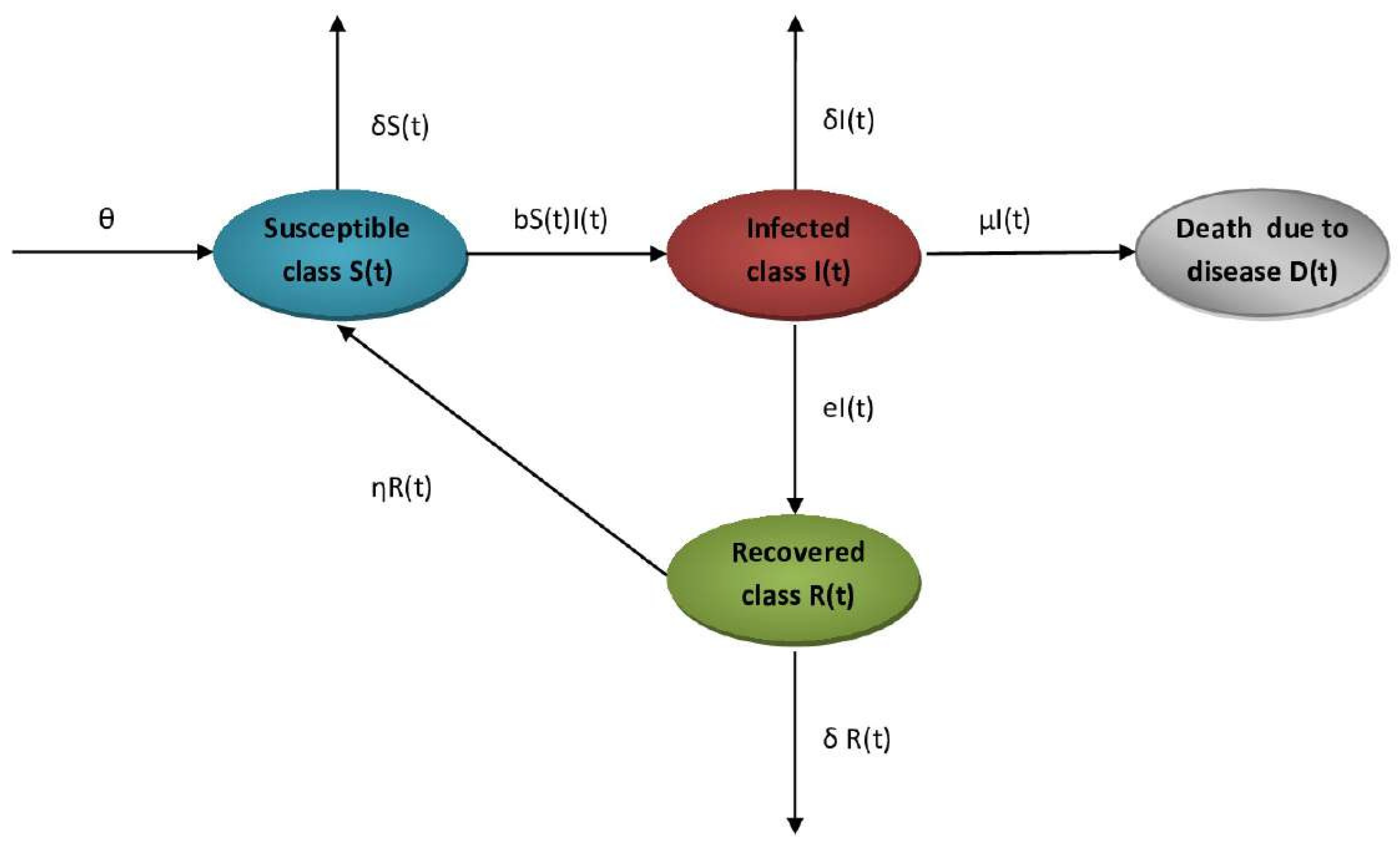
Figure 1. Disease transmission flow of the proposed model.
Mathematics 10 02224 g001
Figure 2. Numerical simulation of system (12).
Mathematics 10 02224 g002
Figure 3. Numerical simulation of infected class with integer and commensurate fractional-order and comparison with the real data.
Mathematics 10 02224 g003
Figure 4. Numerical simulation of system (56) with ( α 1 = 0.223 , α 2 = 0.2 , α 3 = 0.232 (56).
Mathematics 10 02224 g004
Figure 5. The comparison between the results of (56) and the real data.
Mathematics 10 02224 g005
Figure 6. The comparison between the integer order, the commensurate order, and the incommensurate order systems with the real data.
Mathematics 10 02224 g006
Table 1. Description of the model’s parameters.
ParametersDescription
μ Corona death rate
δ Natural death rate
θ The number of new births
bInfection rate
eRecovery rate
η The rate at which a recovering person is at risk of infection
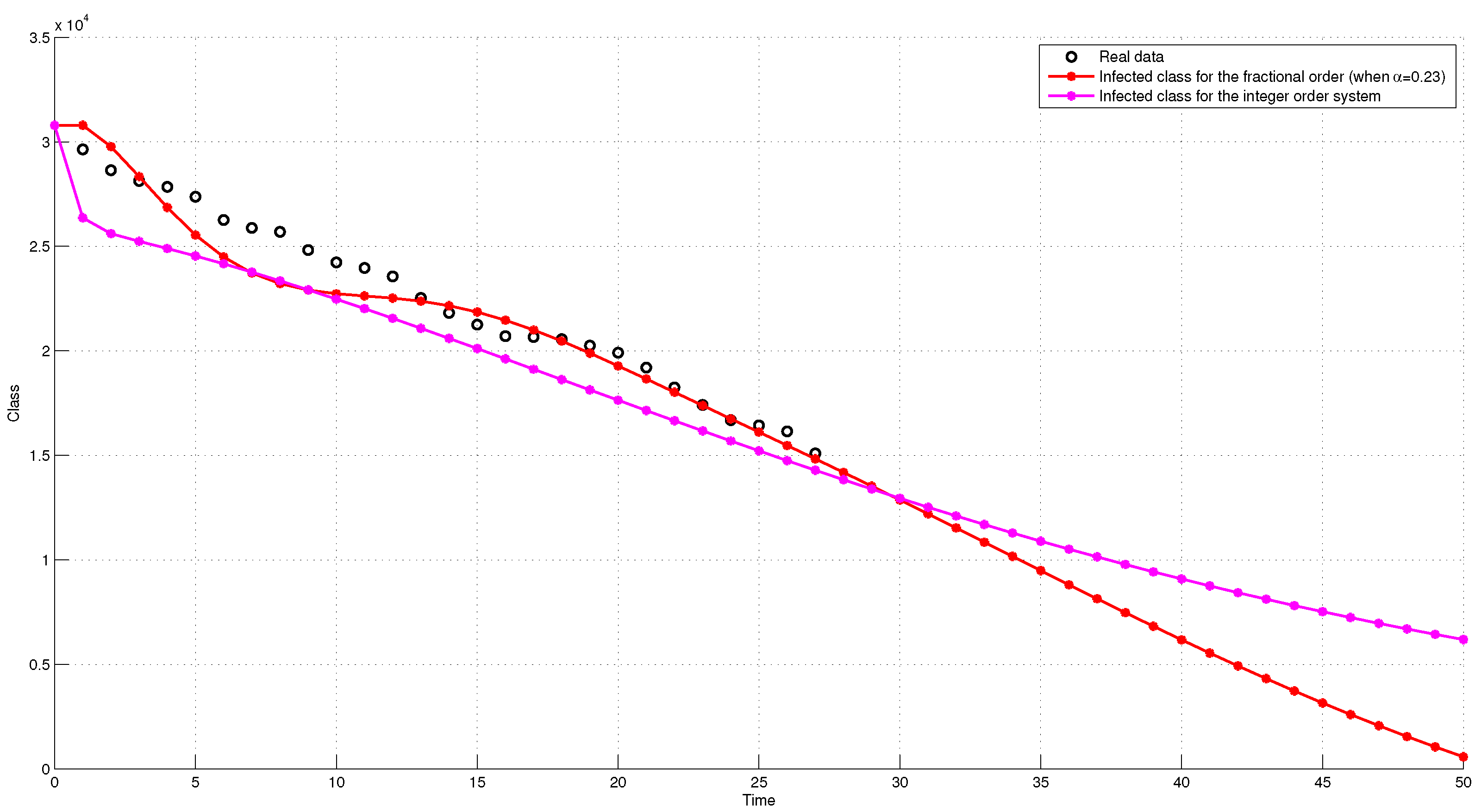
Table 2. Real data: The number of active infections in Germany in the period 26 April to 23 May 2020 [51].
26-Apr27-Apr28-Apr29-Apr30-Apr1-May2-May
30,79129,63728,64228,12627,84527,37526,262
3-May4-May5-May6-May7-May8-May9-May
25,88425,69324,82624,23423,96823,56522,531
10-May11-May12-May13-May14-May15-May16-May
21,81721,25320,70720,66420,55720,25019,914
17-May18-May19-May20-May21-May22-May23-May
19,20018,25417,41116,68716,43516,15115,092
Publisher’s Note: MDPI stays neutral with regard to jurisdictional claims in published maps and institutional affiliations.

