Multiple Scenarios of Quality of Life Index Using Fuzzy Linguistic Quantifiers: The Case of 85 Countries in Numbeo

Abstract

In economic development, in addition to comparing the gross domestic product (GDP) between nations, it is critical to assess the quality of life to gain a holistic perspective of their different aspects. However, the quality of life index (QOLI) is a subjective term that can be difficult to quantify. Although this composite index is typically calculated using universal weights proposed by experts to aggregate indicators, such as safety indexes, healthcare indexes, pollution indexes, and housing indicators, it is complicated to balance multiple dimensions whose weights are adjusted to account for different countries’ circumstances. Therefore, this paper aims to construct various scenarios of the QOLI, using linguistic quantifiers of the ordered weighted averaging (OWA) operator, and the 2-tuple linguistic model. Numbeo, one of the largest quality of life information databases, was used in this paper to estimate the QOLI in 85 countries. Uncertainty and sensitivity analyses were employed to assess the robustness of the QOLI. The results of the proposed model are compared with those obtained using the Numbeo formulation. The results show that the proposed model increases the linguistic interpretability of the QOLI, and obtains different QOLIs, based on diverse country contexts.

1. Introduction

The gross domestic product (GDP) of a country reflects economic growth, and GDP per capita has a strong relationship with the evolution of living standards over time. But GDP is not equal to well-being, as it does not include some factors that contribute to a good life. Quality of life (QOL) is a concept introduced to reflect a comprehensive view of many aspects of well-being in a country or a city. The measurement and study of QOL are increasingly significant in social development, as it encompasses many aspects, such as healthcare, housing costs, education, employment opportunities, etc.

However, QOL is a difficult concept to measure as it is multifaceted, interacts with a variety of living settings, and is influenced by people’s lifestyles and preferences. In many studies [1,2,3,4,5,6,7,8,9,10], QOL is considered a subjective term to describe people’s well-being in their countries. In the literature, QOL is defined in various ways [11,12,13,14,15].

The Quality of Life Index (QOLI), developed by the World Health Organization (WHO), and the Better Life Index (BLI), developed by the Organization for Economic Co-operation and Development (OECD), are two typical indices for measuring the quality of life in various nations. Both are determined by considering variables such as housing indicators, environmental issues, safety indexes, and healthcare indexes, among others.

The QOLI can be considered a composite indicator, as it aggregates separate metrics to reflect the overall quality of life of a country or city. To obtain this composite indicator to compare the quality of life in different countries, many experts propose using universal weights. Nevertheless, this index is a complex balance of multiple factors, the weights of which should vary according to the circumstances of each country. For instance, the weight distribution of various indicators should be different in emerging and developed countries.

Therefore, the purpose of this paper is to construct various scenarios of QOLI using linguistic quantifiers of the ordered weighted averaging (OWA) operator, and the 2-tuple linguistic model. The advantage of employing the 2-tuple linguistic model in the proposed model is that it allows aggregating the information without information distortion and loss, as well as improving the understandability and intuitiveness of its outcomes presented in linguistic terms [16]. Numerical values need to be sorted to determine their low or high level, but linguistic terms can be comprehended directly by people without needing for further comparison. The advantage of using linguistic terms is that it directly shows whether the QOLI is very low, low, moderate, high, or very high, even when the data for the different sub-indicators are not on the same scale.

In summary, the contribution of this proposed model is to use the OWA operator and 2-tuple linguistic model to form the 2-tuple linguistic ordered weighted averaging (2LOWA) operator. The novelties of this model in the construction of the QOLI are that it can not only adjust the weights used by Numbeo’s experts to obtain many QOLI scores considering country-specific situations, but it also can convert the numbers into linguistic scales that are easily understandable and interpretable by humans. The data used to verify the applicability of the proposed model came from Numbeo, one of the largest databases of quality of life information. The results show that this model enables assigning different weights to each dimension to generate more QOLI scores, and produces the same QOLI as the model using the weights proposed by experts. Moreover, it aggregates numerous indicators to a 2-tuple value, reducing information loss and improving the linguistic interpretability of the QOLI.

The rest of this paper is organized as follows. In Section 2, the essential concepts on which the proposed model is based are introduced. In Section 3, the proposed methodology to obtain more scenarios for the QOLI computation is presented. In Section 4, the results of the QOLI obtained by the proposed model for 85 countries are analyzed and compared. In Section 5, the advantages and shortcomings of the proposed model are discussed, including its validation by uncertainty and sensitivity analysis. In Section 6, the conclusions and future work are described.

2. Theoretical Framework

2.1. Composite Indicators

Composite indicators can summarize the information contained in several sub-indicators or variables, which is more accessible than attempting to discover a common trend in various sub-indicators [17]. They are generally used to identify competitiveness, innovation capacity, and sustainable development of countries or companies; some examples are the Human Development Index (HDI), the Environmental Performance Index (EPI), the Air Quality Index (AQI), the Quality of Life Index (QOLI), the Corruption Perceptions Index (CPI), and the Globalization Index (GI). For composite indicators, a framework is always necessary to determine which variables to include and their corresponding weights. When creating composite indicators, one of the crucial steps is how to weight the sub-indicators [18]. Weighting the sub-indicators leads to the last step in building composite indicators: aggregation.

There are a variety of aggregation methods for building composite indicators. For substitutable sub-indicators or variables, one of the most commonly used aggregation methods is principal component analysis (PCA) [19], as it can handle high dimensional data [20] by summarizing them in fewer dimensions while keeping the maximum proportion of the original data variance [21].

For non-substitutable sub-indicators or variables, non-linear approaches are employed, such as non-compensatory multi-criteria analysis, or multiplicative functions (partially compensatory approach) [22]. Indeed, multi-criteria decision-making (MCDM) approaches are frequently utilized to create composite indicators, because they are ideal for converting multiple sub-indicators into a composite indicator [23].

Table 1. MCDM methods for the construction of composite indicators.

Method	Description	Literature	Application
Analytic hierarchy process (AHP)	A method for measuring the weights of structure components by using a paired comparison scale.	Saaty, 1987 [24]	Composite cyclical-performance index [25], environmental sustainability index [26], agricultural sustainability index [27]
Analytic network process (ANP)	An extension of the AHP that allows for interdependencies between criteria.	Saaty, 1996 [28]	Disaster resilience indicator [29], ecological water quality index [30]
Criteria importance through intercriteria correlation (CRITIC)	A method for determining objective weights for each criterion by employing correlation analysis between criteria.	Diakoulaki et al., 1995 [31]	Energy security index [32]
Data envelopment analysis (DEA)	A non-parametric method for measuring the efficiency of a group of multiple decision-making units, with multiple inputs and outputs.	Charnes et al., 1978 [33]	Spanish public university quality index [34], sustainability index [35]
Elimination et choix traduisant la realité (ELECTRE)	A method for determining the concordance and discordance indices of a group of alternatives, and ranking them from best to worst.	Roy, 1968 [36]	Human development index [37], land-use policy efficiency index [38]
Preference Ranking Organization Method for Enrichment Evaluation (PROMETHEE)	A method for producing a ranking based on choosing a preference function for each criterion in an MCDM issue.	Brans and Vincke, 1985 [39]	European countries sustainability index [40]
Simple Additive Weighting (SAW)	A method for calculating a weighted score for each alternative by multiplying each attribute’s contributions by their weights.	Churchman and Ackoff, 1954 [41]	Neighborhood sustainability index [42]
Technique for Order of Preference by Similarity to Ideal Solution (TOPSIS)	A compensatory aggregation method for choosing between the shortest Euclidean distance to the ideal solution, and the biggest distance to the negative ideal solution.	Hwang and Yoon, 1981 [43]	Road safety performance index [44], financial and diversity performance index [45], clean energy index [46]
Ordered weighted averaging (OWA)	A symmetric aggregation method for distributing weights based on the input value and unifies multiple inputs in one operator.	Yager, 1988 [47]	Energy supply security index [48], disaster resilience index [49]
Visekriterijumska Optimizacija I kompromisno resenje (VIKOR)	A method for calculating the compromise ranking list of a group of alternatives, based on the measure of closeness to the ideal option.	Duckstein and Opricovic, 1980 [50]	Academic performance index [51]
Benefit of the doubt (BoD)	A method derived from the DEA, which is a linear mathematical programming methodology, to assign the most favorable weight for each observation. These weights enable both data normalization and objective weighing.	Melyn and Moesen, 1991 [52]	Digital access index [53], human development index [54,55], non-parametric corporate social responsibility index [56]

demonstrates several MCDM approaches to constructing composite indicators, and some examples of their application, each with distinct weight distribution.

MCDM approaches can be divided into compensatory and non-compensatory approaches [57,58]. Compensation refers to compensating a ‘disadvantage’ of some attribute with a sufficiently large ‘advantage’ of another, whereas it would not be possible to do so with lesser ‘advantages’ [59,60]. The compensatory aggregation-based MCDM methods include AHP, SAW, and TOPSIS. Non-compensatory means that a decision determined by some attributes cannot be altered by others [61]. Non-compensatory approaches include preference aggregation-based methods (e.g., ELECTRE, PROMETHEE, etc.) and rules-based methods [62]. This type of aggregation method speeds up and facilitates decision-making. However, non-compensatory approaches do not consider all relevant data, and often overlook the relative importance of certain attributes [61].

In addition to recognizing the characteristics of various models to construct composite indicators, it is necessary to verify the robustness of the composite indicator. The changeability in the weights, and the imputation of missing data, contribute to the uncertainty in the calculation of composite indicators [21]. If composite indicators are poorly constructed, they may convey misleading messages.

In the literature, sensitivity analysis is often applied to investigate the robustness of the ranking of the weights of multiple criteria in the MCDM process [63,64,65]. Alexander’s A indicator (AAI) [66], one of the sensitivity indicators, is utilized to quantify the degree of change in the rankings of these indicators, where 0 represents no change, and 1 represents a complete reversal in ranks. The robustness of composite indicators can be assessed by uncertainty analysis and sensitivity analysis [67]. Uncertainty analysis measures the fluctuations in the result (i.e., the value of the composite indicators) derived from the uncertainty in the input factors (i.e., the construction stages of composite indicators: selection of aggregation approaches, weights of the sub-indicators, etc.) [68,69]. The sensitivity analysis determines how much of the overall output variation is attributable to such uncertainties [67].

The robustness of the composite indicator ranking can be assessed by a combination of uncertainty and sensitivity analysis [70]. The rank assigned by the composite indicator to each country is an output of the uncertainty and sensitivity analysis [70]. It can be used to determine the average change in country ranking and assess the quality of the composite indicator. Its definition is as follows:

Definition 1.

The average of the absolute differences in country rankings [67,70] is shown in Formula (1):

$$\overline{R_s}=\frac{1}{M}{\displaystyle \sum _{c=1}^M\left|ran{k}_{ref}(C{I}_c)-ran{k}_q(C{I}_c)\right|}$$

(1)

where M is the number of countries; $ran{k}_{ref}\left(C{I}_c\right)$ represents the reference ranking of each country (in this paper, it is the actual rank of each country’s quality of life index on Numbeo); and $ran{k}_q\left(C{I}_c\right)$. represents the ranking assigned to each country based on the quality of life index calculated by diverse quantifiers.

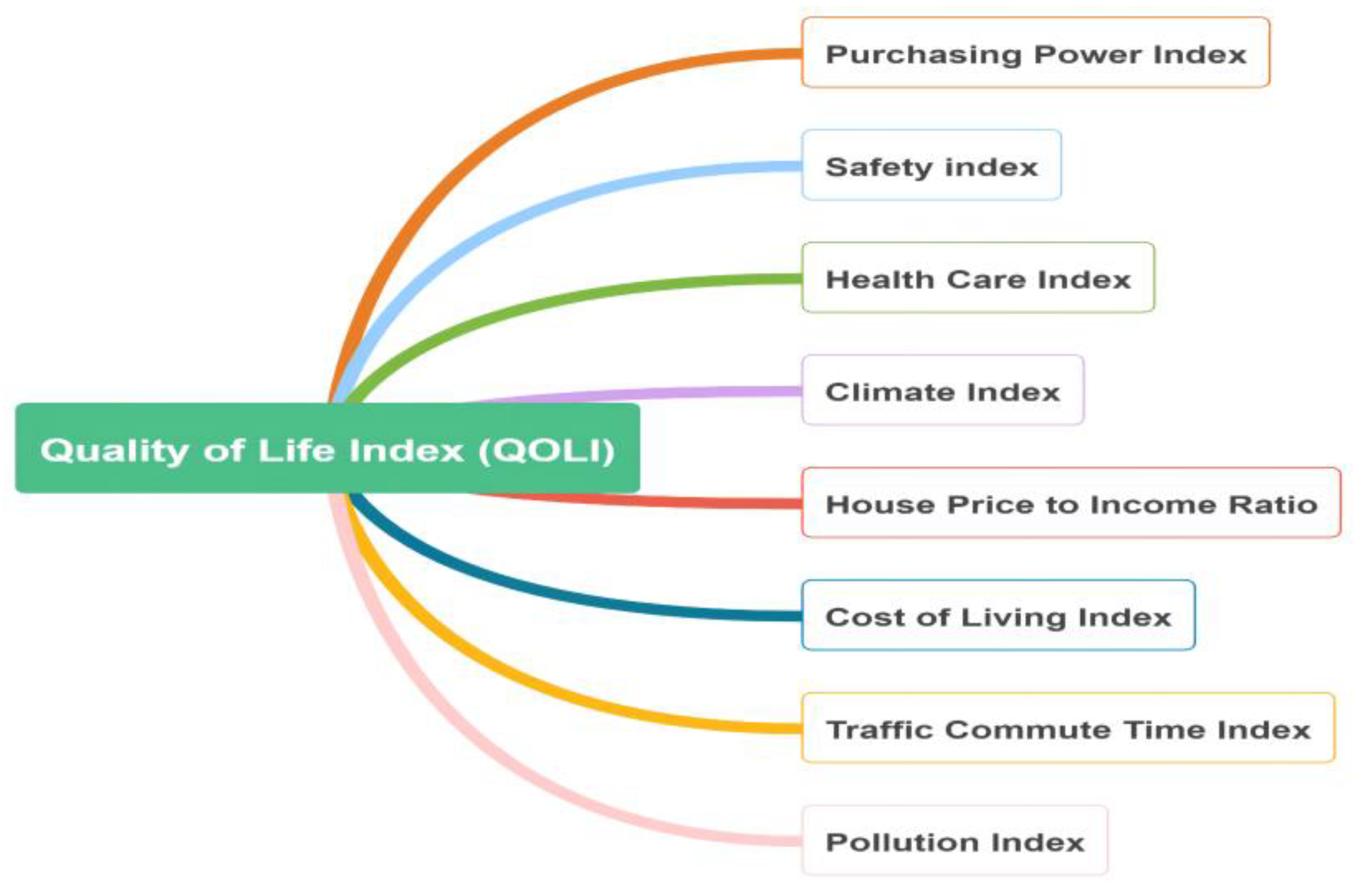
2.2. The Quality of Life Index

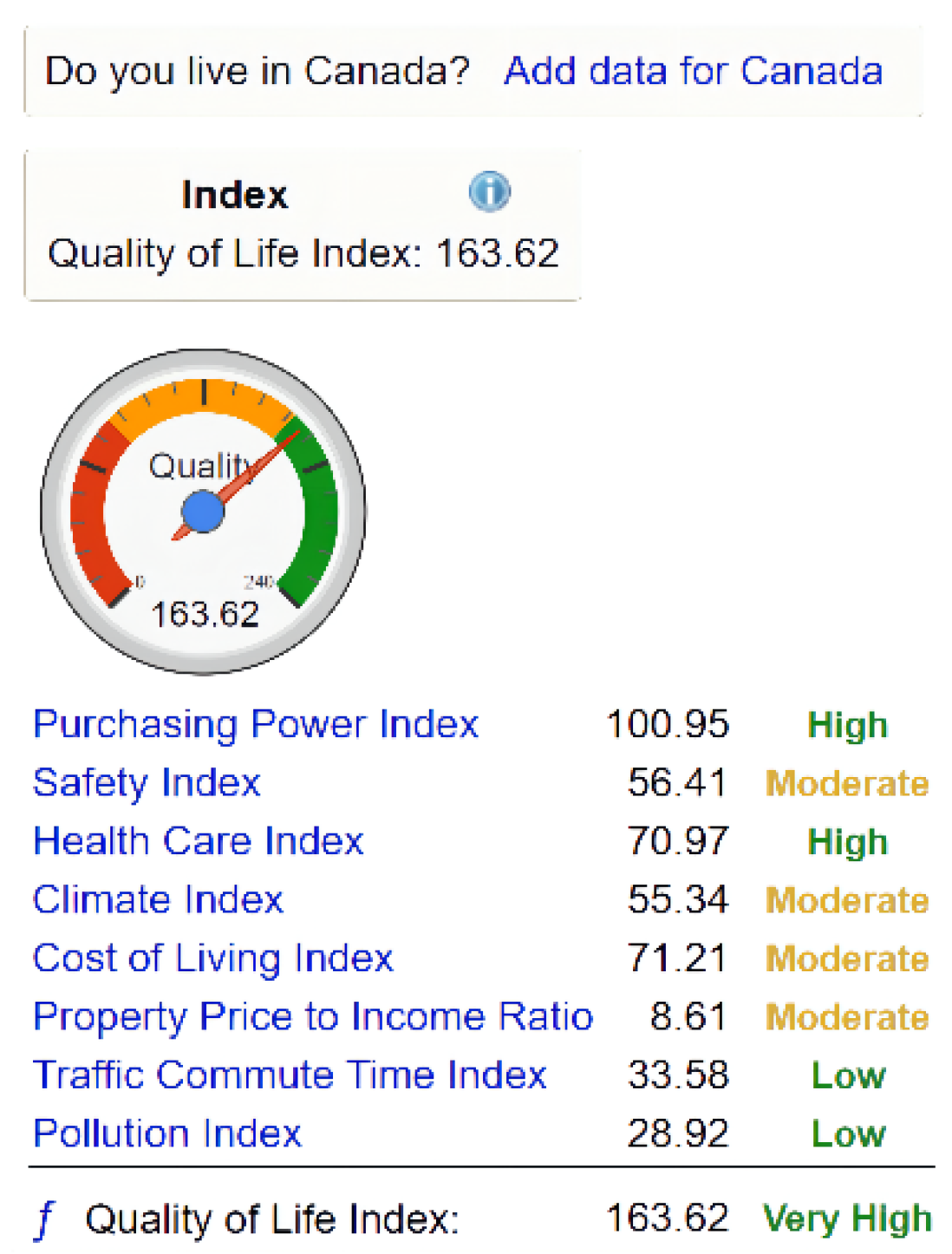
The QOL is a complex term that can be defined in various ways in different disciplines, such as medicine, international development, and politics, so it does not have a commonly accepted definition. The WHO defines it as a person’s perception of his or her position in life in the context of the culture and value systems in which he or she lives, and in relation to his or her goals, expectations, standards, and concerns [71]. Therefore, the QOL combines a person’s assessment of numerous dimensions of safety, education, medical and healthcare services, and other aspects of life that cannot be easily equated with terms such as “life satisfaction”, “happiness”, or “income level”.

Many researchers and institutions, such as Eurostat, WHO, and WorldData, among others, have attempted to measure the QOL using the quality of life index (QOLI). Numbeo, one of the world’s largest databases of quality of life information, has been developing and improving its algorithm for calculating the QOLI. The factors that Numbeo takes into account in calculating the QOLI are listed below (see also Figure 1):

• Purchasing power index (${\mathrm{I}}_{\mathrm{purchasing}\text{\_}\mathrm{p}}$, including rent index): a relative purchasing power in buying goods and services in a given city or country for the average net salary;
• Safety index (${\mathrm{I}}_{\mathrm{safety}}$): an indicator taking into account concerns about robberies, vehicle theft, and other crimes, as well as the incidence of narcotics, property crime, violent crime, and corruption and bribery. This index is the opposite of the crime index;
• Health care index (${\mathrm{I}}_{\mathrm{health}\text{\_}\mathrm{c}}$): an estimation of the overall quality of the health care system, health care professionals, equipment, staff, doctors, cost, etc.;
• Climate index (${\mathrm{I}}_{\mathrm{climate}}$): an estimation of the climate likability of a given city or a country;
• House price to income ratio (${\mathrm{I}}_{\mathrm{house}\text{\_}\mathrm{p}}$): the basic measure for apartment purchase affordability. It is calculated as the ratio of median apartment prices to median familial disposable income, expressed as years of income;
• Cost of living index (${\mathrm{I}}_{\mathrm{cost}\text{\_}\mathrm{liv}}$, excluding rent index): a relative indicator of consumer goods prices, including groceries, restaurants, transportation, and utilities. This index does not include accommodation expenses such as mortgage or rent;
• Traffic commute time index (${\mathrm{I}}_{\mathrm{traffic}\text{\_}\mathrm{t}}$): a composite index of time consumed in traffic due to job commute, estimation of time consumption dissatisfaction, estimation of CO₂ consumption in traffic, and overall inefficiencies in the traffic system;
• Pollution index (${\mathrm{I}}_{\mathrm{pollution}}$): an estimation of the overall pollution in a given city or a country, taking into account air pollution, water pollution, and other pollution types.

Definition 2.

The current formula applied by Numbeo [72] is shown in Formula (2):

$$\begin{array}{l}\mathrm{QOLI}=100+\frac{{\mathrm{I}}_{\mathrm{purchasing}\text{\_}\mathrm{p}}}{2.5}+\frac{{\mathrm{I}}_{\mathrm{safety}}}{2}+\frac{{\mathrm{I}}_{\mathrm{health}\text{\_}\mathrm{c}}}{2.5}+\frac{{\mathrm{I}}_{\mathrm{climate}}}{3}-{\mathrm{I}}_{\mathrm{house}\text{\_}\mathrm{p}}-\frac{{\mathrm{I}}_{\mathrm{cost}\text{\_}\mathrm{liv}}}{10}-\frac{{\mathrm{I}}_{\mathrm{traffic}\text{\_}\mathrm{t}}}{2}-\frac{2\cdot {\mathrm{I}}_{\mathrm{pollution}}}{3}\\ \hspace{1em}\hspace{1em} =100+3.9\cdot (10.26\%\cdot {\mathrm{I}}_{\mathrm{purchasing}\text{\_}\mathrm{p}}+12.82\%\cdot {\mathrm{I}}_{\mathrm{safety}}+10.26\%\cdot {\mathrm{I}}_{\mathrm{health}\text{\_}c}+8.55\%\cdot {\mathrm{I}}_{\mathrm{climate}}\\ \hspace{1em}\hspace{1em}\hspace{1em}\hspace{1em}\hspace{1em}\hspace{1em}\hspace{1em}\hspace{1em}-25.64\%\cdot {\mathrm{I}}_{\mathrm{house}\text{\_}\mathrm{p}}-2.56\%\cdot {\mathrm{I}}_{\mathrm{cost}\text{\_}\mathrm{liv}}-12.82\%\cdot {\mathrm{I}}_{\mathrm{traffic}\text{\_}\mathrm{t}}-17.09\%\cdot {\mathrm{I}}_{\mathrm{pollution}})\end{array}$$

(2)

Among these eight sub-indicators, the larger the value of the four sub-indicators—purchasing power index, safety index, health care index, and climate index—the better. The smaller the rest of the sub-indicators, the better.

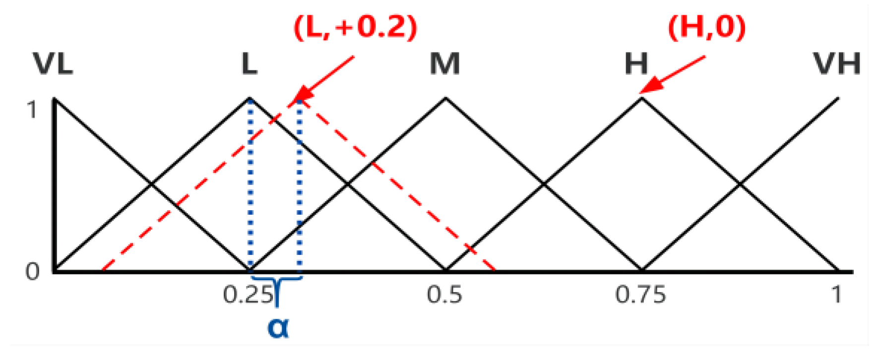
2.3. The 2-Tuple Linguistic Model

The 2-tuple linguistic model introduced by Herrera and Martínezin has a continuous and ordinal scale, in order to avoid information loss in the fusion of linguistic information [73], which provides linguistically accurate and more understandable results. Based on the concept of symbolic translation, this model represents the linguistic information by a 2-tuple value $\left(s_i,\alpha \right)$, where $s_i\in S$ is a linguistic term, and $\alpha \in \left[-0.5,0.5\right)$ is a numerical value representing the distance to the central value of $s_i$. $S=\left\{s_0=Very Low=VL, s_1=Low=L, s_2=Moderate=M, s_3=High=H, s_4=Very High=VH\right\}$ is a set of five linguistic terms used in the Numbeo database, whose definition is shown in Figure 2.

Definition 3.

Let $S=\left\{s_0,\dots ,s_g\right\}$ be a set of linguistic terms, whose cardinality is  $g+1$. $\beta \in \left[0,g\right]$ is a value that supports the outcome of a symbolic aggregation operation. The function $\Delta :\left[0, g\right] \to S=Sx\left[-0.5,0.5\right)$ is used to convert β to 2-tuple value  $\left(s_i,\alpha \right)$ as shown in Formula (3):

$$\Delta \left(\beta \right)=\left(s_i,\alpha \right),with\{\begin{array}{l}i=round(\beta )\\ \alpha =\beta -i, \alpha \in [-0.5,0.5)\end{array}$$

(3)

where round(·) is the rounding operation; $s_i$ is the index of the label nearest to β; and α is a numerical value representing the symbolic translation. Note that the function $\Delta$ is bijective, so the function ${\Delta }^{-1}: S=Sx\left[-0.5,0.5\right) \to \left[0, g\right]$ can be used to return an equivalent numerical value β as ${\Delta }^{-1}\left(s_i,\alpha \right)=i+\alpha =\beta$.

The following is an example of a transformation from a numerical value to a 2-tuple value, as well as a retranslation from a 2-tuple value to a numerical value.

Assume that β = 1.2 is a value representing the result of a symbolic aggregation operation on the set of linguistic terms $S=\left\{s_0=VL,s_1=L,s_2=M,s_3=H,s_4=VH\right\}$, whose 2-tuple value is calculated as $\Delta \left(1.2\right)=\left(s_{round\left(1.2\right)},1.2-s_{round\left(1.2\right)}\right)=\left(s_1,+0.2\right)=\left(L,+0.2\right)$. Its numerical transformation is performed by the function ${\Delta }^{-1}$, that is ${\Delta }^{-1}\left({\mathrm{s}}_1,+0.2\right)$ = $1+0.2=1.2$. If β is equal to 3, its 2-tuple value is $\Delta \left(3\right)=\left(s_3,0\right)=\left(H,0\right)$, which means that the difference between β and this linguistic term is 0 (α = 0). Note that adding the value zero as a symbolic translation, $s_i\in S\to \left(s_i,0\right)$, is identical to the label without symbolic translation $\left(H,0\right)=H$. Figure 3 shows the two examples mentioned above.

The negation operator and a comparison between two linguistic 2-tuple values were also introduced in the 2-tuple linguistic model as follows:

Definition 4.

The negation operator of a 2-tuple value is defined as Formula (4):

$$neg\left((s_i,\alpha )\right)=\Delta (g-({\Delta }^{-1}(s_i,\alpha )))=\Delta (g-\beta )$$

(4)

Definition 5.

The comparison of linguistic information represented by 2-tuple values is performed according to a lexicographic order. Let $\left(s_G,{\alpha }_1\right)$ and $\left(s_M,{\alpha }_2\right)$ be two 2-tuple values, so that their linguistic 2-tuple values are compared as follows:

• If G < M, $\left(s_G,{\alpha }_1\right)$ is smaller than $\left(s_M,{\alpha }_2\right)$;
• If G = M, when:
  • ${\alpha }_1={\alpha }_2$, $\left(s_G,{\alpha }_1\right)$ is the same as $\left(s_M,{\alpha }_2\right)$;
  • ${\alpha }_1<{\alpha }_2$, $\left(s_G,{\alpha }_1\right)$ is smaller than $\left(s_M,{\alpha }_2\right)$;
  • ${\alpha }_1>{\alpha }_2$, $\left(s_G,{\alpha }_1\right)$ is larger than $\left(s_M,{\alpha }_2\right)$;
• If G > M, $\left(s_G,{\alpha }_1\right)$ is larger than $\left(s_M,{\alpha }_2\right)$.

2.4. The Ordered Weighted Averaging (OWA) Operator

Yager introduced the concept of the OWA operator in 1988 to solve the MCDM problems, and to generate an overall decision function [47].

Definition 6.

An OWA operator of dimension n is a mapping of $OWA: R^n\to R$, with an associated weighting vector W of dimension n, such that ${\displaystyle \sum }_{i=1}^n{w}_i=1$ and $w_i\in \left[0, 1\right]$. Thus, the OWA for each linguistic quantifier is calculated using Formula (5):

$$OWA(a_1,a_2,\dots a_n)={\displaystyle \sum _{i=1}^n{w}_i{b}_i}$$

(5)

where $a_1,a_2, \dots , a_n$ are the input values; $b_i$ is the ith largest element of the input values; and $w_i$ represents the ordered weights.

The ordered weights $w_i$ ($w_i\in \left[0, 1\right]$) are always calculated according to the linguistic quantifiers (At least one, Some, Half, Most, All, etc.) because they express different degrees of demand in natural language by using formal mathematical formulas [74]. The complementary values orness and tradeoff are computed from these quantifiers to represent the degree of optimism, or different attitudes toward risk, while making decisions.

In fact, compared with other approaches (see Table 1) used to generate composite indicators, using linguistic quantifiers, the OWA operator can aggregate the information to make a compensation levels regulation between variables [75]. The OWA operator can be used to reflect compensatory and non-compensatory preferences. This attribute is expressed by the degree of orness of an OWA operator [47]. As each linguistic quantifier is associated with a particular value, the OWA operator can be used to express the attitudinal character of the decision-maker in the information aggregation [76]. It means that, with the application of different linguistic quantifiers, numerous scenarios that consider different country circumstances can be obtained from the initial weights supplied by the experts. Furthermore, the OWA operator solves non-compensatory aggregation issues [61], resulting in a statistically consistent composite indicator [77].

Definition 7.

Regular increasing monotone (RIM) quantifiers can be applied to generate a parameterized subset in the unit interval [78], as shown in Formula (6):

$$Q(p)=p^{\lambda }, \lambda >0$$

(6)

where $Q$ is a linguistic quantifier, represented as a fuzzy subset over the unit interval [0, 1]; for each p in the unit interval, the grade of membership $Q\left(p\right)$ indicates the compatibility of p with the concept denoted by $Q$.

Table 2. Linguistic quantifiers with their associated parameters $\lambda$.

Linguistic Quantifier	$\mathit{\lambda }$
At least one	0.0001
Few	0.1
Some	0.5
Half	1
Many	2
Most	10
All	1000

shows the parameter $\lambda$ proposed by [79] for each linguistic quantifier.

Definition 8.

The ordered weights $w_i$ ($w_i\in \left[0, 1\right]$) are calculated using Formula (7):

$$w_i=Q(\frac{i}{n})-Q(\frac{i-1}{n})={(\frac{i}{n})}^{\lambda }-{(\frac{i-1}{n})}^{\lambda },\lambda >0,i=1,\dots ,n$$

(7)

where n is the number of criteria or sub-indicators $i=1$,…, n, and $\lambda$ is the value related to each linguistic quantifier $Q$. The larger $\lambda$ is, the less risky the decision is. $\lambda$ = 1 represents a moderate degree of risk.

Definition 9.

Related to the ordered weights, orness and tradeoff represent different attitudes toward risk while making decisions. Orness shows the level of risk in the aggregation process, while the tradeoff is its compensation. They can be calculated as shown in Formulas (8) and (9) [47,80]:

$$orness(w)=\frac{1}{n-1}{\displaystyle \sum _{i=1}^n(n-i)}\ast w_i,i=1,\dots ,n$$

(8)

$$tradeoff(w)=1-\sqrt{\frac{n{\displaystyle \sum _{i=1}^n(w_i-\frac{1}{n}{)}^2}}{n-1}}$$

(9)

If the quantifier At least one is employed to calculate the ordered weights, orness is one and tradeoff zero, representing the maximum risk. When orness and tradeoff equal zero, using the quantifier All, the minimum risk is attained. If the quantifier Half is used, orness equaling 0.5 and tradeoff equaling 1 represents the medium risk.

2.5. The 2-Tuple Linguistic Ordered Weighted Averaging (2LOWA) Operator

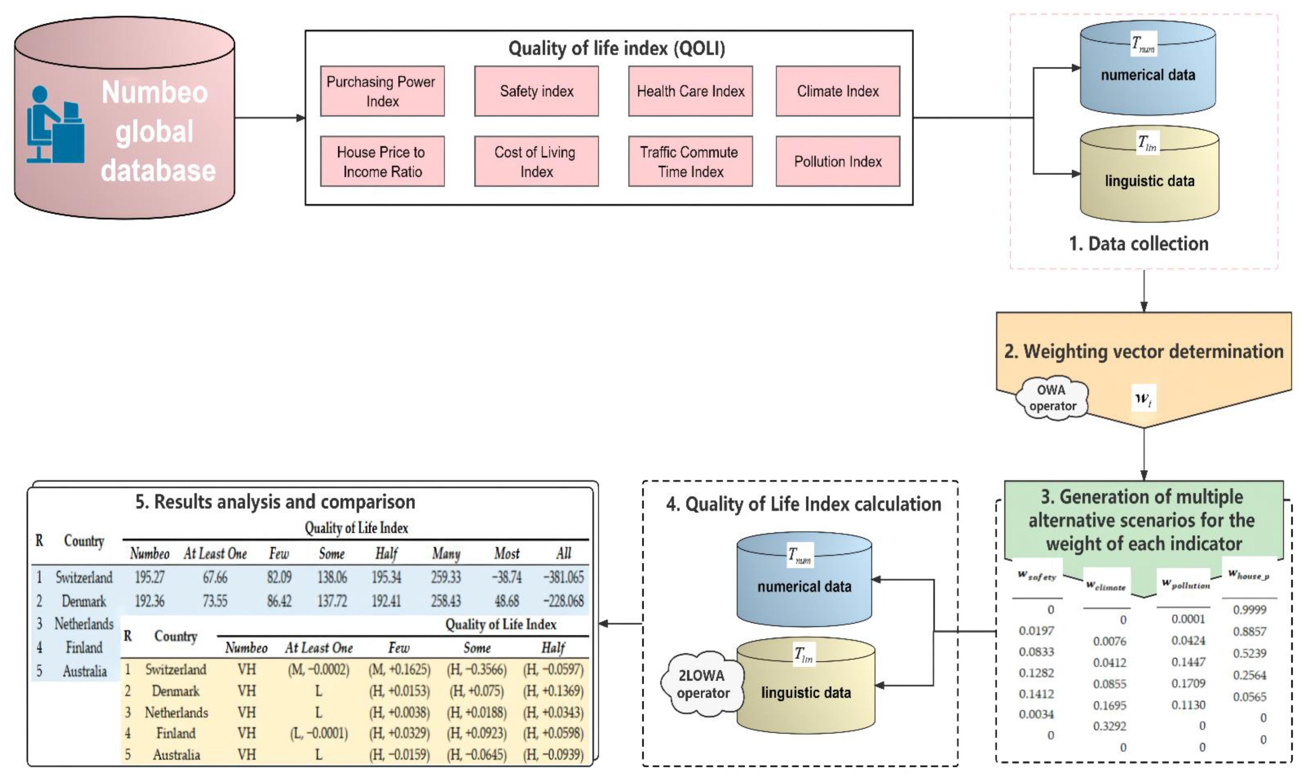
The 2-tuple linguistic ordered weighted averaging (2LOWA) operator is an extension of the OWA operator that uses linguistic information expressed in 2-tuple values. It is particularly effective when the decision-maker cannot analyze the information only based on numerical scales, but also requires a linguistic interpretation. The definition is as follows.

Definition 10.

A 2LOWA operator of dimension n is a mapping of 2LOWA: $R^n\to R$, with an associated weighting vector W of dimension n, such that ${\displaystyle \sum }_{i=1}^n{w}_i=1$ and $w_i\in \left[0, 1\right]$. The function $\Delta :\left[0, g\right] \to S$ is used to convert numerical values into 2-tuple values, as shown in Formula (10):

$$2LOWA((s_1,{\alpha }_1),\dots ,(s_n,{\alpha }_n))=\Delta \left({\displaystyle \sum _{i=1}^n{w}_i{b}_i}\right)$$

(10)

where $\left\{\left(s_1,{\alpha }_1\right),\dots ,\left(s_n,{\alpha }_n\right)\right\}$ is the set of 2-tuple values; $w_i$ represents the ordered weights; and $b_i={\mathsf{\Delta }}^{-1}\left(s_i,{\alpha }_i\right)$.

3. Methodology

This section demonstrates the procedure for acquiring alternative scenarios about the quality of life index, based on the 2LOWA–QOLI model. This model is shown in Figure 4, which includes the following five steps:

• Step 1. Data collection.

The purpose of this step was to obtain information about the quality of life in 85 countries from Numbeo. This database [81] contains current data on global living conditions, given by millions of people worldwide. It provides data ranging from pollution levels to information on traffic, the health system, safety, and property prices. For information about the QOLI and its sub-indicators, Numbeo uses both numbers and linguistic quantifiers to express them. Figure 5 shows an example [82].

Let $C=\left\{c_1,\dots ,c_{\#C}\right\}$ be a set of countries obtained from Numbeo database [81]. As Numbeo uses numbers and a linguistic scale to express the degree of the quality of life in different countries, two datasets were obtained in this step: one for numerical calculations ($T_{num}$), and the other for linguistic terms ($T_{lin}$). For each dataset, the eight sub-indicators used in Numbeo to generate the QOLI were analyzed: the purchasing power index (${\mathrm{I}}_{\mathrm{purchasing}\text{\_}\mathrm{p}}$), the safety index (${\mathrm{I}}_{\mathrm{safety}}$), the health care index (${\mathrm{I}}_{\mathrm{health}\text{\_}\mathrm{c}}$), the climate index (${\mathrm{I}}_{\mathrm{climate}}$), the house price to income ratio (${\mathrm{I}}_{\mathrm{house}\text{\_}\mathrm{p}}$), the cost of living index (${\mathrm{I}}_{\cos \mathrm{t}\text{\_}\mathrm{liv}}$), the traffic commute time index (${\mathrm{I}}_{\mathrm{traffic}\text{\_}\mathrm{t}}$), and the pollution index (${\mathrm{I}}_{\mathrm{pollution}}$).

Let $T_{num}=\left\{\begin{array}{c}(c_1,\{v_{num}({\mathrm{I}}_{\mathrm{purchasing}\text{\_}\mathrm{p}}^{c_1}),\dots , v_{num}({\mathrm{I}}_{\text{pollution}}^{c_1})\})\\ ,\dots ,\\ (c_{\#T_{num}},\{v_{num}({\mathrm{I}}_{\mathrm{purchasing}\text{\_}\mathrm{p}}^{c_{\#T_{num}}}),\dots , v_{num}({\mathrm{I}}_{\text{pollution}}^{c_{\#T_{num}}})\})\end{array}\right\}$ be the numerical data for these eight sub-indicators from 85 different countries, and $T_{lin}=\left\{\begin{array}{c}(c_1,\{v_{lin}({\mathrm{I}}_{\mathrm{purchasing}\text{\_}\mathrm{p}}^{c_1}),\dots ,v_{lin}({\mathrm{I}}_{\mathrm{pollution}}^{c_1})\})\\ ,\dots ,\\ (c_{\#T_{lin}},\{v_{lin}({\mathrm{I}}_{\mathrm{purchasing}\text{\_}\mathrm{p}}^{c_{\#T_{lin}}}),\dots , v_{lin}({\mathrm{I}}_{\mathrm{pollution}}^{c_{\#T_{lin}}})\})\end{array}\right\}$ be their linguistic data, where:

• $c_r$ is the name of each country, with $c_r\in C$, and $r=1,\dots ,\#C$;
• $\{v_{num}({\mathrm{I}}_{\mathrm{purchasing}\text{\_}\mathrm{p}}^{c_r}),\dots , v_{num}({\mathrm{I}}_{\mathrm{pollution}}^{c_r})\}$ are the numerical values of eight sub-indicators for each country;
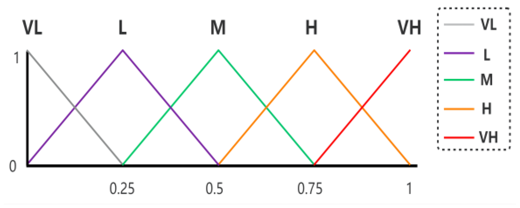
• $\{v_{lin}({\mathrm{I}}_{\mathrm{purchasing}\text{\_}\mathrm{p}}^{c_r}),\dots , v_{lin}({\mathrm{I}}_{\mathrm{pollution}}^{c_r})\}$ are the 2-tuple values of eight sub-indicators for each country, expressed on a linguistic scale. Based on Numbeo, this linguistic scale contains five values: “Very Low”, “Low”, “Moderate”, “High”, and “Very High”. These linguistic values are symmetrical, whose center value is neutral (i.e., “Moderate”) [83,84,85]. They can be modeled by fuzzy triangular labels, as shown in Figure 2.

• Step 2. Weighting vector determination.

This step was to establish the weighting vector for each linguistic quantifier, whose results are shown in

Table 3. Weighting vector for each linguistic quantifier.

Linguistic Quantifier	Weighting Vector
At least one	0.9998	0.0001	0	0	0	0
Few	0.8360	0.06	0.0371	0.0272	0.0217	0.0181
Some	0.4082	0.1691	0.1298	0.1094	0.0964	0.0871
Half	0.1667	0.1667	0.1667	0.1667	0.1667	0.1667
Many	0.0278	0.0833	0.1389	0.1944	0.2500	0.3056
Most	0	0	0.0010	0.0164	0.1442	0.8385
All	0	0	0	0	0	1

. These values are determined based on Formula (7).

The following is an example of how to calculate the weights for the quantifier At least one ($\alpha =0.0001$), and $n=6$, as several indicators should have the same weight, although Numbeo uses eight sub-indicators to calculate the quality of life [72,86,87]

$$\begin{gathered} w_i=Q(\frac{i}{6})-Q(\frac{i-1}{6})=(\frac{i}{6}{)}^{0.0001}-(\frac{i-1}{6}{)}^{0.0001}, i=1,\dots ,6 \\ {w}_i=(0.9998, 0.0001, 0, 0, 0, 0) \end{gathered}$$

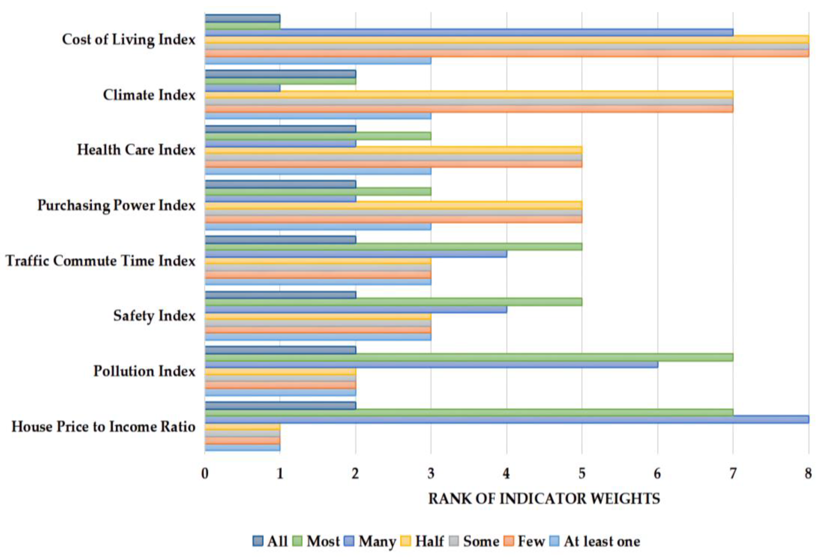
• Step 3. Generation of multiple alternative scenarios for the weight of each indicator.

Let v = (0.2564, 0.1709, 0.1282, 0.1282, 0.1026, 0.1026, 0.0855, 0.0256) be the vector that represents the weight of each indicator given by Numbeo’s experts in the calculation of the QOLI [72], corresponding to the indicators of house price to income ratio, the pollution index, the safety index, the traffic commute time index, the purchasing power index, the health care index, the climate index, and the cost of living index, respectively.

Since the QOLI is a subjective term that is a complicated balance of numerous sub-indicators, whose weights should differ depending on the country’s circumstances, this step aimed to obtain different alternative scenarios for the weight of each sub-indicator, by using various linguistic quantifiers. Therefore, based on the approach for calculating weights introduced by [88], the vector v was recalculated by multiplying it with the weighting vector of each linguistic quantifier (see Table 3).

Table 4. Results of the recalculated weights for each indicator.

Linguistic Quantifier	whouse_p	wpollution	wsafety	wtraffic_t	wpurcahsing_p	whealth_c	wclimate	wcost_liv	Orness	Tradeoff
At least one	0.9999	0.0001	0	0	0	0	0	0	0.9999	0.0002
Few	0.8857	0.0424	0.0197	0.0197	0.0115	0.0115	0.0076	0.0019	0.9215	0.1960
Some	0.5239	0.1447	0.0833	0.0833	0.0562	0.0562	0.0412	0.0112	0.6844	0.7015
Half	0.2564	0.1709	0.1282	0.1282	0.1026	0.1026	0.0855	0.0256	0.5000	1
Many	0.0565	0.1130	0.1412	0.1412	0.1582	0.1582	0.1695	0.0622	0.3055	0.7454
Most	0	0	0.0034	0.0034	0.0449	0.0449	0.3292	0.5742	0.0360	0.1821
All	0	0	0	0	0	0	0	1	0	0

shows the results of these computations.

An example of how to obtain the weights of each sub-indicator based on the quantifier At least one ($\alpha =0.0001$) is shown below:

• $w_{house\text{\_}p}=\left(0.9998·0.2564\right)/\left(0.9998·0.2564+0.0001·0.1709+0\right)=0.9999$;
• $w_{pollution}=\left(0.0001·0.1709\right)/\left(0.9998·0.2564+0.0001·0.1709+0\right)=0.0001$;
• $w_{safety}=\left(0·0.1282\right)/\left(0.9998·0.2564+0.0001·0.1709+0\right)=0$;
• $w_{traffic\text{\_}t}=\left(0·0.1282\right)/\left(0.9998·0.2564+0.0001·0.1709+0\right)=0$;
• $w_{purchasing\text{\_}p}=\left(0·0.1026\right)/\left(0.9998·0.2564+0.0001·0.1709+0\right)=0$;
• $w_{health\text{\_}c}=\left(0·0.1026\right)/\left(0.9998·0.2564+0.0001·0.1709+0\right)=0$;
• $w_{climate}=\left(0·0.0855\right)/\left(0.9998·0.2564+0.0001·0.1709+0\right)=0$;
• $w_{cost\text{\_}liv}=\left(0·0.0256\right)/\left(0.9998·0.2564+0.0001·0.1709+0\right)=0$.

The weights for each sub-indicator based on other quantifiers would be calculated similarly. As shown in Table 4, the quantifier Half obtains the same weights as those given by the Numbeo’s experts, that is, a moderate degree of risk (orness = 0.5) with a maximum balance among the eight sub-indicators employed in Numbeo (tradeoff = 1). The quantifiers At least one and All represent two extreme cases, in which the QOLI is calculated using only one sub-indicator: the house price to income ratio (At least one) and the cost of living index (All), respectively. The higher the cost of living index or the house price to income ratio are, the lower the QOLI is.

• Step4. Quality of Life Index calculation.

This step aimed to calculate various QOLIs, based on the alternative scenarios for the weights obtained in the previous step.

For the numerical data ($T_{num}$), the QOLI for each quantifier (At least one, Few, Some, Half, Many, Most, All) was calculated, based on the Formula (2). This index was constructed for the linguistic data ($T_{lin}$), using the Formula (10) and the negative function $neg(·)$, with respect to these sub-indicators: the house price to income ratio, the cost of living index, the traffic commute time index, and the pollution index, as they are better when they are lower.

Spain was taken as an example of how to calculate this index.

Table 5. Data about eight sub-indicators used to measure the quality of life index in Spain.

	Numbeo Database		${\mathbf{\Delta }}^{-1}(\mathbf{·})$$\mathbf{and}\mathit{n}\mathit{e}\mathit{g}(\mathbf{·})$
	${\mathit{T}}_{\mathit{n}\mathit{u}\mathit{m}}$	${\mathit{T}}_{\mathit{l}\mathit{i}\mathit{n}}$
$I_{house\text{\_}p}^{Spain}$*	8.78	M	${\Delta }^{-1}\left(neg\left(\mathrm{M}\right)\right)={\Delta }^{-1}\left(\Delta \left(4-2\right)\right)={\Delta }^{-1}\left(\mathrm{M}\right)=2$
$I_{pollution }^{Spain}$*	39.66	L	${\Delta }^{-1}\left(neg\left(\mathrm{L}\right)\right)={\Delta }^{-1}\left(\Delta \left(4-1\right)\right)={\Delta }^{-1}\left(\mathrm{H}\right)=3$
$I_{safety}^{Spain}$	66.13	H	${\Delta }^{-1}\left(\mathrm{H}\right)=3$
$I_{traffic\text{\_}t}^{Spain}$*	29.24	L	${\Delta }^{-1}\left(neg\left(\mathrm{L}\right)\right)={\Delta }^{-1}\left(\Delta \left(4-1\right)\right)={\Delta }^{-1}\left(\mathrm{H}\right)=3$
$I_{purchasing\text{\_}p}^{Spain}$	70.04	M	${\Delta }^{-1}\left(\mathrm{M}\right)=2$
$I_{health\text{\_}c}^{Spain}$	78.37	H	${\Delta }^{-1}\left(\mathrm{H}\right)=3$
$I_{climate}^{Spain}$	93.83	VH	${\Delta }^{-1}\left(\mathrm{VH}\right)=4$
$I_{cost\text{\_}liv}^{Spain}$*	53.88	L	${\Delta }^{-1}\left(neg\left(\mathrm{L}\right)\right)={\Delta }^{-1}\left(\Delta \left(4-1\right)\right)={\Delta }^{-1}\left(\mathrm{H}\right)=3$
Quality of life index	168.48	VH	${\Delta }^{-1}\left(\mathrm{VH}\right)=4$

* The lower the better.

shows the data collected from Numbeo [81], and its translation from the 2-tuple value into the numerical value.

The QOLI based on the quantifiers At least one, Half, and All can be calculated as follows:

• For the numerical data:

  $$\begin{array}{l}{\mathrm{QOLI}}_{\mathrm{At} \mathrm{least} \mathrm{one}}^{\mathrm{Spain}}=100+3.9\cdot (-8.78\cdot 0.9999-39.66\cdot 0.0001+0)=65.75\\ {\mathrm{QOLI}}_{\mathrm{Half}}^{\mathrm{Spain}}=100+3.9\cdot (-8.78\cdot 0.2564-39.66\cdot 0.1709+66.13\cdot 0.1282-29.24\cdot 0.1282+70.04\cdot 0.1026\\ \hspace{1em}\hspace{1em}\hspace{1em}\hspace{1em}\hspace{1em}\hspace{1em}\hspace{1em}\hspace{1em}\hspace{1em}+78.37\cdot 0.1026+93.83\cdot 0.0855-53.88\cdot 0.0256)=168.52\\ {\mathrm{QOLI}}_{\mathrm{Half}}^{\mathrm{All}}=100+3.9\cdot (0-53.88\cdot 1)=-110.13\end{array}$$
• For the linguistic data:

  $$\begin{array}{l}{\mathrm{QOLI}}_{\mathrm{At} \mathrm{least} \mathrm{one}}^{\mathrm{Spain}}=neg(\Delta (2\cdot 0.9999+3\cdot 0.0001+0))=neg(\Delta (2.0001))=\Delta (4-{\Delta }^{-1}(\Delta (2.0001)))\\ \hspace{1em}\hspace{1em}\hspace{1em}\hspace{1em}\hspace{1em}\hspace{1em}=\Delta (4-2.0001)\\ \hspace{1em}\hspace{1em}\hspace{1em}\hspace{1em}\hspace{1em}\hspace{1em}=\Delta (1.9999)=(s_2,-0.0001)=(\mathrm{M},-0.0001)\\ {\mathrm{QOLI}}_{\mathrm{Half}}^{\mathrm{Spain}}=\Delta (2\cdot 0.2564+3\cdot 0.1709+3\cdot 0.1282+3\cdot 0.1282+2\cdot 0.1026+3\cdot 0.1026+4\cdot 0.0855+3\cdot 0.0256)\\ \hspace{1em}\hspace{1em}\hspace{1em}\hspace{1em}=\Delta (2.7265)\\ \hspace{1em}\hspace{1em}\hspace{1em}\hspace{1em}=(s_3,-0.2735)=(\mathrm{H},-0.2735)\\ {\mathrm{QOLI}}_{\mathrm{All}}^{\mathrm{Spain}}=neg(\Delta (0+3\cdot 1))=neg(\Delta (3))=\Delta (4-{\Delta }^{-1}(\Delta (3)))\\ \hspace{1em}\hspace{1em}\hspace{1em}\hspace{1em}=\Delta (4-3)\\ \hspace{1em}\hspace{1em}\hspace{1em}\hspace{1em}=\Delta (1)=(s_1,0)=(\mathrm{L},0)=\mathrm{L}\end{array}$$

Table 6. Spain’s quality of life index calculation using linguistic quantifiers.

Linguistic Quantifier	Quality of Life Index
	Tnum	Tlin
At least one	65.75	(M, −0.0001) 2
Few	74.99	(M, +0.1104)
Some	116.92	(M, +0.4611)
Half	168.52 1	(H, −0.2735)
Many	241.42	(H, −0.0452)
Most	126.29	(H, +0.2843)
All	−110.13	L 3

¹ The QOLI calculated by the quantifier Half is identical to those published by Numbeo, with a rounding error. ² The QOLI calculated by the quantifier At least one represents the house price to income ratio, so the function neg() was used for its calculation. ³ The QOLI calculated by the quantifier All represents the cost of living index, so the function neg() was used for its calculation.

shows the results of employing various linguistic quantifiers to calculate the QOLI for Spain.

• Step 5. Results analysis and comparison.

This step aimed to present all the results obtained. Firstly, two tables were created to compare the quality of life index estimated by the 2LOWA–QOLI model with that calculated by Numbeo, one for the top 10 countries in terms of QOLI (evaluation from position 1 to 10, see

Table 7. Numbeo top 10 countries in terms of quality of life index (number versus. 2-tuple value).

R	Country	Quality of Life Index
		Numbeo	At Least One	Few	Some	Half	Many	Most	All
1	Switzerland	195.27	67.66	82.09	138.06	195.34	259.33	−38.74	−381.065
2	Denmark	192.36	73.55	86.42	137.72	192.41	258.43	48.68	−228.068
3	Netherlands	185.38	72.11	83.95	132.31	185.44	252.14	71.64	−195.074
4	Finland	184.96	68.99	82.63	134.12	185.00	240.60	38.69	−185.48
5	Australia	183.81	71.91	83.20	130.33	183.87	254.85	77.19	−203.225
6	Iceland	182.26	75.19	87.54	134.84	182.30	233.81	1.78	−269.954
7	Germany	180.27	65.17	76.93	125.68	180.32	251.08	90.29	−155.762
8	Austria	179.16	58.07	71.66	124.53	179.21	243.47	67.57	−177.06
9	New Zealand	176.81	68.95	79.94	125.51	176.86	244.79	85.09	−190.628
10	Norway	176.39	68.64	80.74	127.87	176.44	231.53	−9.25	−293.51
1	Switzerland	VH	(M, −0.0002)	(M, +0.1625)	(H, −0.3566)	(H, −0.0597)	(H, +0.0281)	(L, +0.3223)	VH
2	Denmark	VH	L	(H, +0.0153)	(H, +0.075)	(H, +0.1369)	(H, +0.2033)	(M, +0.2257)	H
3	Netherlands	VH	L	(H, +0.0038)	(H, +0.0188)	(H, +0.0343)	(H, +0.0451)	(M, +0.1808)	H
4	Finland	VH	(L, −0.0001)	(H, +0.0329)	(H, +0.0923)	(H, +0.0598)	(H, −0.1187)	(M, +0.0966)	M
5	Australia	VH	L	(H, −0.0159)	(H, −0.0645)	(H, −0.0939)	(H, −0.0961)	(M, +0.1774)	H
6	Iceland	VH	(L, −0.0001)	(H, +0.0449)	(H, +0.1382)	(H, +0.1197)	(H, −0.0906)	(L, +0.2359)	VH
7	Germany	VH	(M, −0.0001)	(M, +0.12)	(H, −0.4939)	(H, −0.1965)	(H, +0.0508)	(H, −0.245)	M
8	Austria	VH	(M, −0.0001)	(M, +0.1206)	(M, +0.492)	(H, −0.2564)	(H, −0.1357)	(M, +0.3843)	M
9	New Zealand	VH	(M, −0.0001)	(M, +0.0869)	(M, +0.3554)	(H, −0.4529)	(H, −0.3108)	(M, +0.1325)	H
10	Norway	VH	(M, −0.0002)	(M, +0.1592)	(H, −0.3857)	(H, −0.1367)	(H, −0.1471)	(L, +0.2359)	VH

The results of the 2-tuple value are marked with an orange background.

), and another for the worst 10 countries (evaluation from position 76 to 85, see

Table 8. Numbeo worst 10 countries in terms of quality of life index (number versus. 2-tuple value).

R	Country	Quality of Life Index
		Numbeo	At Least One	Few	Some	Half	Many	Most	All
76	Indonesia	90.36	14.49	19.40	47.99	90.39	158.17	122.05	−39.82
77	Vietnam	89.95	19.87	22.57	46.85	89.99	163.68	123.32	−46.17
78	Egypt	89.87	53.02	50.55	58.36	89.90	159.22	164.06	−15.13
79	Philippines	83.74	−15.61	−7.62	31.80	83.77	160.90	121.78	−44.53
80	Peru	80.42	24.12	24.33	41.10	80.47	159.20	167.14	−26.87
81	Venezuela	77.43	44.01	41.70	48.56	77.47	143.22	140.90	−68.48
82	Sri Lanka	67.88	−79.29	−62.99	0.82	67.91	152.14	121.84	−22.03
83	Bangladesh	67.59	47.17	42.58	42.89	67.62	129.66	128.91	−29.21
84	Iran	64.89	−28.72	−21.35	15.57	64.92	139.29	112.96	−45.82
85	Nigeria	52.44	37.14	31.93	29.96	52.47	111.76	119.50	−18.91
76	Indonesia	VL	(VH, −0.0001)	(VL, +0.1664)	(L, −0.2684)	(L, +0.2222)	(M, −0.2315)	(H, +0.4293)	VL
77	Vietnam	VL	VH	(VL, +0.1519)	(L, −0.3027)	(L, +0.2051)	(M, −0.2203)	(H, +0.3912)	VL
78	Egypt	VL	(M, +0.0001)	(M, −0.1085)	(M, −0.3803)	(M, −0.453)	(M, −0.2202)	(VH, −0.2864)	VL
79	Philippines	VL	(VH, −0.0001)	(VL, +0.1664)	(L, −0.2684)	(L, +0.2222)	(M, −0.2315)	(H, +0.4293)	VL
80	Peru	VL	VH	(VL, +0.1004)	(VL, +0.4886)	(L, −0.094)	(M, −0.4744)	(VH, −0.2898)	VL
81	Venezuela	VL	(VH, −0.0001)	(VL, +0.1491)	(L, −0.3508)	(L, +0.0769)	(M, −0.4406)	(H, +0.0945)	L
82	Sri Lanka	VL	(VH, −0.0001)	(VL, +0.1391)	(L, −0.3929)	(L, +0.0085)	(L, +0.4578)	(H, +0.0967)	VL
83	Bangladesh	VL	(H, +0.0001)	(L, −0.0412)	(L, −0.112)	(L, −0.0513)	(L, +0.2714)	(H, +0.3776)	VL
84	Iran	VL	(VH, −0.0001)	(VL, +0.1549)	(L, −0.3246)	(L, +0.1196)	(M, −0.3897)	(H, +0.3844)	VL
85	Nigeria	VL	(H, +0.0001)	(L, −0.0412)	(L, −0.112)	(L, −0.0513)	(L, +0.2714)	(H, +0.3776)	VL

The results of the 2-tuple value are marked with an orange background.

). Furthermore, to investigate the relationship between economic development and quality of life in various countries, the QOLI of the top 15 countries in the 2021 GDP ranking [89] are analyzed (see

Table 9. The quality of life index in top 15 countries in GDP (number versus. 2-tuple value).

R	Country	RGDP	Quality of Life Index
			Numbeo	At Least One	Few	Some	Half	Many	Most	All
15	United States	1	170.72	84.54	91.56	125.86	170.77	235.98	72.49	−173.51
66	China	2	105.07	−13.28	−3.60	43.61	105.11	194.63	129.67	−62.90
16	Japan	3	169.48	57.01	67.85	114.74	169.53	242.05	66.82	−200.42
7	Germany	4	180.27	65.17	76.93	125.68	180.32	251.08	90.29	−155.76
22	United Kingdom	5	161.74	65.43	73.65	112.39	161.79	233.13	85.99	−171.64
59	India	6	110.99	60.35	60.43	75.5838	111.02	178.76	149.23	4.72
26	France	7	156.65	61.22	69.13	107.22	156.71	229.38	78.32	−189.11
36	Italy	8	141.07	66.40	70.91	98.66	141.12	209.46	91.35	−159.23
23	Canada	9	160.38	70.66	79.35	116.86	160.43	216.83	42.83	−173.86
45	South Korea	10	125.04	−14.67	−0.66	58.35	125.09	210.35	52.22	−185.56
69	Russia	11	103.28	42.11	45.26	67.44	103.32	161.58	100.99	−37.51
64	Brazil	12	107.04	36.57	40.77	66.64	107.07	177.15	165.19	−29.64
5	Australia	13	183.81	71.91	83.20	130.33	183.87	254.85	77.19	−203.23
18	Spain	14	168.48	65.75	74.99	116.92	168.52	241.42	126.29	−110.13
46	Mexico	15	124.9	66.09	68.08	87.92	124.94	191.92	148.31	−37.87
15	United States	1	VH	(VL, +0.0001)	(VH, −0.1359)	(H, +0.4294)	(H, +0.1026)	(H, −0.1469)	(M, +0.4224)	M
66	China	2	L	VH	(VL, +0.173)	(L, −0.2015)	(L, +0.3847)	(M, +0.0339)	(H, −0.0932)	L
16	Japan	3	VH	(M, −0.0001)	(M, +0.1099)	(M, +0.4678)	(H, −0.2477)	(H, +0.0056)	(M, +0.2223)	H
7	Germany	4	VH	(M, −0.0001)	(M, +0.12)	(H, −0.4939)	(H, −0.1965)	(H, +0.0508)	(H, −0.245)	M
22	United Kingdom	5	VH	M	(M, +0.0579)	(M, +0.2781)	(H, −0.4956)	(H, −0.2034)	(H, −0.2484)	M
59	India	6	L	(M, +0.0001)	(M, −0.0507)	(M, −0.1644)	(M, −0.1624)	(M, +0.0397)	(H, +0.4742)	VL
26	France	7	H	M	(M, +0.0363)	(M, +0.1836)	(M, +0.3506)	(H, −0.4068)	(M, +0.1774)	H
36	Italy	8	M	M	(M, +0.0464)	(M, +0.2219)	(M, +0.4018)	(H, −0.3616)	(H, −0.2933)	M
23	Canada	9	VH	L	(H, −0.0292)	(H, −0.1357)	(H, −0.2393)	(H, −0.3729)	(M, +0.0932)	M
45	South Korea	10	M	(VH, −0.0001)	(VL, +0.2346)	(L, +0.0332)	(M, −0.2904)	(M, +0.3389)	(M, −0.1518)	H
69	Russia	11	L	H	(L, +0.0527)	(L, +0.2414)	(L, +0.4187)	(M, −0.3615)	(H, +0.0586)	VL
64	Brazil	12	L	(VH, −0.0002)	(VL, +0.1852)	(L, −0.222)	(L, +0.2478)	(M, −0.2484)	(VH, −0.2898)	VL
5	Australia	13	VH	L	(H, −0.0159)	(H, −0.0645)	(H, −0.0939)	(H, −0.0961)	(M, +0.1774)	H
18	Spain	14	VH	(M, −0.0001)	(M, +0.1104)	(M, +0.4611)	(H, −0.2735)	(H, −0.0452)	(H, +0.2843)	L
46	Mexico	15	M	M	(M, +0.0075)	(M, +0.0486)	(M, +0.1196)	(M, +0.3052)	(VH, −0.2381)	VL

The results of the 2-tuple value are marked with an orange background.

). Section 4 contains the analytical details of these tables.

4. Analysis of Results and Comparison

The results of the 2LOWA–QOLI model are shown in this section, along with a comparison to the QOLI generated by Numbeo. Table 7, Table 8 and Table 9 compare the QOLI of the Numbeo top 10 countries, the worst 10 countries, and the GDP top 15 countries with their QOLI estimated by various linguistic quantifiers, respectively.

Table 10. Re-ranked QOLI of top 10 countries (number versus. 2-tuple value).

R	Numbeo		At Least One		Few		Some		Half		Many		Most		All
	Tnum	Tlin	Tnum	Tlin	Tnum	Tlin	Tnum	Tlin	Tnum	Tlin	Tnum	Tlin	Tnum	Tlin	Tnum	Tlin
1	CH	CH	SA	OM	US	OM	CH	OM	CH	OM	CH	DK	TR	BG	PK	NG
2	DK	DK	ZAF	US	SA	US	DK	DK	DK	DK	DK	OM	TN	BA	IN	PE
3	NL	NL	US	PR	OM	UAE	ISL	ISL	NL	ISL	AU	DE	CO	MX	CO	SL
4	FI	FI	PR	ZAF	UAE	SA	FI	US	FI	US	NL	NL	KE	EC	TN	ID
5	AU	AU	UAE	UAE	ZAF	ZAF	NL	FI	AU	FI	DE	EE	PE	TR	TR	MY
6	ISL	ISL	OM	SA	ISL	PR	AU	NL	ISL	NL	NZ	CH	AR	CO	KZ	BD
7	DE	DE	QA	ISL	DK	ISL	OM	UAE	DE	UAE	LUX	JP	BR	KE	EG	IR
8	AT	AT	ISL	FI	PR	FI	NO	CH	AT	CH	AT	ES	EG	AR	AZ	PK
9	NZ	NZ	CYP	DK	NL	DK	SE	EE	NZ	EE	JP	LUX	AZ	SRB	GE	UA
10	NO	NO	IE	NL	AU	NL	US	AU	NO	AU	ES	ISL	PK	GE	NG	VN

The results of the 2-tuple value are marked with an orange background. Country abbreviations: AR: Argentina; AT: Austria; AU: Australia; AZ: Azerbaijan; BA: Bosnia and Herzegovina; BD: Bangladesh; BG: Bulgaria; BR: Brazil; CA: Canada; CH: Switzerland; CHN: China; CL: Chile; CO: Colombia; CYP: Cyprus; DE: Germany; DK: Denmark; EC: Ecuador; EE: Estonia; EG: Egypt; ES: Spain; FI: Finland; FR: France; GE: Georgia; IE: Ireland; ID: Indonesia; IL: Israel; IN: India; IR: Iran; ISL: Iceland; IT: Italy; JP: Japan; KE: Kenya; KR: South Korea; KW: Kuwait; KZ: Kazakhstan; LUX: Luxembourg; MX: Mexico; MY: Malaysia; NG: Nigeria; NL: Netherlands; NO: Norway; NZ: New Zealand; OM: Oman; PE: Peru; PH: Philippines; PK: Pakistan; PR: Puerto Rico; QA: Qatar; RUS: Russia; SA: Saudi Arabia; SE: Sweden; SG: Singapore; SL: Sri Lanka; SRB: Serbia; TH: Thailand; TN: Tunisia; TR: Turkey; UA: Ukraine; UAE: United Arab Emirates; UK: United Kingdom; US: United States; VE: Venezuela; VN: Vietnam; and ZAF: South Africa.

,

Table 11. Re-ranked QOLI of worst 10 countries (number versus. 2-tuple value).

R	Numbeo		At Least One		Few		Some		Half		Many		Most		All
	Tnum	Tlin	Tnum	Tlin	Tnum	Tlin	Tnum	Tlin	Tnum	Tlin	Tnum	Tlin	Tnum	Tlin	Tnum	Tlin
76	ID	ID	VN	KE	VN	CO	ID	BR	ID	BR	PH	ID	IL	IL	IE	IE
77	VN	VN	TH	CL	TH	KR	VN	CO	VN	ID	EG	PH	DK	QA	JP	JP
78	EG	EG	ID	TH	ID	CHN	CHN	KR	EG	PH	PE	BR	CA	FI	AU	AU
79	PH	PH	KE	CO	KE	ID	KR	ID	PH	VN	ID	RUS	KW	CA	LUZ	LUX
80	PE	PE	AR	AZ	AR	PH	BD	PH	PE	IR	SL	IR	FI	IE	SG	SG
81	VE	VE	CHN	SRB	KR	IR	PE	VN	VE	VE	KZ	VE	QA	KR	DK	IL
82	SL	SL	KR	KR	CHN	VN	PH	IR	SL	SL	VE	PE	SG	SG	IL	DK
83	BD	BD	PH	PR	PH	VE	NG	VE	BD	BD	IR	SL	ISL	CH	ISL	ISL
84	IR	IR	IR	VN	IR	SL	IR	SL	IR	NG	BD	BD	NO	ISL	NO	NO
85	NG	NG	SL	CHN	SL	PE	SL	PE	NG	PE	NG	NG	CH	NO	CH	CH

The results of the 2-tuple value are marked with an orange background. Country abbreviations: AR: Argentina; AT: Austria; AU: Australia; AZ: Azerbaijan; BA: Bosnia and Herzegovina; BD: Bangladesh; BG: Bulgaria; BR: Brazil; CA: Canada; CH: Switzerland; CHN: China; CL: Chile; CO: Colombia; CYP: Cyprus; DE: Germany; DK: Denmark; EC: Ecuador; EE: Estonia; EG: Egypt; ES: Spain; FI: Finland; FR: France; GE: Georgia; IE: Ireland; ID: Indonesia; IL: Israel; IN: India; IR: Iran; ISL: Iceland; IT: Italy; JP: Japan; KE: Kenya; KR: South Korea; KW: Kuwait; KZ: Kazakhstan; LUX: Luxembourg; MX: Mexico; MY: Malaysia; NG: Nigeria; NL: Netherlands; NO: Norway; NZ: New Zealand; OM: Oman; PE: Peru; PH: Philippines; PK: Pakistan; PR: Puerto Rico; QA: Qatar; RUS: Russia; SA: Saudi Arabia; SE: Sweden; SG: Singapore; SL: Sri Lanka; SRB: Serbia; TH: Thailand; TN: Tunisia; TR: Turkey; UA: Ukraine; UAE: United Arab Emirates; UK: United Kingdom; US: United States; VE: Venezuela; VN: Vietnam; and ZAF: South Africa.

and

Table 12. Re-ranked QOLI of top 15 countries in GDP (number versus. 2-tuple value).

R	Country	RGDP	At Least One		Few		Some		Half		Many		Most		All
			Tnum	Tlin	Tnum	Tlin	Tnum	Tlin	Tnum	Tlin	Tnum	Tlin	Tnum	Tlin	Tnum	Tlin
15	US	1	US	US	US	US	AU	US	AU	US	AU	DE	BR	MX	IN	IN
66	CHN	2	AU	AU	AU	AU	US	AU	DE	AU	DE	JP	IN	BR	BR	BR
16	JP	3	CA	CA	CA	CA	DE	CA	US	DE	JP	ES	MX	IN	RUS	RUS
7	DE	4	IT	DE	DE	DE	ES	DE	JP	CA	ES	AU	CHN	ES	MX	MX
22	UK	5	MX	ES	ES	ES	CA	JP	ES	JP	US	US	ES	RUS	CHN	CHN
59	IN	6	ES	JP	UK	JP	JP	ES	UK	ES	UK	UK	RUS	CHN	ES	ES
26	FR	7	UK	UK	IT	UK	UK	UK	CA	UK	FR	IT	IT	DE	DE	DE
36	IT	8	DE	IT	FR	IT	FR	IT	FR	IT	CA	CA	DE	UK	IT	UK
23	CA	9	FR	FR	MX	FR	IT	FR	IT	FR	KR	FR	UK	IT	UK	IT
45	KR	10	IN	MX	JP	MX	MX	MX	KR	MX	IT	KR	FR	US	US	US
69	RUS	11	JP	IN	IN	IN	IN	IN	MX	IN	CHN	MX	AU	JP	CA	CA
64	BR	12	RUS	RUS	RUS	RUS	RUS	RUS	IN	KR	MX	IN	US	AU	KR	AU
5	AU	13	BR	BR	BR	KR	BR	KR	BR	RUS	IN	CHN	JP	FR	FR	FR
18	ES	14	CHN	KR	KR	BR	KR	CHN	CHN	CHN	BR	BR	KR	CA	JP	JP
46	MX	15	KR	CHN	CHN	CHN	CHN	BR	RUS	BR	RUS	RUS	CA	KR	AU	KR

The results of the 2-tuple value are marked with an orange background. Country abbreviations: AR: Argentina; AT: Austria; AU: Australia; AZ: Azerbaijan; BA: Bosnia and Herzegovina; BD: Bangladesh; BG: Bulgaria; BR: Brazil; CA: Canada; CH: Switzerland; CHN: China; CL: Chile; CO: Colombia; CYP: Cyprus; DE: Germany; DK: Denmark; EC: Ecuador; EE: Estonia; EG: Egypt; ES: Spain; FI: Finland; FR: France; GE: Georgia; IE: Ireland; ID: Indonesia; IL: Israel; IN: India; IR: Iran; ISL: Iceland; IT: Italy; JP: Japan; KE: Kenya; KR: South Korea; KW: Kuwait; KZ: Kazakhstan; LUX: Luxembourg; MX: Mexico; MY: Malaysia; NG: Nigeria; NL: Netherlands; NO: Norway; NZ: New Zealand; OM: Oman; PE: Peru; PH: Philippines; PK: Pakistan; PR: Puerto Rico; QA: Qatar; RUS: Russia; SA: Saudi Arabia; SE: Sweden; SG: Singapore; SL: Sri Lanka; SRB: Serbia; TH: Thailand; TN: Tunisia; TR: Turkey; UA: Ukraine; UAE: United Arab Emirates; UK: United Kingdom; US: United States; VE: Venezuela; VN: Vietnam; and ZAF: South Africa.

show the re-ranking based on the 2LOWA–QOLI model of the top 10 countries, the worst 10 countries, and the GDP top 15 countries, respectively, which provide a variety of QOLIs based on different scenarios, using the weights obtained by the OWA operator.

In the ranking of the top 10 countries on Numbeo, as shown in Table 7, the QOLI computed by the quantifier Half is the same as that determined by Numbeo, except for a slight decimal variation. However, when their 2-tuple values are compared, this ranking changes slightly. In the 2LOWA–QOLI model, Denmark, Iceland, Finland, and Netherlands, in that order, rank ahead of Switzerland. Only when the linguistic quantifier Half is used for the numerical calculations is the result the same as that of Numbeo. Otherwise, even the rankings based on the 2-tuple values generated with the quantifier Half are slightly different.

In the ranking of the worst 10 countries on Numbeo, as shown in Table 8, a similar conclusion is drawn as in Table 7, that is, only when the linguistic quantifier Half is employed for the numerical calculations is the result the same as that of Numbeo. In other cases, some slight changes are found. For example, despite being sixth from the bottom (number 80) in the Numbeo ranking, Peru ranks worst when the linguistic quantifiers Few, Some, and Half are used to calculate its 2-tuple value of QOLI.

Table 9 shows that not all countries with high GDP have high QOLI. Only the QOLIs of Australia and Germany rank in the top 10 of the Numbeo rankings, while Brazil, China, and Russia rank below 60. Emerging countries such as India, Brazil, China, and Russia have a higher GDP but a low QOLI. Although the 2-tuples values of the QOLI computed by various linguistic quantifiers do not produce the same sorting results as Numbeo’s ranking, when using the quantifiers Few, Some, and Half, in the GDP top 15 countries, Brazil, China, and Russia always have the lowest QOLI.

Another point worth mentioning is that, compared with the simple linguistic terms used by Numbeo, 2-tuple values cope with unbalanced linguistic term sets, aggregate information without losing it, and allow comparing linguistic information between different 2-tuple values of the QOLI. For instance, Numbeo marks Italy and Mexico as countries with medium quality of life, making it impossible to determine which country has a higher QOLI by comparing their linguistic terms. However, when utilizing the quantifiers Few, Some, Half, and Many in the 2LOWA–QOLI model, it is observed that Italy has a higher QOLI than Mexico.

Table 10 shows that, despite being in first place in Numbeo’s ranking, the ranking of Switzerland fluctuates in the top 10 when using the linguistic quantifiers Some, Half, and Many. Moreover, based on Table 4, it is found that the QOLI calculated by the quantifier All represents the cost of living index, as the weight of this index occupies 100% when this linguistic quantifier is used. Similarly, the QOLI calculated by the quantifier At least one represents the house price to income ratio. When these indicators are lower, the higher the QOLI is, and the higher the ranking is. For example, Saudi Arabia ranks first when using the quantifier At least one in the numerical calculation of the QOLI, showing that this country has the lowest house price to income ratio among these 85 countries. In the case of the 2-tuple value of the QOLI calculated with this quantifier, Oman ranks first.

Table 11 demonstrates the re-ranking of the worst 10 countries using the 2LOWA–QOLI model. Niger, Peru, and Sri Lanka are last when using the linguistic quantifiers Few, Some, Half, and Many. Although the worst-ranked country may vary in some cases (At least one, Most, and All), Niger is almost always ranked last, consistent with its position in Numbeo.

Furthermore, combining Table 7 and Table 11, Switzerland is described as a country with a high quality of life, an average level of house prices, but a remarkably high cost of living. In other words, if an expert considers the cost of living as the only indicator to measure the quality of life in a country, Switzerland is not a good place to live, as its cost of living is extremely high, with the lowest QOLI value when using the quantifier All.

The countries with an excessive cost of living on the re-ranked list of the worst 10 countries are all developed countries (Switzerland, Norway, Iceland, Denmark, Japan, etc.). This circumstance is very typical in developed countries, but their other social welfare is higher, so their QOLI cannot be determined based on just the cost of living index but should consider more sub-indicators to balance the situation. It could be more appropriate to use the quantifier Half or Many to calculate their QOLI.

Similarly, although the cost of living in developing countries, such as Nigeria, Peru, or Pakistan, is inexpensive (see Table 10), the medical and educational systems may lag behind other countries. Nor is it appropriate to use only the cost of living index to assess their QOLI. It could be more acceptable to use the quantifier Some to calculate their QOLI.

Moreover, if an expert considers the house price to income ratio as the only indicator to gauge the quality of life in a country, some countries with high GDP may also be inappropriate to live in. For example, people living in China do not have enough money to pay for high-priced housing (see Table 11 and Table 12), making this country unsuitable for living. In fact, according to the International Monetary Fund (IMF), Chinese cities are the most expensive places in the world to buy property on a price to income ratio, and 7 of the 10 most expensive real estate markets are in China [90]. China is currently confronting a housing bubble problem. As a result, China is regarded as a country with rapid GDP growth, but low QOLI (see Table 9), and high property prices.

When using the linguistic quantifier At least one, as seen in Table 12, regardless of whether it is a numerical calculation or a 2-tuple value calculation of the QOLI, Russia, Brazil, China, and South Korea occupy the bottom four places. It means that house prices are significantly higher than earnings in these four countries. However, among these four nations, South Korea is the only one with a high house price to income ratio and a prohibitive cost of living, in the sense that it is not a suitable country to live in, despite having a relatively good economic development.

5. Discussion

The applicability of the 2LOWA–QOLI model is demonstrated in this paper using the Numbeo database, which contains the quality of life information for 85 countries. Comparing the quality of life index published by Numbeo, the 2LOWA–QOLI model provides a variety of QOLI results, including not only the best-balanced scenario suggested by Numbeo’s experts (Half), but also numerous scenarios of indicator weights (Few, Some, Many, Most, etc.) to adjust the weights used by Numbeo’s experts.

The results and rankings of the QOLI calculated by the quantifier Half and Numbeo are identical for different countries, since they use the same weights to produce the QOLI. However, when other quantifiers are used to generate the QOLI, the QOLI ranking of countries changes slightly. This phenomenon is logical, as the weights applied to integrate the multiple sub-indicators into the QOLI change. Despite the varying weights obtained by the different quantifiers, it should be emphasized that the importance ranking of these sub-indicators is essentially the same as that proposed by Numbeo’s experts. Figure 6 presents the ranking of the weights of the sub-indicators under different linguistic quantifiers.

As shown in Figure 6, the ranking of importance of these eight sub-indicators does not change when the quantifiers Few, Some, and Half are used, implying that the sub-indicator house price to income ratio continues to play the most significant role in the QOLI calculation, as suggested by Numbeo’s experts. Nevertheless, this ranking of importance changes slightly when other linguistic quantifiers are used. In Section 2.1, the AAI was introduced as a tool to assess the quality of composite indicators. It can quantify the degree of change in the rankings of these indicators. The AAI of this proposed model is 0.2776, indicating that the importance of these eight sub-indicators does not vary much with different linguistic quantifiers.

Indeed, the ranking of the QOLI obtained by the quantifier Half is undoubtedly consistent with that of Numbeo, as it uses the same weights to calculate the QOLI as Numbeo. Consequently, when altering the weights of sub-indicators, what should be evaluated is which linguistic quantifier (excluding the quantifier Half) produces a QOLI that best represents the multidimensional phenomena, and does not deviate significantly from the QOLI ranking on Numbeo.

Table 13. The average rank difference between Numbeo’s QOLI and other QOLI produced by diverse linguistic quantifiers (number versus. 2-tuple value).

		$\mathbf{Q}\mathbf{O}\mathbf{L}{\mathbf{I}}_{\mathit{A}\mathit{t} \mathit{l}\mathit{e}\mathit{a}\mathit{s}\mathit{t} \mathit{o}\mathit{n}\mathit{e}}$	$\mathbf{Q}\mathbf{O}\mathbf{L}{\mathbf{I}}_{\mathit{F}\mathit{e}\mathit{w}}$	$\mathbf{Q}\mathbf{O}\mathbf{L}{\mathbf{I}}_{\mathit{S}\mathit{o}\mathit{m}\mathit{e}}$	$\mathbf{Q}\mathbf{O}\mathbf{L}{\mathbf{I}}_{\mathit{H}\mathit{a}\mathit{l}\mathit{f}}$	$\mathbf{Q}\mathbf{O}\mathbf{L}{\mathbf{I}}_{\mathit{M}\mathit{a}\mathit{n}\mathit{y}}$	$\mathbf{Q}\mathbf{O}\mathbf{L}{\mathbf{I}}_{\mathit{M}\mathit{o}\mathit{s}\mathit{t}}$	$\mathbf{Q}\mathbf{O}\mathbf{L}{\mathbf{I}}_{\mathit{A}\mathit{l}\mathit{l}}$
$QOL{I}_{Numbeo}$	$\overline{R_S}$	15.29	10.94	3.48	0	4	36.24	37.08
$QOL{I}_{Numbeo}$	$\overline{R_S}$	14.68	11.88	5.07	0.78	6.18	38.26	43.89

The results of the 2-tuple value are marked with an orange background.

shows the average rank difference between Numbeo’s QOLI and other QOLI produced by diverse linguistic quantifiers. As seen in Table 13, except for the linguistic quantifier Half, the mean difference between the QOLI ranking obtained by the quantifier Some and the ranking on Numbeo is relatively small, regardless of whether the ranking is made based on the numerical value of the QOLI, or its 2-tuple value.

Table 14. Correlation analysis between the QOLI values and GDP per capita (number versus. 2-tuple value).

			GDP per Capita ($)	$\mathbf{Q}\mathbf{O}\mathbf{L}{\mathbf{I}}_{\mathbf{N}\mathbf{u}\mathbf{m}\mathbf{b}\mathbf{e}\mathbf{o}}$	$\mathbf{Q}\mathbf{O}\mathbf{L}{\mathbf{I}}_{\mathit{A}\mathit{t} \mathit{l}\mathit{e}\mathit{a}\mathit{s}\mathit{t} \mathit{o}\mathit{n}\mathit{e}}$	$\mathbf{Q}\mathbf{O}\mathbf{L}{\mathbf{I}}_{\mathit{F}\mathit{e}\mathit{w}}$	$\mathbf{Q}\mathbf{O}\mathbf{L}{\mathbf{I}}_{\mathit{S}\mathit{o}\mathit{m}\mathit{e}}$	$\mathbf{Q}\mathbf{O}\mathbf{L}{\mathbf{I}}_{\mathit{H}\mathit{a}\mathit{l}\mathit{f}}$	$\mathbf{Q}\mathbf{O}\mathbf{L}{\mathbf{I}}_{\mathit{M}\mathit{a}\mathit{n}\mathit{y}}$	$\mathbf{Q}\mathbf{O}\mathbf{L}{\mathbf{I}}_{\mathit{M}\mathit{o}\mathit{s}\mathit{t}}$	$\mathbf{Q}\mathbf{O}\mathbf{L}{\mathbf{I}}_{\mathit{A}\mathit{l}\mathit{l}}$
Numerical value	GDP per capita ($)	Pearson correlation coefficient (PCC)	1	0.696 **	0.359 **	0.460 **	0.703 **	0.696 **	0.680 **	−0.780 **	−0.813 **
		Sig. (2-tailed)		0	0	0	0	0	0	0	0
	QOLINumbeo	Pearson correlation coefficient (PCC)	0.696 **	1	0.624 **	0.752 **	0.977 **	1.000 **	0.970 **	−0.621 **	−0.735 **
		Sig. (2-tailed)	0		0	0	0	0	0	0	0
2-tuple value	GDP per capita ($)	Pearson correlation coefficient (PCC)	1	0.673 **	0.374 **	0.406 **	0.713 **	0.662 **	0.623 **	−0.802 **	−0.808 **
		Sig. (2-tailed)		0	0	0	0	0	0	0	0
	QOLINumbeo	Pearson correlation coefficient (PCC)	0.673 **	1	0.587 **	0.632 **	0.934 **	0.907 **	0.794 **	−0.611 **	−0.666 **
		Sig. (2-tailed)	0		0	0	0	0	0	0	0

** Correlation is significant at the 0.01 level (2-tailed). The results of the 2-tuple value are marked with an orange background.

refers to the correlation analysis between the different values of the QOLI and GDP per capita, while

Table 15. Correlation analysis between the QOLI ranking and the GDP per capita ranking (number versus. 2-tuple value).

			GDP per Capita ($)	QOLINumbeo	QOLIAt Least One	QOLIFew	QOLISome	QOLIHalf	QOLIMany	QOLIMost	QOLIAll
Numerical value	GDP per capita ($)	Pearson correlation coefficient (PCC)	1	0.754 **	0.508 **	0.613 **	0.747 **	0.754 **	0.732 **	−0.762 **	−0.784 **
		Sig. (2-tailed)		0	0	0	0	0	0	0	0
	QOLINumbeo	Pearson correlation coefficient (PCC)	0.754 **	1	0.690 **	0.832 **	0.978 **	1.000 **	0.974 **	−0.619 **	−0.758 **
		Sig. (2-tailed)	0		0	0	0	0	0	0	0
2-tuple value	GDP per capita ($)	Pearson correlation coefficient (PCC)	1	0.754 **	0.559 **	0.567 **	0.753 **	0.751 **	0.695 **	−0.763 **	−0.714 **
		Sig. (2-tailed)		0	0	0	0	0	0	0	0
	QOLINumbeo	Pearson correlation coefficient (PCC)	0.754 **	1	0.778 **	0.794 **	0.939 **	0.967 **	0.841 **	−0.605 **	−0.603 **
		Sig. (2-tailed)	0		0	0	0	0	0	0	0

** Correlation is significant at the 0.01 level (2-tailed). The results of the 2-tuple value are marked with an orange background.

shows the correlation analysis between their rankings. Pearson correlation coefficient, which ranges from −1 to +1 in correlation analysis, measures the direction and strength of the relationship between the two indicators.

• When comparing the QOLI value with GDP per capita, GDP per capita has a significant relationship with all the QOLIs generated by those seven linguistic quantifiers, although it is highly negatively correlated with the QOLI calculated by the quantifiers Most and All. The QOLI generated by the quantifier Some has a highly positive association (PCC > 0.7, whether in numerical value or 2-tuple value) with GDP per capita. It means that if a country calculates its QOLI using the quantifier Some, its QOLI grows in lockstep with its GDP per capita. Moreover, the correlation between them is considerably stronger than that between the quantifier Half and GDP per capita, while the QOLI obtained by the quantifier Some and the QOLI acquired by the quantifier Half are strongly positively correlated. Therefore, the QOLI generated by the quantifier Some can be considered the “best” choice to replace Numbeo´s QOLI, especially because it is more closely correlated with GDP per capita;
• When comparing the QOLI ranking with that of GDP per capita, the same conclusion is drawn as before. For example, the ranking of GDP per capita is strongly negatively related to that of the QOLI generated by quantifier All. Combined with Table 14, it indicates that the country with a high position in GDP per capita also has increased house prices, so its QOLI and QOLI ranking are low in this scenario. Furthermore, except for the quantifier Half, the quantifier Some obtains a QOLI ranking highly similar to the GDP per capita ranking, and they are stronger correlated when ranked using the 2-tuple value of the QOLI.

Moreover, rather than just computing a number to rank, the 2LOWA–QOLI model enables the calculation of various quality of life indexes, taking into consideration more country-specific situations. It also aggregates numerous indicators to a 2-tuple value, which reduces the loss of information and improves the linguistic interpretability of the QOLI. Specifically, it distinguishes the quality of life of those countries labeled by Numbeo with the same linguistic label, since it measures the difference between the linguist term and the value of a symbolic aggregation operation.

In fact, not all the countries have the same problems in improving their quality of life; because of that, an index that aggregates many metrics should account for differing situations in different countries, by giving varying weights. In particular, this weighting in certain nations with unbalanced development should not be precisely the same as in developed countries. For example, many developing countries are facing a health or education crisis, which might seriously affect their economic, social, and long-term development. People living in these countries usually have a low income and low cost of living, yet they can hardly afford to buy a house. Therefore, they often feel anxious, due to the excessive cost of housing. Instead of adopting the universal weights recommended by Numbeo’s experts, it could be preferable to calculate their QOLI using the weights generated by the quantifier Some.

Although the 2LOWA–QOLI model can produce diverse QOLI based on the country-specific circumstances, with more understandable results to represent the quality of life in different countries, it is impossible to compare the ranking of various countries with their QOLI produced by different linguistic quantifiers. In reality, the weights of the eight sub-indicators of the QOLI fluctuate when different linguistic quantifiers are used. In other words, when comparing the QOLI of two countries, it is necessary to consider whether they are using the same criteria to assign weights. Comparing the QOLI between different countries is feasible only if they apply the same weighting criteria. For example, if both use the quantifier Half to compute their QOLI, Switzerland has a higher QOLI than that of Spain. However, it is not possible to compare their QOLIs if this is not the case, because the weights of sub-indicators differ, and it is difficult to conclude which nation has a higher QOLI.

Another limitation of the proposed model is that, when using linguistic quantifiers At least one and All, they are too extreme to represent the QOLI, as they assign practically all the weights to one sub-indicator (At least one corresponds to the house price to income ratio, and All corresponds to the cost of living index), without taking into consideration the importance of other sub-indicators. These two extreme cases could represent the house price to income ratio and cost of living in this country, respectively. Although these two sub-indicators account for a massive part of the measure of the quality of life in some countries, they should be considered on a case-by-case basis, rather than being assigned all the weights.

Regardless of its drawbacks, the proposed model contributes an intriguing way to calculate the QOLI, that is, assigning different weights to various sub-indicators by using the multiple linguistic quantifiers of the OWA operator. This model also shows the convenience of using the 2-tuple value to reflect and interpret the quality of life index.

6. Conclusions and Future Work

The quality of life can be defined in many ways. There is no widely accepted definition. Given its subjectivity, this study used data from the Numbeo database to calculate the quality of life index based on information about the eight sub-indicators shared by individuals from various countries.

This paper presents a novel approach to compute the quality of life index, the 2LOWA–QOLI model. This approach uses multiple linguistic quantifiers to construct the QOLI under diverse scenarios, and finally interprets the QOLI with its 2-tuple value. Its usefulness is demonstrated using the Numbeo database. The results show that this approach can generate diverse QOLIs based on a country’s circumstances by altering the weights used by Numbeo’s experts, with more understandable results to represent the quality of life in different countries.

The QOLI calculated using the quantifier Half is the same as that determined by Numbeo, except for some slight decimal variation. However, when their 2-tuple values are compared, this ranking changes slightly. For example, Brazil, China, South Korea, and Russia are the 4 countries out of the top 15 countries in terms of GDP that rank bottom in the QOLI 2-tuple value ranking. Their ranking constantly fluctuates between the bottom four when using linguistic quantifiers At least one, Few, Some, and Half, as the house price to income ratio is very high in these countries, and is given a larger weight than other sub-indicators when using these quantifiers mentioned above.

In summary, this model generates different scenarios of the quality of life index, which could aid policymakers in recognizing their own quality of life level, and developing suitable policies to improve it, considering their country’s condition. It also aggregates numerous indicators to a 2-tuple value, which decreases information loss, and improves the linguistic interpretability of the QOLI.

For future work, the proposed model could include more sub-indicators to construct the QOLI. This model could also be extended by combining the 2LOWA operator with other weight assignment methods. As this paper only analyzed the correlation between the QOLI derived from different linguistic quantifiers and the reference indicator of GDP per capita, in future work, it would be better to incorporate more economic and environmental indicators, in order to assess the validation of the proposed model’s QOLI. In addition, although it is difficult to rank different countries based on their QOLI generated by different linguistic quantifiers, using unsupervised algorithms, such as clustering, to classify different countries might be a possibility to attempt. Therefore, a country segmentation, based on their QOLI obtained by different quantifiers, could be a part of future work.

References

1. OECD. OECD Guidelines on Measuring Subjective Well-Being. Available online: https://read.oecd-ilibrary.org/economics/oecd-guidelines-on-measuring-subjective-well-being_9789264191655-en (accessed on 10 April 2022).
2. Diener, E. The Remarkable Changes in the Science of Subjective Well-Being. Perspect. Psychol. Sci. 2013, 8, 663–666. [Google Scholar] [CrossRef] [PubMed]
3. Hicks, S.; Tinkler, L.; Allin, P. Measuring Subjective Well-Being and Its Potential Role in Policy: Perspectives from the UK Office for National Statistics. Soc. Indic Res. 2013, 114, 73–86. [Google Scholar] [CrossRef]
4. Diener, E.; Oishi, S.; Lucas, R.E. National Accounts of Subjective Well-Being. Am. Psychol. 2015, 70, 234–242. [Google Scholar] [CrossRef] [PubMed]
5. Zuzanek, J.; Zuzanek, T. Of Happiness and of Despair, Is There a Measure? Time Use and Subjective Well-Being. J. Happiness Stud. 2015, 16, 839–856. [Google Scholar] [CrossRef]
6. Diener, E.; Oishi, S.; Tay, L. Advances in Subjective Well-Being Research. Nat. Hum. Behav. 2018, 2, 253–260. [Google Scholar] [CrossRef] [PubMed]
7. Clark, W.A.V.; Yi, D.; Huang, Y. Subjective Well-Being in China’s Changing Society. Proc. Natl. Acad. Sci. USA 2019, 116, 16799–16804. [Google Scholar] [CrossRef] [Green Version]
8. Mouratidis, K. Compact City, Urban Sprawl, and Subjective Well-Being. Cities 2019, 92, 261–272. [Google Scholar] [CrossRef]
9. Rogge, N.; Van Nijverseel, I. Quality of Life in the European Union: A Multidimensional Analysis. Soc. Indic Res. 2019, 141, 765–789. [Google Scholar] [CrossRef]
10. McGuire, J.; Kaiser, C.; Bach-Mortensen, A.M. A Systematic Review and Meta-Analysis of the Impact of Cash Transfers on Subjective Well-Being and Mental Health in Low- and Middle-Income Countries. Nat. Hum. Behav. 2022, 6, 359–370. [Google Scholar] [CrossRef]
11. Campbell, A.; Converse, P.E.; Rodgers, W.L. The Quality of American Life: Perceptions, Evaluations, and Satisfactions; Russell Sage Foundation: New York, NY, USA, 1976. [Google Scholar]
12. Cella, D.F. Quality of Life: Concepts and Definition. J. Pain Symptom Manag. 1994, 9, 186–192. [Google Scholar] [CrossRef]
13. Diener, E.; Suh, E.; Lucas, R.; Smith, H. Subjective Well-Being: Three Decades of Progress. Psychol. Bull. 1999, 125, 276–302. [Google Scholar] [CrossRef]
14. Bonomi, A.E.; Patrick, D.L.; Bushnell, D.M.; Martin, M. Validation of the United States’ Version of the World Health Organization Quality of Life (WHOQOL) Instrument. J. Clin. Epidemiol. 2000, 53, 1–12. [Google Scholar] [CrossRef]
15. Şeker, M. Quality of Life Index: A Case Study of Istanbul. Ekonom. Ve İstat. Sayı 2015, 23, 1–15. [Google Scholar]
16. Jiménez, G.E.; Zulueta, Y. A 2-Tuple Linguistic Multi-Period Decision Making Approach for Dynamic Green Supplier Selection. DYNA 2017, 84, 199–206. [Google Scholar] [CrossRef]
17. Paruolo, P.; Saisana, M.; Saltelli, A. Ratings and Rankings: Voodoo or Science? J. R. Stat. Soc. Ser. A (Stat. Soc.) 2013, 176, 609–634. [Google Scholar] [CrossRef] [Green Version]
18. Munda, G.; Nardo, M. Constructing Consistent Composite Indicators: The Issue of Weights. 2005. Available online: https://www.researchgate.net/publication/239751435_Constructing_Consistent_Composite_Indicators_The_Issue_of_Weights (accessed on 2 June 2022).
19. Pearson, K. LIII. On Lines and Planes of Closest Fit to Systems of Points in Space. Lond. Edinb. Dublin Philos. Mag. J. Sci. 1901, 2, 559–572. [Google Scholar] [CrossRef] [Green Version]
20. Gharizadeh Beiragh, R.; Alizadeh, R.; Shafiei Kaleibari, S.; Cavallaro, F.; Zolfani, S.H.; Bausys, R.; Mardani, A. An Integrated Multi-Criteria Decision Making Model for Sustainability Performance Assessment for Insurance Companies. Sustainability 2020, 12, 789. [Google Scholar] [CrossRef] [Green Version]
21. Nardo, M.; Saisana, M.; Saltelli, A.; Tarantola, S.; Hoffman, A.; Giovannini, E. Handbook on Constructing Composite Indicators: Methodology and User Guide; OECD Statistics Working Paper 2005/3; OECD Publishing: Paris, France, 2005. [Google Scholar]
22. Pareto, A. Methods for Constructing Composite Indices: One for All or All for One? Riv. Ital. Econ. Demogr. E Stat. 2013, LXVII, 67–80. [Google Scholar]
23. Samira, E.G.; Núñez, T.; Ruiz, F. Building Composite Indicators Using Multicriteria Methods: A Review. J. Bus. Econ. 2019, 89, 1–24. [Google Scholar]
24. Saaty, R.W. The Analytic Hierarchy Process—What It Is and How It Is Used. Math. Model. 1987, 9, 161–176. [Google Scholar] [CrossRef] [Green Version]
25. NIEMIRA, M.P.; Niemira, M.P. An AHP-Based Composite Cyclical-Performance Index. Indian Econ. Rev. 2001, 36, 241–250. [Google Scholar]
26. Gómez-Limón, J.; Arriaza, M.; Guerrero-Baena, M. Building a Composite Indicator to Measure Environmental Sustainability Using Alternative Weighting Methods. Sustainability 2020, 12, 4398. [Google Scholar] [CrossRef]
27. Abdar, Z.K.; Amirtaimoori, S.; Mehrjerdi MR, Z.; Boshrabadi, H.M. A Composite Index for Assessment of Agricultural Sustainability: The Case of Iran. Environ. Sci. Pollut. Res. Int. 2022. [Google Scholar] [CrossRef] [PubMed]
28. Saaty, T. Decision Making with Dependence and Feedback: The Analytic Network Process: The Organization and Prioritization of Complexity; RWS Publications: Pittsburgh, PA, USA, 1996. [Google Scholar]
29. Asadzadeh, A.; Kötter, T.; Zebardast, E. An Augmented Approach for Measurement of Disaster Resilience Using Connective Factor Analysis and Analytic Network Process (F’ANP) Model. Int. J. Disaster Risk Reduct. 2015, 14, 504–518. [Google Scholar] [CrossRef]
30. Mao, F.; Zhao, X.; Ma, P.; Chi, S.; Richards, K.; Clark, J.; Hannah, D.M.; Krause, S. Developing Composite Indicators for Ecological Water Quality Assessment Based on Network Interactions and Expert Judgment. Environ. Model. Softw. 2019, 115, 51–62. [Google Scholar] [CrossRef]
31. Diakoulaki, D.; Mavrotas, G.; Papayannakis, L. Determining Objective Weights in Multiple Criteria Problems: The Critic Method. Comput. Oper. Res. 1995, 22, 763–770. [Google Scholar] [CrossRef]
32. Ren, J. China’s Energy Security: Analysis, Assessment and Improvement; World Scientific: Singapore, 2020. [Google Scholar]
33. Charnes, A.; Cooper, W.W.; Rhodes, E. Measuring the Efficiency of Decision Making Units. Eur. J. Oper. Res. 1978, 2, 429–444. [Google Scholar] [CrossRef]
34. Murias, P.; de Miguel, J.C.; Rodríguez, D. A Composite Indicator for University Quality Assesment: The Case of Spanish Higher Education System. Soc. Indic Res. 2008, 89, 129–146. [Google Scholar] [CrossRef]
35. Athanassoglou, S. Revisiting Worst-Case DEA for Composite Indicators. Soc. Indic Res. 2015, 128, 1259–1272. [Google Scholar] [CrossRef] [Green Version]
36. Roy, B. Classement et choix en présence de points de vue multiples. R.I.R.O. 1968, 2, 57–75. [Google Scholar] [CrossRef]
37. Pereira, D.V.e.S.; Mota, C.M.d.M. Human Development Index Based on ELECTRE TRI-C Multicriteria Method: An Application in the City of Recife. Soc Indic Res 2016, 125, 19–45. [Google Scholar] [CrossRef]
38. Attardi, R.; Cerreta, M.; Sannicandro, V.; Torre, C.M. Non-Compensatory Composite Indicators for the Evaluation of Urban Planning Policy: The Land-Use Policy Efficiency Index (LUPEI). Eur. J. Oper. Res. 2018, 264, 491–507. [Google Scholar] [CrossRef]
39. Brans, J.P.; Vincke, P. Note-A Preference Ranking Organisation Method: The PROMETHEE Method for Multiple Criteria Decision-Making. Manage. Sci. 1985, 31, 647–656. [Google Scholar] [CrossRef] [Green Version]
40. Antanasijević, D.; Pocajt, V.; Ristić, M.; Perić-Grujić, A. A Differential Multi-Criteria Analysis for the Assessment of Sustainability Performance of European Countries: Beyond Country Ranking. J. Clean. Prod. 2017, 165, 213–220. [Google Scholar] [CrossRef]
41. Churchman, C.W.; Ackoff, R.L. An Approximate Measure of Value. OR 1954, 2, 172–187. [Google Scholar] [CrossRef]
42. Haider, H.; Hewage, K.; Umer, A.; Ruparathna, R.; Chhipi-Shrestha, G.; Culver, K.; Holland, M.; Kay, J.; Sadiq, R. Sustainability Assessment Framework for Small-Sized Urban Neighbourhoods: An Application of Fuzzy Synthetic Evaluation. Sustain. Cities Soc. 2018, 36, 21–32. [Google Scholar] [CrossRef]
43. Hwang, C.L.; Yoon, K. Multiple Attribute Decision Making: Methods and Applications: A State-of-the-Art Survey; Springer-Verlag: Berlin, Germany, 1981. [Google Scholar]
44. Bao, Q.; Ruan, D.; Shen, Y.; Hermans, E.; Janssens, D. Improved Hierarchical Fuzzy TOPSIS for Road Safety Performance Evaluation. Knowl.-Based Syst. 2012, 32, 84–90. [Google Scholar] [CrossRef]
45. Bouslah, K.; Liern, V.; Ouenniche, J.; Pérez-Gladish, B. Ranking Firms Based on Their Financial and Diversity Performance Using Multiple-Stage Unweighted TOPSIS. Int. Trans. Oper. Res. 2022, 1, 1–21. [Google Scholar] [CrossRef]
46. Meng, Y.; Wu, H.; Zhao, W.; Chen, W.; Dinçer, H.; Yüksel, S. A Hybrid Heterogeneous Pythagorean Fuzzy Group Decision Modelling for Crowdfunding Development Process Pathways of Fintech-Based Clean Energy Investment Projects. Financ. Innov. 2021, 7, 33. [Google Scholar] [CrossRef]
47. Yager, R.R. On Ordered Weighted Averaging Aggregation Operators in Multicriteria Decisionmaking. IEEE Trans. Syst. Man Cybern. 1988, 18, 183–190. [Google Scholar] [CrossRef]
48. Badea, A.C.; Rocco, S.C.M.; Tarantola, S.; Bolado, R. Composite Indicators for Security of Energy Supply Using Ordered Weighted Averaging. Reliab. Eng. Syst. Saf. 2011, 96, 651–662. [Google Scholar] [CrossRef]
49. Marzi, S.; Mysiak, J.; Essenfelder, A.H.; Amadio, M.; Giove, S.; Fekete, A. Constructing a Comprehensive Disaster Resilience Index: The Case of Italy. PLoS ONE 2019, 14, e0221585. [Google Scholar] [CrossRef] [PubMed]
50. Duckstein, L.; Opricovic, S. Multiobjective Optimization in River Basin Development. Water Resour. Res. 1980, 16, 14–20. [Google Scholar] [CrossRef]
51. Muhamad, S.N.N.; Halim, R.A.; Shahidan WN, W.; Hussain, N.J.; Sarkam, S.F. Ranking Academic Performance Using Fuzzy Vikor: A Case of Secondary Schools At Perlis. J. Comput. Res. Innov. 2018, 3, 31–38. [Google Scholar] [CrossRef]
52. Melyn, W.; Moesen, W. Towards a Synthetic Indicator of Macroeconomic Performance: Unequal Weighting When Limited Information Is Available; Public Economics Research Paper; Katholieke Universiteit Leuven: Leuven, Belgium, 1991. [Google Scholar]
53. Gaaloul, H.; Khalfallah, S. Application of the “Benefit-Of-the-Doubt” Approach for the Construction of a Digital Access Indicator: A Revaluation of the “Digital Access Index”. Soc. Indic. Res. 2014, 118, 45–56. [Google Scholar] [CrossRef]
54. Ravanos, P.; Karagiannis, G. A VEA Benefit-of-the-Doubt Model for the HDI. Soc. Indic. Res. 2021, 155, 27–46. [Google Scholar] [CrossRef]
55. Mariano, E.; Ferraz, D.; Gobbo, S. The Human Development Index with Multiple Data Envelopment Analysis Approaches: A Comparative Evaluation Using Social Network Analysis. Soc. Indic. Res. 2021, 157, 443–500. [Google Scholar] [CrossRef]
56. Gupta, V. Composite Non-Paramertric CRS Index for Public Sector Banks of India. PalArch’s J. Archaeol. Egypt / Egyptol. 2021, 18, 1589–1607. [Google Scholar]
57. Munda, G. Multiple Criteria Decision Analysis and Sustainable Development. In Multiple Criteria Decision Analysis: State of the Art Surveys; Greco, S., Ehrgott, M., Figueira, J.R., Eds.; International Series in Operations Research & Management Science; Springer: New York, NY, USA, 2016; pp. 1235–1267. [Google Scholar]
58. Roszkowska, E.; Filipowicz-Chomko, M. Measuring Sustainable Development in the Education Area Using Multi-Criteria Methods: A Case Study. Cent. Eur. J. Oper. Res. 2020, 28, 1219–1241. [Google Scholar] [CrossRef] [Green Version]
59. Bouyssou, D. Some Remarks on the Notion of Compensation in MCDM. Eur. J. Oper. Res. 1986, 26, 150–160. [Google Scholar] [CrossRef]
60. Munda, G. “Measuring Sustainability”: A Multi-Criterion Framework. Environ. Dev. Sustain. 2005, 7, 117–134. [Google Scholar] [CrossRef]
61. Rothrock, L.; Yin, J. Integrating Compensatory and Noncompensatory Decision-Making Strategies in Dynamic Task Environments. In Decision Modeling and Behavior in Complex and Uncertain Environments; Kugler, T., Smith, J.C., Connolly, T., Son, Y.-J., Pardalos, P.M., Eds.; Springer Optimization and Its Applications Series; Springer: New York, NY, USA, 2008; Volume 21, pp. 125–141. [Google Scholar]
62. Rowley, H.V.; Peters, G.M.; Lundie, S.; Moore, S.J. Aggregating Sustainability Indicators: Beyond the Weighted Sum. J. Environ. Manag. 2012, 111, 24–33. [Google Scholar] [CrossRef] [PubMed]
63. Alexander, E.; Beimborn, E. Sensitivity Analysis of Multiple-Choice Decision Methods for Transportation. Transp. Res. Rec. 1987, 1124, 36–42. [Google Scholar]
64. Antunes, C.H.; Clímaco, J.N. Sensitivity Analysis in MCDM Using the Weight Space. Oper. Res. Lett. 1992, 12, 187–196. [Google Scholar] [CrossRef]
65. Triantaphyllou, E.; Sánchez, A. A Sensitivity Analysis Approach for Some Deterministic Multi-Criteria Decision-Making Methods. Decis. Sci. 1997, 28, 151–194. [Google Scholar] [CrossRef]
66. Alexander, E.R. Sensitivity Analysis in Complex Decision Models. J. Am. Plan. Assoc. 1989, 55, 323–333. [Google Scholar] [CrossRef]
67. Saisana, M.; Saltelli, A.; Tarantola, S. Uncertainty and Sensitivity Analysis Techniques as Tools for the Quality Assessment of Composite Indicators. J. R. Stat. Soc A 2005, 168, 307–323. [Google Scholar] [CrossRef]
68. Grupp, H.; Mogee, M.E. Indicators for National Science and Technology Policy: How Robust Are Composite Indicators? Res. Policy 2004, 33, 1373–1384. [Google Scholar] [CrossRef]
69. Grupp, H.; Schubert, T. Review and New Evidence on Composite Innovation Indicators for Evaluating National Performance. Res. Policy 2010, 39, 67–78. [Google Scholar] [CrossRef]
70. Vaida-Muntean, C. Uncertainty and Sensitivity in Statistical Data. Rev. Română Stat. Supl. 2014, 12, 29–36. [Google Scholar]
71. WHO. The World Health Organization Quality of Life (WHOQOL). Available online: https://www.who.int/publications-detail-redirect/WHO-HIS-HSI-Rev.2012.03 (accessed on 27 March 2022).
72. Numbeo. About Quality of Life Indices At This Website. Available online: https://www.numbeo.com/quality-of-life/indices_explained.jsp (accessed on 27 March 2022).
73. Herrera, F.; Martinez, L. A 2-Tuple Fuzzy Linguistic Representation Model for Computing with Words. IEEE Trans. Fuzzy Syst. 2000, 8, 746–752. [Google Scholar]
74. Zadeh, L.A. Fuzzy Logic = Computing with Words. IEEE Trans. Fuzzy Syst. 1996, 4, 103–111. [Google Scholar] [CrossRef] [Green Version]
75. Ekel, P.; Pedrycz, W.; Pereira, J., Jr. Multicriteria Decision-Making Under Conditions of Uncertainty: A Fuzzy Set Perspective; John Wiley & Sons: Hoboken, NJ, USA, 2019. [Google Scholar]
76. Peláez, J.; Doña, J. LAMA: A Linguistic Aggregation of Majority Additive Operator. Int. J. Intell. Syst. 2003, 18, 809–820. [Google Scholar] [CrossRef]
77. Libório, M.P.; da Silva Martinuci, O.; Ekel, P.I.; Hadad, R.M.; de Mello Lyrio, R.; Bernardes, P. Measuring Inequality through a Non-Compensatory Approach. GeoJournal 2021. [Google Scholar] [CrossRef]
78. Yager, R.R. Quantifier Guided Aggregation Using OWA Operators. Int. J. Intell. Syst. 1996, 11, 49–73. [Google Scholar] [CrossRef]
79. Boroushaki, S.; Malczewski, J. Implementing an Extension of the Analytical Hierarchy Process Using Ordered Weighted Averaging Operators with Fuzzy Quantifiers in ArcGIS. Comput. Geosci. 2008, 34, 399–410. [Google Scholar] [CrossRef]
80. Jiang, H.; Eastman, J.R. Application of Fuzzy Measures in Multi-Criteria Evaluation in GIS. Int. J. Geogr. Inf. Sci. 2000, 14, 173–184. [Google Scholar] [CrossRef]
81. Numbeo. Quality of Life Index by Country 2022. Available online: https://www.numbeo.com/quality-of-life/rankings_by_country.jsp (accessed on 20 March 2022).
82. Numbeo. Quality of Life in Canada. Available online: https://www.numbeo.com/quality-of-life/country_result.jsp?country=Canada (accessed on 2 June 2022).
83. Carrasco, R.; Blasco, F.; Garcia-Madariaga, J.; Pedreño Santos, A.; Herrera-Viedma, E. A Model to Obtain a Servperf Scale Evaluation of the Crm Customer Complaints: An Application to the 4g Telecommunications Sector. Technol. Econ. Dev. Econ. 2018, 24, 1606–1629. [Google Scholar] [CrossRef]
84. Dombi, J.; Jónás, T. Likert Scale-Based Evaluations with Flexible Fuzzy Numbers. In Advances in the Theory of Probabilistic and Fuzzy Data Scientific Methods with Applications; Dombi, J., Jónás, T., Eds.; Studies in Computational Intelligence; Springer International Publishing: Cham, Switzerland, 2021; pp. 167–187. [Google Scholar]
85. Bueno, I.; Carrasco, R.A.; Porcel, C.; Herrera-Viedma, E. Profiling Clients in the Tourism Sector Using Fuzzy Linguistic Models Based on 2-Tuples. Procedia Comput. Sci. 2022, 199, 718–724. [Google Scholar] [CrossRef]
86. Mokarram, M.; Hojati, M. Using Ordered Weight Averaging (OWA) Aggregation for Multi-Criteria Soil Fertility Evaluation by GIS (Case Study: Southeast Iran). Comput. Electron. Agric. 2017, 132, 1–13. [Google Scholar] [CrossRef]
87. Yusoff, B.; Merigó, J.M.; Ceballos, D.; Peláez, J.I. Weighted-Selective Aggregated Majority-OWA Operator and Its Application in Linguistic Group Decision Making. Int. J. Intell. Syst. 2018, 33, 1929–1948. [Google Scholar] [CrossRef]
88. Llorens, M.; Carrasco, R.; Bueno, I.; Herrera-Viedma, E.; Morente-Molinera, J.A. Multiple Criteria Approach Applied to Digital Transformation in Fashion Stores: The Case of Physical Retailers in Spain. Technol. Econ. Dev. Econ. 2022, 28, 500–530. [Google Scholar] [CrossRef]
89. IMF World Economic Outlook. World GDP Ranking 2021. Available online: https://statisticstimes.com/economy/projected-world-gdp-ranking.php (accessed on 6 April 2022).
90. Lin, B. Why Chinese Cities Are the Most Expensive Places in the World to Buy Real Estate. Available online: https://mcgillbusinessreview.com/articles/why-chinese-cities-are-the-most-expensive-places-in-the-world-to-buy-real-estate (accessed on 8 April 2022).
Figure 1. Graphical presentation of the quality of life index.
Mathematics 10 02091 g001
Figure 2. Linguistic term set of five labels used in the Numbeo database.
Mathematics 10 02091 g002
Figure 3. Representation of 2-tuple values.
Mathematics 10 02091 g003
Figure 4. Steps of the 2LOWA–QOLI model.
Mathematics 10 02091 g004
Figure 5. Example of quality of life data in Canada in the Numbeo database.
Mathematics 10 02091 g005
Figure 6. Ranking of the weights of the eight sub-indicators under different linguistic quantifiers.
Mathematics 10 02091 g006