Kernel Matrix-Based Heuristic Multiple Kernel Learning

Abstract

Kernel theory is a demonstrated tool that has made its way into nearly all areas of machine learning. However, a serious limitation of kernel methods is knowing which kernel is needed in practice. Multiple kernel learning (MKL) is an attempt to learn a new tailored kernel through the aggregation of a set of valid known kernels. There are generally three approaches to MKL: fixed rules, heuristics, and optimization. Optimization is the most popular; however, a shortcoming of most optimization approaches is that they are tightly coupled with the underlying objective function and overfitting occurs. Herein, we take a different approach to MKL. Specifically, we explore different divergence measures on the values in the kernel matrices and in the reproducing kernel Hilbert space (RKHS). Experiments on benchmark datasets and a computer vision feature learning task in explosive hazard detection demonstrate the effectiveness and generalizability of our proposed methods.

1. Introduction

Most state-of-the-art technologies, e.g., smart cars, unmanned aerial vehicles, remote sensing, internet of things (IoT), Big Data, and countless other examples, are heavily reliant on, if not bottle necked by, pattern recognition and machine learning. Kernel theory is a simple, in theory, and elegant way to extend, typically in a transparent fashion, pattern recognition algorithms. This ranges from classifiers, e.g., kernel support vector machines (SVM) [1,2], to unsupervised learning, e.g., kernel clustering [3,4,5], to dimensionality reduction, e.g., kernel principle component analysis [6,7,8]. The point is the following—kernel theory is a well demonstrated method but sadly the reality is we are not typically privileged in practice to know what kernel, and associated parameters, to apply. Furthermore, it is possible that the “correct” kernel is not one of our known functions, e.g., polynomial, linear, intersection, histogram, radial basis function (RBF), etc. Multiple kernel learning (MKL) is an extension to kernel theory focused on discovering the task-specific kernel based on the aggregation of valid base kernels (those functions satisfying Mercers conditions). Thus, MKL allows us to generate a wealth of new kernel solutions.

MKL can be divided into at least three approaches: fixed rules, heuristics, and optimization-based. In general, there does not exist well-defined boundaries between these three approaches, i.e., their specifics vary from author-to-author. Typically, fixed rule methods do not consider any training data or optimization formula, e.g., the SVM cost function. For example, uniform weight assignment (i.e., all kernels are equally “important”) is one, be it extreme, method. Next, heuristic MKL approaches tend to be influenced by the training data in some fashion, but they do not connect themselves to the underlying optimization function. Last, optimization-based MKL methods embed MKL into the cost function, e.g., replacing the single kernel mathematics by the aggregated kernel mathematics in the SVM cost function, resulting in something such as alternating optimization. Be it a gross oversimplification, fixed rule approaches suffer from not including any data information, optimization methods suffer from overfitting because kernel methods are very powerful and can often easily obtain one hundred percent classification rate on training data but fail to generalize, and heuristic methods somewhat represent a trade off between these two extremes. In Section 2, we review some existing MKL approaches.

In [9,10], we started to explore the possibility of deriving the kernel weights (discussed in detail in Section 2), which dictate how a given set of kernels are combined and ultimately contribute to the task at hand, based on kernel matrix properties. That is, we do not make any connections between weight derivation and the underlying optimization task. We observed a noticeable improvement in the generalizability of our methods on test data without the need to resort to additional methods such as penalty assignment/regularization. Following that work, we developed a number of state-of-the-art optimization-based MKL methods: ${\ell }_p$ norm genetic algorithm based MKL (GAMKLp) for feature-in-feature-out (FIFO) fusion and ${\ell }_p$ norm fuzzy integral MKL (FIMKLp) for non-linear decision-in-decision-out (DIDO) MKL. We also explored their extensions to linear regression and their efficient computation via linearization and Nystrom kernel sampling for Big Data [11]. Herein, we revisit our earlier idea of divergence measure-based heuristic MKL and we investigate new measures and their computation in the kernel matrix space and the reproducing kernel Hilbert space (RKHS) space. As we discovered in our GAMKLp, FIMKLp, and comparison to other works such as MKL based group lasso (MKLGL), no method appears to theoretically or empirically “win” across all problems (datasets). Obviously these methods find different solutions due to their differences in optimization and the complexity in the underlying optimization function. Therefore, we find it interesting to compare these methods to see what trends, if any, arise. Furthermore, comparing these approaches is important because it stresses something we find important. If there is not a clear MKL winner, then there exists a need to discover new interesting, well-grounded and performance benefiting methods so a user can run a battery of approaches and pick a winner for their task at hand. To that end, we compare our existing and new indices in the kernel matrix space and RKHS to state-of-the-art linear and non-linear FIFO and DIDO optimization-based methods and show that, depending on the dataset, our heuristic divergence measure-based weight assignment procedure is both well-grounded and competitive, if not better in many cases. Last, the computational cost of our approach is nominal and scales well versus most existing optimization-based MKL solvers.

Table 1. Acronyms and Notation.

IoT	Internet of things	GMKL	Generalized MKL
SVM	Support vector machine	MRMKL	Matrix regularized MKL
RBF	Radial basis function	HRK	H${}^2$-reproducing kernel
MKL	Multiple kernel learning	MFKL	Multi-feature kernel learning
GAMKLp	${\ell }_p$ norm genetic algorithm based MKL	MKLGLp	${\ell }_p$ norm MKLGL
FIFO	Feature-in-feature-out	DeFIMKL	Decision-level FIMKL
FIMKLp	${\ell }_p$ norm fuzzy integral MKL	IQR	Interquartile range
DIDO	Decision-in-decision-out	DiMKL	Divergence-based MKL
RKHS	Reproducing kernel Hilbert space	NAUC	Normalized area under the curve
MKLGL	MKL based group lasso	iECO	improved evolution constructed
PSD	Positive semi-definite	GA	Genetic algorithm
LCS	Linear convex sum	HOG	Histogram of oriented gradients
SKSVM	Single kernel SVM	SD	Statistical descriptor
MKLEA	MKL via ensemble artifice	EHD	Edge histogram descriptor

provides a list of acronyms and notation used herein.

The primary contribution of this work is studying the applicability of computationally inexpensive heuristic-based MKL weight assignments compared to that of optimization-based MKL strategies. Herein, we propose five heuristic-based MKL indices that are derived directly from the kernel matrix, each considering different aspects of class divergence represented by the kernel matrix proximity values. It is our conjecture that, as with kernel matrix theory in which a theoretical kernel exists that enables complete class separability (e.g., in infinite dimensional space), how one arrives in this space is not trivial, there is also no universal MKL weight assignment strategy that guarantees optimal performance across all problem spaces. We do not view this as a negative, but rather a reality of real-world data and solutions to these problems. The benefit of our proposed heuristic-based MKL indices is that they are computationally inexpensive, shown to generalize well, and tend to outperform optimization-based MKL strategies.

The remainder of the paper is organized as follows. In Section 2, we review necessary kernel and MKL concepts to understand the remainder of the article. In Section 3 we explore different divergence measures of the values of the kernel matrices and Section 4 discusses divergence in the RKHS space. In Section 5 we explore the proposed methods on learned features in infrared imagery for explosive hazard detection and benchmark machine learning datasets. Last, Section 6 summarizes our findings and future work.

2. Background

The aim of this section is to provide, as sufficiently as possible, necessary kernel and MKL preliminaries to facilitate understanding and analysis of the proposed divergence measures applied to kernels. The reader can refer to [12,13,14] for a more complete overview of the mathematics and applications.

2.1. Multiple Kernel

Let $\varphi :\mathbf{x}\to \varphi \left(\mathbf{x}\right)\in {\Re }^{D_K}$ be a nonlinear mapping function that transforms feature vector $\mathbf{x}$ to dimensionality $D_K$. It is common for $D_K$ to exist in a much higher dimensionality than $\mathbf{x}$’s original space. There are many forms for the kernel function $\kappa$, e.g.:

• Linear: $\kappa ({\mathbf{x}}_i,{\mathbf{x}}_j)={\mathbf{x}}_i^T{\mathbf{x}}_j$;
• Polynomial: $\kappa ({\mathbf{x}}_i,{\mathbf{x}}_j)={({\mathbf{x}}_i^T{\mathbf{x}}_j+1)}^q,q>0$;
• Radial Basis Function (RBF): $\kappa ({\mathbf{x}}_i,{\mathbf{x}}_j)=exp\left(-\frac{\left|\right|{\mathbf{x}}_i-{\mathbf{x}}_j{\left|\right|}^2}{{\sigma }^2}\right),\sigma >0$;
• Hyperbolic Tangent: $\kappa ({\mathbf{x}}_i,{\mathbf{x}}_j)=tanh(\beta {\mathbf{x}}_i^T{\mathbf{x}}_j+\gamma ),\beta >0,\gamma >0$.

Let $X=\{x_1,\dots ,x_n\}$ be a set of n objects, we can produce the kernel matrix $K={[K_{ij}=\kappa ({\mathbf{x}}_i,{\mathbf{x}}_j)]}^{n\times n}$. The kernel matrix represents all pairwise dot products of the n objects’ feature vectors in the transformed $D_K$ space: the RKHS. It is common to use a single kernel; however, it is extremely difficult to identify the “best” kernel and/or set of corresponding kernel parameters in practice. To help address this shortcoming, MKL provides an approach to combining more than one kernel. Kernel theory expresses that there exists a “perfectly” separable space, but fails to tell us how to find this space in practice. Further, commonly used kernels such as an RBF, polynomial, or linear kernel often does not represent the optimal kernel. MKL is an appealing solution to this problem as it enables the combination of different component kernels which opens the door to unique transformations that could get us closer to the desired solution space. It has been shown in computer vision applications that different features descriptors benefit from unique image pre-processing steps unique to the descriptor (see [15]); in the same manner, it is feasible that different feature subsets require different transformations. Starting with a set of base kernels, i.e., Mercer’s conditions are satisfied, we assume kernel $\mathcal{K}$ is a weighted combination of those kernel matrices by:

$$\mathcal{K}=\sum _{k=1}^m{\sigma }_k{K}_k,$$

(1)

where there are m kernels and ${\sigma }_k$ is the weight applied to the kth kernel. The above operation is a linear convex sum (LCS) as $0\le {\sigma }_k\le 1$ and ${\sum }_{k=1}^m{\sigma }_k=1$.

Considering the implicit feature space that MKL induces can be beneficial. Let ${\varphi }^k$ be the kth non-linear mapping function, then:

$${\mathcal{K}}_{ij}=〈{\varphi }_{\sigma }\left({\mathbf{x}}_i\right),{\varphi }_{\sigma }\left({\mathbf{x}}_j\right)〉=\sum _{k=1}^m{\sigma }_k{\left(K_k\right)}_{ij}={\left(\begin{array}{c}\sqrt{{\sigma }_1}{\varphi }_i^1\\ ...\\ \sqrt{{\sigma }_m}{\varphi }_i^m\end{array}\right)}^t\left(\begin{array}{c}\sqrt{{\sigma }_1}{\varphi }_j^1\\ ...\\ \sqrt{{\sigma }_m}{\varphi }_j^m\end{array}\right),$$

(2)

where ${\varphi }_i^1$ is the first basis function for the ith feature vector. Given that the ith feature vector could be a subset of ${\mathbf{x}}_i$, the fused result is the concatenation of the different individual RKHSs. Considering this, one interpretation of the weights is as both feature space shrinkage and importances.

2.2. MKL-SVM

Let ${\sigma }_k$ denote a set of weights, then single kernel SVM (SKSVM) is extended by MKL SVM by optimizing over ${\sigma }_k$ as:

$$\underset{\sigma \in \Delta }{min}\underset{\alpha }{max}\left\{{\mathbf{1}}^T\alpha -\frac{1}{2}{(\alpha \circ \mathbf{y})}^T\left(\sum _{k=1}^m{\sigma }_k{K}_k\right)\alpha \circ \mathbf{y})\right\},$$

(3a)

subject to (typically)

$$0\le {\alpha }_i\le C,i=1,\dots ,n;{\alpha }^T\mathbf{y}=0,$$

(3b)

where $\Delta$ is the domain of $\sigma$. Note, assuming ${\sigma }_k$ is constant, this is the same problem as SKSVM.

Recently, Lu et al. [16] proposed MKL via ensemble artifice (MKLEA) in RKHS which integrated multiple SKSVM losses into a single ensemble loss. Therein, it was shown to outperform and empirically remain more stable than other known MKL strategies, i.e, generalized MKL (GMKL) [17], SpicyMKL [18], and matrix regularized MKL (MRMKL) [19], for experiments conducted on UCI benchmark datasets as well as computer vision datasets. For completeness: SpicyMKL scales very well as the number of kernels increases and presents an iterative optimization strategy; GMKL extends traditional MKL formulations to generalized kernel combinations subject to regularization on the kernel parameters; and MRMKL put forth a closed-form solution for kernel weight assignment with a guarantee of global convergence. Xu et al. put forth an efficient approach to MKL in the RKHS in [20], which identifies a new kernel, H${}^2$-reproducing kernel (HRK), in RKHS and satisfies Mercer’s conditions. In [21], Banerjee and Das proposed multi-feature kernel learning (MFKL), a weight assignment technique that seeks to identify the optimal combination of feature kernels for a given classification task based upon Eigen-domain transformation in the RKHS.

2.3. MKL Optimization Approaches

Regardless of how kernel theory is used, e.g., MKL-SVM or MKL-based clustering, the question is how do we learn or specify the fusion parameters. To date, a number of solutions have been proposed (see [22] for a recent MKL review). We quickly summarize three state-of-the-art ${\ell }_p$-norm MKL optimization approaches: MKLGLp, GAMKLp, and FIMKLp. We discuss these three solvers to demonstrate variety in MKL and they are good methods to benchmark against. MKLGLp is LCS and is based on group-lasso, GAMKLp is also LCS and based on a genetic algorithm solver, and FIMKL is nonlinear and is based on the fuzzy integral.

2.3.1. MKLGLp

The first MKL optimization approach explored here is the work of Xu et al., called ${\ell }_p$-norm MKL group lasso (MKLGLp) [23]. MKLGLp is efficient as it uses a closed form solution for solving the outer minimization in (3). MKLGLp (see Algorithm 1) is an alternating optimization algorithm.

Algorithm 1: MKLGLp Classifier Training.

2.3.2. GAMKLp

The reader can refer to [11] for full mathematical, algorithmic and empirical exploration of GAMKLp. However, for brevity’s sake, GAMKLp and MKLGLp are both LCS MKL, i.e., they have the same mathematical capability, they just differ in terms of the underlying solver. As such, it is no surprise that GAMKLp was shown to often discover better solutions than MKLGLp. However, it generally does so at a higher computational cost.

2.3.3. DeFIMKLp

GAMKLp and MKLGLp both operate at the so-called “feature-level.” Specifically, they both operate a pre-decision maker (e.g., classifier). On the other hand, DeFIMKLp combines kernels in a post-decision maker fashion. Algorithms 2 and 3 summarize DeFIMKLp training and testing.

Algorithm 2:DeFIMKL Classifier Training.

Data: (${\mathbf{x}}_i,y_i$)—feature vector and label pairs; $K_k$ - kernel matrices Result: $\mathbf{u}$—Lexicographically ordered g vector foreach kernel matrixdo$\phantom{(}$ Based on the normalized $f_k$ values and our respective target labels, formulate and solve a quadratic programming problem (see [24]) to obtain the $2^m-2$ free Choquet integral parameters (g).

Algorithm 3: DeFIMKL Classifier Testing.

Compute the normalized SVM decision values $f_k\left(\mathbf{x}\right)$. Apply the Choquet integral with respect to the learned g and $f_k\left(\mathbf{x}\right)$ inputs. Compute the class label by $sgn\left\{f_g\left(\mathbf{x}\right)\right\}$.

As Algorithms 2 and 3 show, DeFIMKLp is based on: (1) running a different decision maker (e.g., SVM) for each kernel; (2) normalizing those decision makers outputs; (3) forming a quadratic optimization problem using the normalized outputs and known labels to learn the Choquet integral parameters g; and then (4) for testing, run the kernel machines, normalize their outputs and do nonlinear aggregation with the Choquet integral using the learned g. Note, in [11] we showed how to do DeFIMKLp, GAMKLp, and MKLGLp for large numbers of samples via Nystrom kernel sampling and linearization.

2.4. Heuristic MK Approaches

In [25,26], de Diego et al. define the following function for combining two kernels:

$$\mathcal{K}=\frac{1}{2}({\kappa }_1+{\kappa }_2)+f({\kappa }_1-{\kappa }_2),$$

where the functional term $f({\kappa }_1-{\kappa }_2)$ represents the informational difference between ${\kappa }_1$ and ${\kappa }_2$. Therein, the class label is considered in the functional term to provide class information in the derivation of the kernel weight. In [27], Moguerza et al. put forth heuristics that combined kernels in a data-dependent manner,

$$\mathcal{K}({\mathbf{x}}_i,{\mathbf{x}}_j)=\sum _{m=1}^P{\eta }_m({\mathbf{x}}_i^m,{\mathbf{x}}_j^m){\kappa }_m({\mathbf{x}}_i^m,{\mathbf{x}}_j^m),$$

where ${\eta }_m$ assigns a weight to ${\kappa }_m$ based directly upon instances ${\mathbf{x}}_i$ and ${\mathbf{x}}_j$. This approach is greedy and could run into difficulties on relatively large datasets. Additionally, many real-world applications, such as computer vision image classification tasks, need to gracefully handle translation and scale, which would cause this approach to suffer because the data are rarely one-to-one. To the best of our knowledge, there are not very many viable heuristic approaches to MKL; therefore, we propose divergence-based heuristic techniques to address this shortfall.

3. Divergence Measures on Kernel Matrices

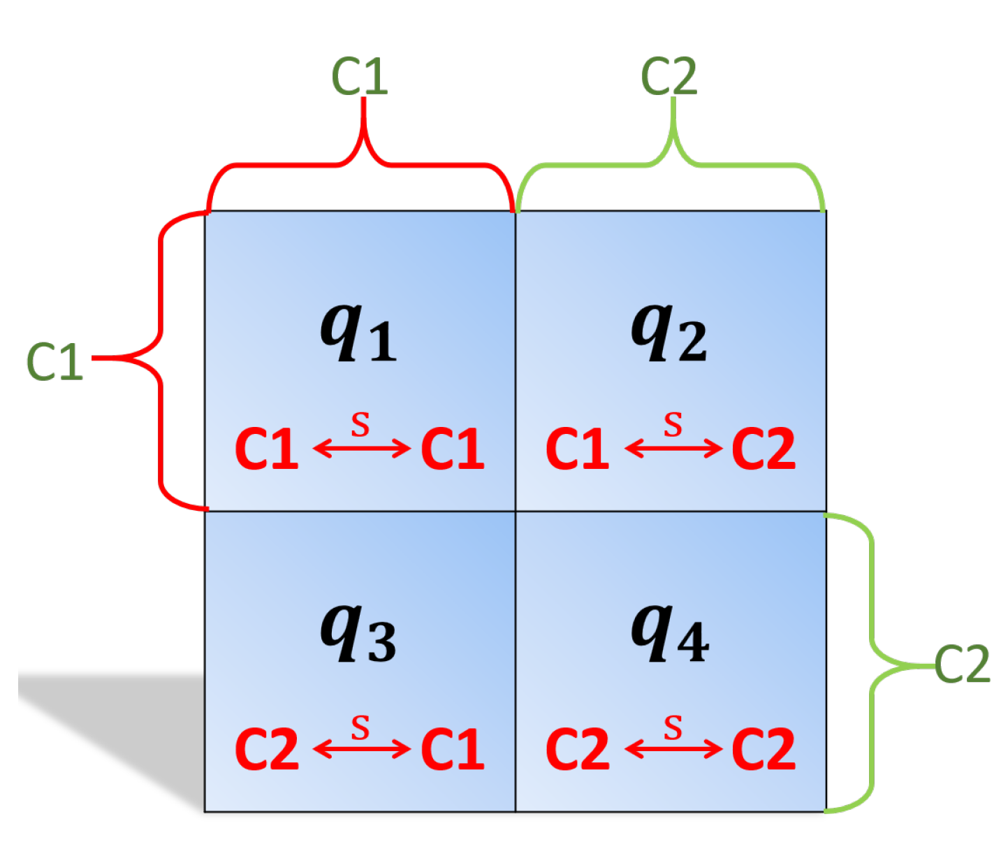
Whereas the above methods are based on optimization, the following discussion is based directly on the kernel matrices. Assume we have a binary classification problem; however, the following discussion and formulas extend to multi-class problems naturally. For a binary classification problem, assume we first reorder our training data such that class 1 data comes first, followed by class 2 data. This is a simplification for visualization sake; it is not a necessary step in our following indices. In this reordered kernel matrix there are four quadrants, $q_1$, $q_2$, $q_3$, and $q_4$ (shown in Figure 1) representing class 1 to class 1, class 1 to class 2, class 2 to class 1, and class 2 to class 2, respectively.

Intuitively, for a “good” kernel, $q_1$ and $q_4$ will each have high inner class proximities and $q_2$ (and, therefore, $q_3$ due to symmetry of the PSD kernel matrix) will have low between class proximities. The questions are: (1) how do we mathematically express these preferences, and (2) what truly are their implications, e.g., geometrically? In the following subsections we investigate different formula to answer these questions.

3.1. Key Factors for the Proposed Weight Assignments

In this article, our heuristic weight assignment is restricted to LCS (as is MKLGLp and GAMKLp). In future work we will consider the evaluation of combinations of kernels and their nonlinear aggregation. In order to determine the individual importance of each kernel, we first build a distribution for each quadrant, $f_{q1}$ to $f_{q4}$. The remainder of this article is based on the following simple but important properties.

Property 1. (Inner class similarity):

The mean of $f_{q1}$ and $f_{q4}$ should be high and $f_{q2}$ (and thus $f_{q3}$) should be low.

Property 2. (Class separation):

Distribution $f_{q3}$ should have as low of overlap as possible with distributions $f_{q1}$ and $f_{q4}$. There should be little-to-no confusion between objects in the two classes.

Property 3.  (Inner class spread):

Each quadrant should have low variation/spread.

There are many ways to measure Properties 1–3. The following subsections explore different mathematical formulations and why we might want to use them, and the experiments section demonstrates their performance on a collection of benchmark data.

First, we need to establish some notation. To measure the spread within each quadrant, the interquartile range (IQR) is computed, denoted herein as $IQR$, which is thought to be a more robust measure of distribution spread (except when the distribution is truly Normal Gaussian). This measure is robust to outliers as it measures the distance between the 25th and 75th percentile values of the given distribution. This results in a description of the distribution’s spread that is not as effected by outliers. Note, the pth percentile is a number such that approximately $p\%$ of the data, when sorted in ascending order, exist below the pth percentile and $(100-p)\%$ of the data exist above it.

3.2. Index 1 (Class Separation—Non-Normal Distribution): DiMKL${}_1$

The first index we propose focuses on class separation under a non-normal distribution of the kernel matrix promixities:

$$\mathrm{DiMKL}{}_1=exp\left(-\left(\frac{\sqrt{{({\mu }_{q_2}-IQ{R}_{q_2})}^2}}{2{\sigma }_{q_1}}\right)\right).$$

(5)

Specifically, DiMKL${}_1$ attempts to derive each kernel’s weight assignment based solely on the statistical information extracted from $q_1$ and $q_2$, the regions of the kernel matrix that exploits how proximate class 1 is to itself along with the interactions between classes 1 and 2. Equation (5) is rationalized as follows. To begin, it is feasible to explore the idea that we can adequately derive the kernel weights looking at only $q_1$ and $q_2$’s statistical information. That is, if a kernel matrix’s values for the cross-class proximity (i.e., $q_2$) is high for the quadrant as a whole, which is undesirable as it indicates that there is little-to-no class separability, taking the exponential of this large negative value would drive the weight assignment to 0. Conversely, if $q_2$ as a whole had highly dissimilar values, its statistical values would move towards 0 and taking the exponential of this tiny negative value would push the weight assignment to 1. In the numerator, the Euclidean distance between ${\mu }_{q_2}$ and $IQ{R}_{q_2}$ is computed, which, under such circumstances (i.e., specific to $q_2$) we desire ${\mu }_{q_2}\to 0$ and $IQ{R}_{q_2}\to 0$. Therefore, the closer these two values are to 0, the better we believe that the given kernel is at discriminating between the two classes. Similar desires are reflected in the denominator, but this is where statistical information pertaining to $q_1$ becomes involved. Specifically, ${\sigma }_{q_1}$ expresses the amount of spread that exists in $q_1$ (i.e., how ideal the intra-class proximities are to each other). Intuitively, $q_1$ is desired to possess some amount of spread, as this would indicate that the transformed feature space is generalizable, which will greatly help prevent overfitting.

3.3. Index 2 (Class Separation—Normal Distribution): DiMKL${}_2$

Our second index, again, looks for class separation, but assuming a Normal distribution of the kernel matrix proximities:

$$\mathrm{DiMKL}{}_2=exp\left(-\left(\frac{\sqrt{{({\mu }_{q_2}-{\sigma }_{q_2})}^2}}{2{\sigma }_{q_1}}\right)\right).$$

(6)

DiMKL${}_2$ takes a similar approach to that of DiMKL${}_1$ above. The key differentiation here is that $IQ{R}_{q_2}$ is replaced with the standard deviation in $q_2$, denoted as ${\sigma }_{q_2}$, in the numerator. This measure will be better fit for kernel matrices whose $q_2$ exhibits a Normal distribution, whereas DiMKL${}_1$ is better suited to handle non-Normal distributions.

3.4. Index 3 (Class Separation—Euclidean of Overlap): DiMKL${}_3$

For the third index, let $d_1$ and $d_2$ be defined as follows,

$$\begin{array}{cc}\hfill d_1& ={\mu }_{q_1}-IQ{R}_{q_1},\hfill \\ \hfill d_2& ={\mu }_{q_2}-IQ{R}_{q_2}.\hfill \end{array}$$

Then, we define DiMKL${}_3$ as

$$\mathrm{DiMKL}{}_3=\left(\sqrt{{(d_1-d_2)}^2}\right)\equiv |d_1-d_2|.$$

(7)

Through this measure, we are attempting to include more kernel matrix information when deriving the weights by including more statistical information from $q_1$. This measure has two terms, $d_1\mathrm{and}{d}_2$, that measure the distance between $q_1$ and $q_2$’s corresponding mean and IQR values, respectively. The Euclidean distance is computed between $d_1\mathrm{and}{d}_2$ with the goal being to obtain an idea of how much the two distributions overlap with one another. In the extreme (optimal) case, one quadrant’s distance, call it $d_a$, would approach 0, while the other quadrant’s distance, $d_b$, would approach 1 (i.e., no overlap, with extreme/optimal class separation). Therefore, under such a scenario, the calculated result would approach 1. Such a result leads to the given kernel receiving a very high weight assignment.

3.5. Index 4 (Class Separation—Euclidean of Means): DiMKL${}_4$

The fourth index is defined as:

$$\mathrm{DiMKL}{}_4=\frac{|{\mu }_{q_1}-{\mu }_{q_2}|}{\sqrt{(IQ{R}_{q_1}+IQ{R}_{q_2})}}.$$

(8)

This measure takes the absolute value, or Euclidean distance for the 1-D case, of the difference between ${\mu }_{q_1}$ and ${\mu }_{q_2}$ (in the numerator). For the denominator, we take the square root between the sum of $IQ{R}_{q_1}$ and $IQ{R}_{q_2}$. By taking the square root of the sum between $IQ{R}_{q_1}$ and $IQ{R}_{q_2}$, when the two IQR values are both very small, the square root has the effect of increasing the value and thus keeps the denominator from causing the result to blow up to a very large number that causes the given kernel to potentially demand full weight assignment.

3.6. Index 5 (Class Separation—Bhattacharyya): DiMKL${}_5$

Our fifth proposed heuristic considers the Bhattacharyya divergence measure on the kernel matrix proximities for deriving the weight assignments:

$$\mathrm{DiMKL}{}_5=\frac{b_1+b_2}{b_1+b_2+{\sigma }_{q_1}+{\sigma }_{q_2}+{\sigma }_{q_3}},$$

(9)

where

$$\begin{gathered} b_1=\frac{{({\mu }_{q_1}-{\mu }_{q_2})}^2}{4({\sigma }_{q_1}^2+{\sigma }_{q_2}^2)}+0.5ln\left(\frac{{\sigma }_{q_1}^2+{\sigma }_{q_2}^2}{2\sqrt{{\sigma }_{q_1}^2{\sigma }_{q_2}^2}}\right), \\ {b}_2=\frac{{({\mu }_{q_4}-{\mu }_{q_2})}^2}{4({\sigma }_{q_4}^2+{\sigma }_{q_2}^2)}+0.5ln\left(\frac{{\sigma }_{q_4}^2+{\sigma }_{q_2}^2}{2\sqrt{{\sigma }_{q_4}^2{\sigma }_{q_2}^2}}\right). \end{gathered}$$

This measure first takes the Bhattacharyya distance between $q_1$ and $q_2$ ($b_1$) as well as between $q_4$ and $q_2$ ($b_2$). Hence, the divergence between these distributions is being measured. This is effectively seeking to capture how similar the inner products are within each class as well as between classes.

4. Divergence Measures in the RKHS

In Section 3 we explored the measuring of divergence directly from the kernel matrices. This follows our intuition that classes should have high inner-class similarity and low between-class similarity. In this section we go further and explore the calculation of divergence instead explicitly on distributions in the RKHS. Thus, larger divergence values are directly related to a geometric interpretation of increasing separation between our class patterns in the underlying RKHS. The primary reason for exploring this route is to facilitate a comparison between a computationally expensive theoretical pathway, i.e., RKHS pathway, versus our inexpensive operations on the kernel matrices themselves.

Herein, without loss of generality, we focus on the Bhattacharyya distance in the RKHS—referred to as DiMKL${}_6$ hereafter. In [28], Zhou and Chellappa tackled this exact challenge mathematically with respect to ensemble similarity. Specifically, they formulated analytic expressions and algorithms to compute the Chernoff distance (of which the Bhattacharyya distance is a special case), Kullback–Leibler divergence, etc. In summary, it starts with formulating the mean and covariance (first and second-order statistics) in the RKHS. However, the covariance is rank-deficient. Thus, inverting it is impossible and an approximation is needed. The approximation of Zhou and Chellappa is based on three features: maintaining the principle structure of the covariance matrix, making sure that the solution is compact and regularized, and ensuring that it is easy to invert. Establishment of mathematical nomenclature and description of this procedure exceeds the space of the current article. The reader can refer to [28] for full detail.

5. Experiments

5.1. Feature Learning for Explosive Hazard Detection

We begin by investigating results on a real-world application for automatic detection of buried explosive hazards. This dataset was collected at a U.S. Army test site that contains multiple target and clutter types, burial depths, and times of day. Performance is summarized using normalized area under the curve (NAUC) values and experiments were performed using MATLAB. The test site was an arid environment and the targets varied in terms of metal content and burial depth. Herein, we denote the three lanes used for experimentation as Lane A, Lane B, and Lane C. Thermal variations were accounted for through the collection of data in both the morning and afternoon. We point out that Lane C was by far the most difficult due to a large number of weakly expressed targets. Lane-based three-fold cross-validation is used herein. Specifically, Fold-1 uses Lane A and B for training and tests on Lane C; Fold-2 uses Lane B and Lane C for training and tests on Lane A; and Fold-3 uses Lane A and Lane C for training and tests on Lane B.

Table 2. Data collection summary for each lane.

Lane	Number of Targets	Area (m${}^2$)	Metal Shallow	Metal Deep	Non-Metal Shallow	Non-Metal Deep
A	44	3626.9	21	3	11	9
B	50	4212.7	22	4	14	10
C	79	3944.8	31	15	21	12

summarizes this dataset.

Finally, we briefly discuss the features utilized, our improved Evolution COnstructed (iECO) features [15]. To over simplify, iECO is a feature learning technique that optimizes imagery data for feature extraction on a per image descriptor basis using a genetic algorithm (GA) as the basis for the search of optimal compositions of image transforms. At the end of the day, the GA produces a population of individuals who have learned unique approaches to extracting discriminative information for its assigned image descriptor. Herein, we employ three different image descriptors: Histogram of Oriented Gradients (HOG) [29,30,31], statistical descriptor (SD) [15], and edge histogram descriptor (EHD) [32,33]. For each, we investigate employing MKL to fuse the top five individuals learned for each image descriptor. Therefore, we have a total of 15 individuals—five for HOG, five for SD, and five for EHD. We also use a pre-screener score as a feature. There are numerous MKL-based approaches that one could use to attack this problem. For example, we could concatenate all of the iECO features into a single feature vector and use MK to fuse it with the pre-screener score. Another approach might be to group the features, i.e., concatenate all five iECO features for the HOG into a single feature vector, do the same for the SD and EHD iECO features, and then the pre-screener scores (thus, four groupings), and apply a single kernel to each grouping to fuse these feature space matrices via MKL.

Two experiments were conducted to investigate MKL and our proposed kernel weight assignment strategies. One is to employ a single RBF kernel to each iECO descriptor’s individual and the pre-screener score, giving 16 kernels to be fused. In [15], we showed that iECO individuals are extremely diverse, therefore each individual (even for the same image descriptor) finds very unique ways to extract discriminative information for its given image descriptor. Therefore, it is our conjecture that each individual has very useful ways of extracting information from the imagery and, thus, there is a strong desire to find a method to fuse these individual’s information together to strengthen the systems understanding of the imagery (e.g., classification accuracy). The second experiment is to apply a single RBF kernel to each group of features—concatenate all five HOG iECO individuals into a single feature vector, all five SD iECO individuals into a single feature vector, all five EHD iECO individuals into a single feature vector, and the pre-screener score. Therefore, we apply a total of four RBF kernels and investigate their performance.

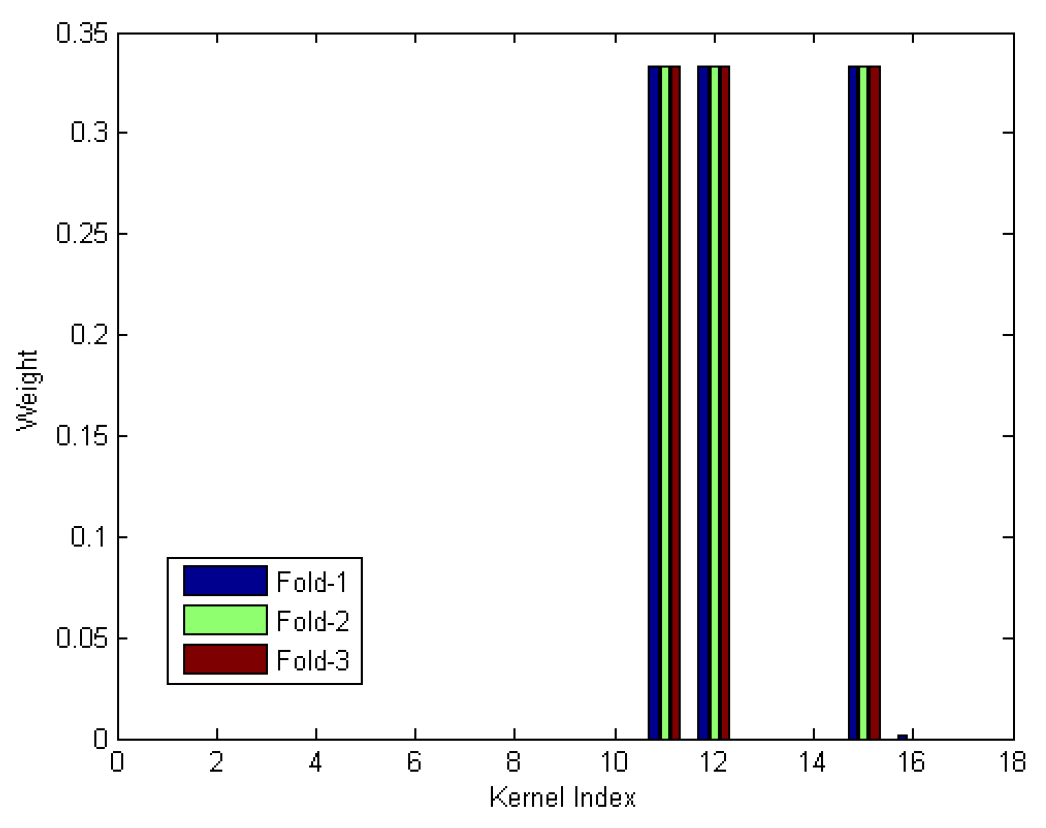
Results for our first experiment are summarized in

Table 3. Experiment 1: Fusing 16 RBF kernels. NAUC values are reported for each fold and MKL technique. Highest performing method is shown in blue; lowest performing is shown in red.

Learning Strategy	Weight Assignment	Fold-1	Fold-2	Fold-3
Fixed Rule	DiMKL${}_1$	0.290	0.560	0.570
Heuristic: Proposed Metrics	DiMKL${}_2$	0.336	0.643	0.570
	DiMKL${}_3$	0.335	0.633	0.611
	DiMKL${}_4$	0.333	0.633	0.598
	DiMKL${}_5$	0.335	0.616	0.617
	DiMKL${}_6$	0.336	0.633	0.565
Optimization Function	MKLGL	0.317	0.583	0.599

. Recall from above, this experiment applies a single RBF kernel to each iECO individual and to the pre-screener score, resulting in 16 kernels to be fused. We note that, herein, the RBF parameter ($\sigma$), for all 16 inputs was set to $\frac{1}{d_k}$, where $d_k$ is the dimensionality of input k. Additionally, we point out that results for DeFIMKL were not obtained due to there being 16 inputs, resulting in $2^{16}$ capacity terms, which is too much for our current solver and DeFIMKL implementation. Taking a closer look at Table 3, we see very encouraging results for our proposed heuristic measures, with four out of five performing either best overall or within a single percentage point of all other methods for each fold (the exception here is DiMKL${}_1$). Additionally, we see the need for multiple approaches to MKL weight assignment, as no single approach gives the overall best performance for each fold. However, because the proposed heuristic approaches are so simple in their computations, it is very efficient and fast (so one can easily run each metric and use the best performer for their given problem). For example, going forward, if we were considering using the training data from Fold-1 or Fold-2, we would want to implement DiMKL${}_2$’s weight assignment, and the kernel assignment utilizing DiMKL${}_5$ when using Fold-3 for training data. To understand why the performance for DiMKL${}_1$ is so poor, it is helpful to consider its derived weights, shown in Figure 2.

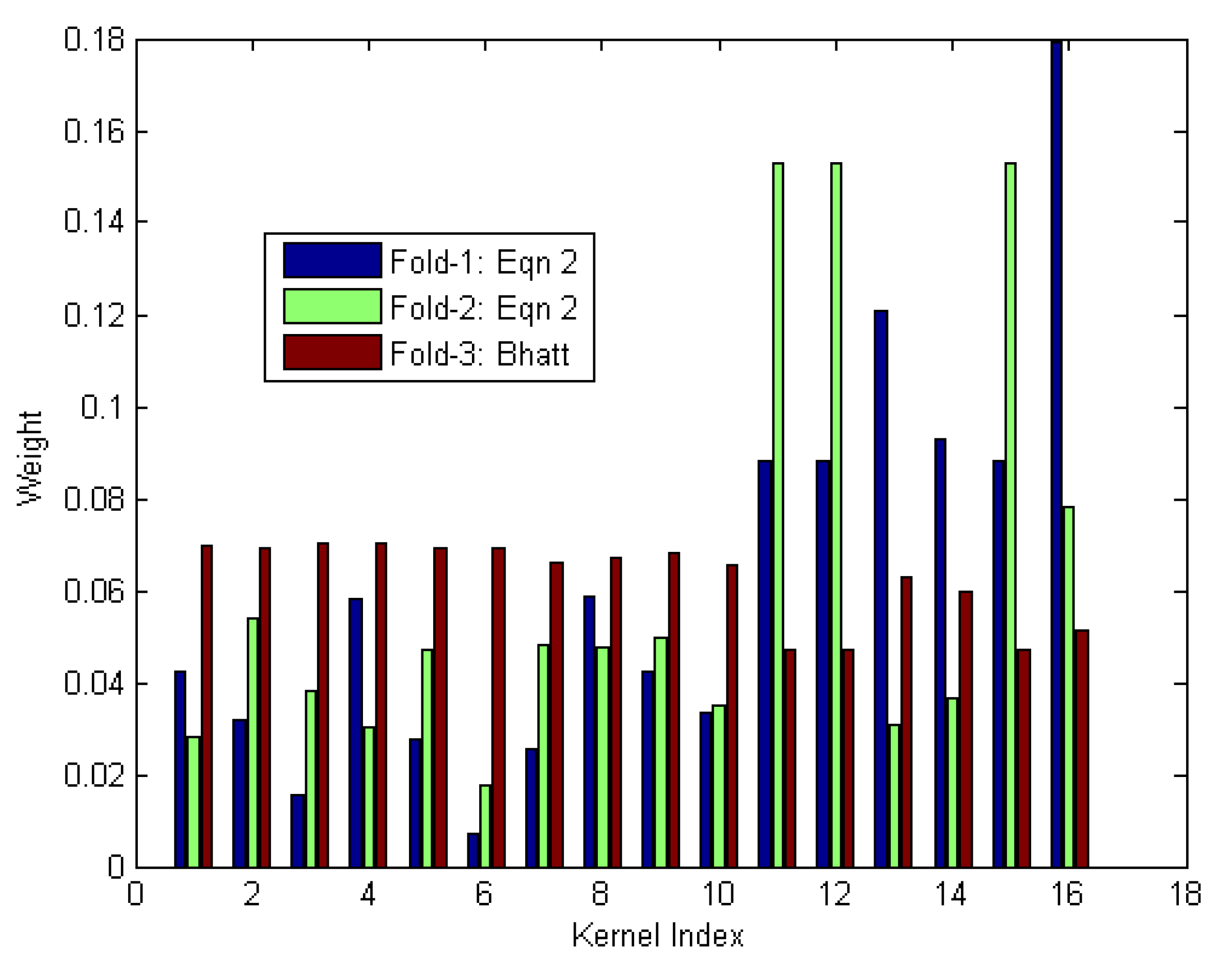
We quickly see that for this dataset and each of its folds, DiMKL${}_1$ attempted to focus the worth of the group on a relatively few individuals (in this case, only 3 of the 16 kernels were considered useful). However, as we alluded to earlier and have seen in our preliminary results, iECO individuals are very unique and bring their own useful information to the table, therefore the system as a whole is expected to perform better if it considers information from each pretty uniformly, with the exception of perhaps one or two instances having a little stronger weight assignment. This is reiterated when looking at the fixed rule approach, which simply provides a uniform weight assignment to each kernel. We see that this fixed rule strategy actually outperforms the very popular optimization approach, MKLGL, and is very close to most of our proposed metrics Finally, we show in Figure 3 the weights derived using DiMKL${}_2$ for Fold-1 and Fold-2, and using DiMKL${}_5$ for Fold-3. Therein, we see that, overall, weights are pretty uniformly distributed for this feature set (as expected).

Next, we present results for our second experiment in

Table 4. Experiment 2: Fusing four RBF kernels—one for each iECO descriptor grouping and the pre-screener score. MAUC values are reported for each fold and MKL technique. Highest performing method is shown in blue; lowest performing is shown in red.

Learning Strategy	Weight Assignment	Fold-1	Fold-2	Fold-3
Fixed Rule	Uniform	0.328	0.608	0.610
Heuristic: Proposed Metrics	DiMKL${}_1$	0.290	0.571	0.570
	DiMKL${}_2$	0.338	0.635	0.576
	DiMKL${}_3$	0.344	0.635	0.608
	DiMKL${}_4$	0.334	0.628	0.596
	DiMKL${}_5$	0.330	0.611	0.610
	DiMKL${}_6$	0.334	0.633	0.571
Optimization Function	MKLGL	0.318	0.595	0.578
	DeFIMKL	0.317	0.607	0.614

, which applied a single RBF kernel to each grouping of features, for a total of four kernels to be fused. Here, we see the robustness and generalizability our metrics possess as a similar story is expressed as in the previous experiment. Specifically, all but one of our proposed metrics performs either best, or extremely close to being the best. The one instance in which DeFIMKL outperformed our heuristic metrics, we actually have two methods that are within a single percentage point of DeFIMKL. Again, DiMKL${}_1$’s performance suffers on this dataset, performing worst in all Folds. It is also important to discuss the results of MKLGL here, which is a commonly used optimization approach to MKL. Here, we see that it consistently under performs our proposed metrics, especially on Fold-2 and Fold-3. This is very likely contributed to its susceptibility to over-fitting the training data and not generalizing well. These methods should theoretically find an optimal solution; however, given that real-world data rarely (if ever) captures the entire data distribution space, empirical evidence indicates these methods suffer under such conditions.

5.2. Benchmark Datasets

Three benchmark UCI datasets [34] are used to evaluate the proposed metrics. Specifically, we use the Sonar, Ionosphere, and Breast Cancer Wisconsin datasets. These are summarized in

Table 5. UCI Benchmark Datasets.

Dataset	Instances	Features	Classes
Sonar	208	60	2
Ionosphere	351	34	2
Breast Cancer Wisconsin	683	10	2

. The data were split into training and testing data, with 80% being randomly assigned to the training data and the remaining for testing. Furthermore, each experiment was executed 100 times for statistical analysis and algorithm sensitivity. For all experiments, 5 RBF kernels were implemented with the following $\sigma$ parameters: $\sigma =\{2\times {10}^{-3},\frac{1}{d},\frac{5}{d},\frac{10}{d},\frac{25}{d}\}$, where d is the number of features.

Classification results/accuracies and their standard deviations for the 100 trials on the UCI benchmark datasets (80% training, 20% testing) for our proposed metrics, MKLGL, DeFIMKL, and GAMKLp are shown in

Table 6. Classification accuracy and standard deviation for 100 trials on UCI benchmark datasets. Note: 80% training, 20% testing. Highest performing method is shown in blue; lowest performing is shown in red.

Learning Strategy	Method	Sonar	Ionosphere	Breast Cancer
SKSVM	Individual K${}_1$	58.39 (11.22)	71.14 (6.01)	96.16 (1.55)
	Individual K${}_2$	78.17 (6.36)	92.14 (3.01)	97.08 (1.29)
	Individual K${}_3$	84.63 (5.98)	94.31 (2.46)	96.66 (1.43)
	Individual K${}_4$	84.56 (5.83)	94.27 (2.36)	96.29 (1.44)
	Individual K${}_5$	82.15 (7.97)	92.34 (2.74)	95.64 (1.53)
Heuristic: Proposed Metrics	DiMKL${}_1$	86.17 (5.54)	94.07 (2.36)	96.57 (1.46)
	DiMKL${}_2$	81.68 (6.35)	94.71 (2.39)	97.13 (1.26)
	DiMKL${}_3$	85.22 (5.77)	94.70 (2.32)	97.10 (1.27)
	DiMKL${}_4$	85.17 (5.93)	94.69 (2.33)	97.09 (1.29)
	DiMKL${}_5$	83.41 (6.53)	94.57 (2.34)	97.05 (1.26)
	DiMKL${}_6$	84.75 (6.10)	94.63 (2.41)	97.09 (1.28)
Optimization Strategies	DeFIMKL	82.60 (7.89)	93.01 (2.96)	96.11 (1.63)
	GAMKL	85.60 (5.22)	94.49 (2.49)	97.06 (1.48)
	MKLGL	83.31 (7.98)	94.08 (2.32)	95.68 (1.49)

. Immediately, DiMKL${}_1$ proves its utility for such a task, whereas if we looked solely at the explosive hazards detection experiments, we might wonder why even use DiMKL${}_1$. On all three datasets, DiMKL${}_1$ produces very competitive results, in terms of classification accuracy and standard deviations (relative to each dataset). For the Sonar dataset, we do see a pretty high value for standard deviation, but this is the result of the individual kernels themselves expressing much variation depending on the partitioning of the data. Since our heuristic approach is based on the kernel matrix itself, such variation in the heuristic fusion methods can be expected. For all experiments spanning these benchmark datasets, the proposed heuristics outperform the optimization function strategies, at times by a relatively large margin. This is achieved with the additional major benefit of efficiency and a low computational cost, as these do not require multiple iterations nor optimizers to be implemented.

Next, we take a deeper look at the weights being learned by each method. For the weight assignments reported in

Table 7. Sonar: highest performing method is shown in blue; lowest performing is shown in red.

Sonar	DiMKL${}_1$	DiMKL${}_2$	DiMKL${}_3$	DiMKL${}_4$	DiMKL${}_5$	DiMKL${}_6$	GAMKL	MKLGL	Ind Kernel Perf
${\kappa }_{1,wt}$	$0.00$	$0.00$	$0.00$	$0.09$	$0.22$	$0.08$	$0.13$	$0.00$	$58.54\%$
${\kappa }_{2,wt}$	$0.00$	$0.81$	$0.07$	$0.14$	$0.15$	$0.23$	$0.22$	$0.00$	$87.80\%$
${\kappa }_{3,wt}$	$0.45$	$0.05$	$0.07$	$0.25$	$0.18$	$0.25$	$0.21$	$1.00$	$90.24\%$
${\kappa }_{4,wt}$	$0.23$	$0.08$	$0.12$	$0.25$	$0.20$	$0.34$	$0.22$	$0.00$	$91.68\%$
${\kappa }_{5,wt}$	$0.31$	$0.04$	$0.72$	$0.25$	$0.22$	$0.34$	$0.22$	$0.00$	$82.93\%$
Fused Performance	92.68%	$87.80\%$	$90.24\%$	$90.24\%$	$90.24\%$	$90.24\%$	87.19%	$90.24\%$

,

Table 8. Ionosphere: highest performing method is shown in blue; lowest performing is shown in red.

Ionosphere	DiMKL${}_1$	DiMKL${}_2$	DiMKL${}_3$	DiMKL${}_4$	DiMKL${}_5$	DiMKL${}_6$	GAMKL	MKLGL	Ind Kernel Perf
${\kappa }_{1,wt}$	$0.00$	$0.00$	$0.00$	$0.09$	$0.26$	$0.07$	$0.12$	$0.00$	$52.86\%$
${\kappa }_{2,wt}$	$0.01$	$0.15$	$0.17$	$0.19$	$0.16$	$0.25$	$0.20$	$0.00$	$88.57\%$
${\kappa }_{3,wt}$	$0.32$	$0.40$	$0.22$	$0.24$	$0.17$	$0.25$	$0.23$	$0.99$	$94.29\%$
${\kappa }_{4,wt}$	$0.32$	$0.37$	$0.23$	$0.24$	$0.19$	$0.24$	$0.23$	$0.00$	$95.71\%$
${\kappa }_{5,wt}$	$0.34$	$0.08$	$0.38$	$0.24$	$0.23$	$0.20$	$0.22$	$0.00$	$92.86\%$
Fused Performance	$95.71\%$	$95.71\%$	$95.71\%$	$95.71\%$	$95.71\%$	$95.71\%$	96.42%	94.28%	N/A

and

Table 9. Breast Cancer: highest performing method is shown in blue; lowest performing is shown in red.

Breast Cancer	DiMKL${}_1$	DiMKL${}_2$	DiMKL${}_3$	DiMKL${}_4$	DiMKL${}_5$	DiMKL${}_6$	GAMKL	MKLGLL	Ind Kernel Perf
${\kappa }_{1,wt}$	$0.00$	$0.00$	$0.00$	$0.09$	$0.21$	$0.06$	$0.14$	$0.00$	$68.38\%$
${\kappa }_{2,wt}$	$0.01$	$0.79$	$0.40$	$0.21$	$0.19$	$0.24$	$0.12$	$0.00$	$97.79\%$
${\kappa }_{3,wt}$	$0.33$	$0.00$	$0.26$	$0.23$	$0.19$	$0.24$	$0.25$	$0.99$	$96.32\%$
${\kappa }_{4,wt}$	$0.33$	$0.12$	$0.19$	$0.23$	$0.20$	$0.23$	$0.25$	$0.00$	$96.32\%$
${\kappa }_{5,wt}$	$0.33$	$0.09$	$0.14$	$0.23$	$0.20$	$0.23$	$0.24$	$0.00$	$94.12\%$
Fused Performance	96.32%	98.53%	$97.79\%$	$97.06\%$	$97.79\%$	$97.06\%$	$96.69\%$	96.32%	N/A

, a single randomly selected trial from the 100 trials is reported. The purpose is to provide analysis on the metrics in a real setting on benchmark datasets. We do omit inclusion of DeFIMKL weights in these tables for compactness, though we note their performance was comparable but did not differentiate itself as a best performer. Note, naming is as follows: ${\kappa }_{i,wt}$ denotes the ith kernel’s weight assignment, with the row of values being the weight assigned for the given kernel. Additionally, the classification accuracy for each individual kernel is provided in the last column of the table. In each table, the highest performer for the given trial is highlighted in green and the lowest performer is highlighted in red.

First and foremost, we see that each proposed equation, DiMKL${}_1$–DiMKL${}_6$, derives its weight assignments uniquely, with none of the measures assigning weights in a similar manner. This has the obvious benefit that none of the equations are redundant in their exploitation of information and therefore can each provide distinct ways of characterizing the kernel matrices. This can allow for a quick understanding of the behavior of different kernels implemented such as how a particular dataset’s features are being separated (e.g., is the intra-class information for class 1 providing the discriminative information or do we have features that separate the classes, seen through cross-class separation but does not discriminate within classes very well).

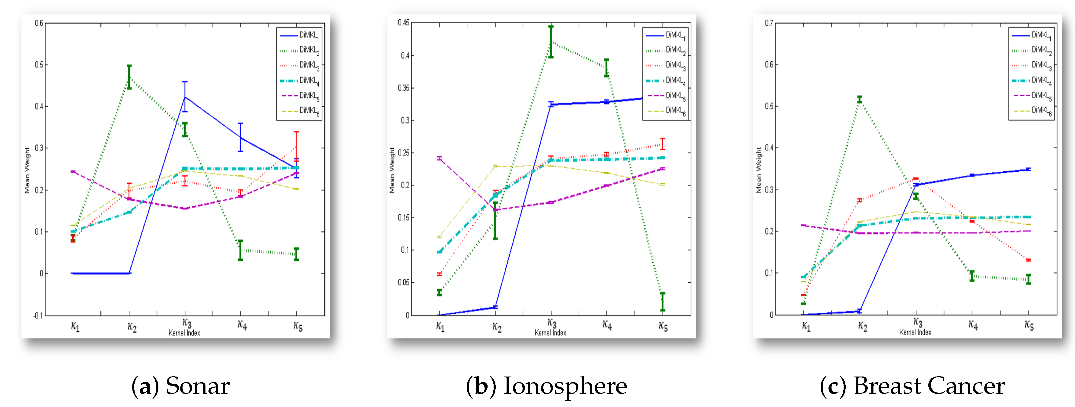
Second, the two measures based on the Bhattacharyya distance, DiMKL${}_5$ and DiMKL${}_6$, appear to distribute the weights close to uniformity for all three experiments reported in Table 7, Table 8 and Table 9. It is important to note that DiMKL${}_6$ does a better job at identifying the very poor kernels, as it assigned a near zero-valued weight assignment in all three cases to the worst kernel (i.e., ${\kappa }_1$, which had the worst individual performance on all three benchmark datasets). Beyond this, there are signs that each equation, if given the same $\sigma$ parameter RBF kernel, tends to assign its weights in a similar manner, regardless of the dataset. This is not universal nor is it constant between all datasets. This is a mere observation when looking at the weight assignments for Table 7, Table 8 and Table 9 that there does appear to be some trend in the weights assigned, but there does not appear to be any type of linear correlation present. Evidence also supports this when analyzing the standard deviation of the weight assignments for each metric across all 100 trials, shown in Figure 4. In Figure 4a–c, the standard deviation is shown by intervals, and it is easily seen that there is very little spread for each kernels weight assignment.

5.3. Computational Complexity

Finally, we consider the proposed indices’ computational complexity. Let n be an array of values representing those in $q_1$ and m be an array of values representing those in $q_2$. The computational complexity of the indices computed directly on the kernel matrix is $O(n\times m)$. If we assume the worst case scenario, the size of $n=m$, then we have $O\left(n^2\right)$. We provide the computational time for DiMKL${}_1$–DiMKL${}_6$ and MKLGL on synthetic data of increasing size in

Table 10. Computational complexity: empirical study (reported in seconds); n represents the size of the array.

Method	n = 500	n = 1000	n = 5000	n = 10,000	n = 25,000
DiMKL${}_1$	$0.0002$	$0.0003$	$0.0005$	$0.0008$	$0.0023$
DiMKL${}_2$	$0.0006$	$0.0005$	$0.0010$	$0.0011$	$0.0019$
DiMKL${}_3$	$0.0008$	$0.0006$	$0.0009$	$0.0011$	$0.0018$
DiMKL${}_4$	$0.0006$	$0.0004$	$0.0004$	$0.0005$	$0.0009$
DiMKL${}_5$	$0.0001$	$0.0001$	$0.0001$	$0.0003$	$0.0006$
DiMKL${}_6$	$0.0949$	$0.4117$	$0.8293$	$1.2882$	$3.7554$
MKLGL	$0.3637$	$0.3760$	$10.1476$	$45.3782$	$305.3951$

. For perspective, considering $n=10,000$, DiMKL${}_1$ is over $56\mathrm{k}\times$ faster than the corresponding MKLGL approach.

6. Conclusions

Herein, novel MKL weight assignment metrics are proposed to address the complexities and shortcomings of optimization strategies used for deriving MK weights. To address these issues, DiMKL${}_1$–DiMKL${}_6$ provide a computationally efficient and highly effective heuristic approach for weight assignment based solely on the statistical information within a kernel’s similarity matrix. These metrics allow for the automatic determination of kernel weights without the need for highly complex and sophisticated learning strategies that are susceptible to overfitting the training data and/or getting stuck in local minima due to poor initialization. While there is not a single metric given to encompass this task, the proposed derivations are simple to implement and very efficient (i.e., low computational complexity). Further, it is similar to one of the needs for MKL: for different problems/applications, different kernels will be better suited to exploiting discriminative information and the combination of MK can help exploit additional information that is not easily captured by a single kernel. Hence, there is a need for different kernel assignment heuristics as each looks at the kernel’s discriminative information differently when assigning weights. While the proposed indices do not provide any convergence guarantees, their experimental results on several UCI benchmark datasets and an automatic explosive hazards detection dataset validate the utility of our proposed metrics and why there is a need for multiple metrics.

References

- Cortes, C.; Vapnik, V. Support-vector networks. Mach. Learn. 1995, 20, 273–297. [Google Scholar] [CrossRef]
- Chang, C.C.; Lin, C.J. LIBSVM: A library for support vector machines. ACM Trans. Intell. Syst. Technol. 2011, 2, 27:1–27:27. Available online: http://www.csie.ntu.edu.tw/~cjlin/libsvm (accessed on 20 March 2018). [CrossRef]
- Das, S.; Abraham, A.; Konar, A. Automatic kernel clustering with a multi-elitist particle swarm optimization algorithm. Pattern Recognit. Lett. 2008, 29, 688–699. [Google Scholar] [CrossRef]
- Kim, D.W.; Lee, K.Y.; Lee, D.; Lee, K.H. Evaluation of the performance of clustering algorithms in kernel-induced feature space. Pattern Recognit. 2005, 38, 607–611. [Google Scholar] [CrossRef]
- Liao, L.; Lin, T.; Li, B. MRI brain image segmentation and bias field correction based on fast spatially constrained kernel clustering approach. Pattern Recognit. Lett. 2008, 29, 1580–1588. [Google Scholar] [CrossRef]
- Mika, S.; Schölkopf, B.; Smola, A.J.; Müller, K.R.; Scholz, M.; Rätsch, G. Kernel PCA and de-noising in feature spaces. In Proceedings of the Advances in Neural Information Processing Systems, Denver, CO, USA, 29 November–4 December 1999; pp. 536–542. [Google Scholar]
- Schölkopf, B.; Smola, A.; Müller, K.R. Kernel principal component analysis. In Proceedings of the International Conference on Artificial Neural Networks, Lausanne, Switzerland, 8–10 October 1997; Springer: Berlin/Heidelberg, Germany, 1997; pp. 583–588. [Google Scholar]
- Kim, K.I.; Franz, M.O.; Scholkopf, B. Iterative kernel principal component analysis for image modeling. IEEE Trans. Pattern Anal. Mach. Intell. 2005, 27, 1351–1366. [Google Scholar]
- Price, S.R.; Anderson, D.T.; Havens, T.C. Fusion of iECO image descriptors for buried explosive hazard detection in forward-looking infrared imagery. Proc. SPIE 2015, 9454, 945405. [Google Scholar]
- Price, S.R.; Murray, B.; Hu, L.; Anderson, D.T.; Havens, T.C.; Luke, R.H.; Keller, J.M. Multiple kernel based feature and decision level fusion of iECO individuals for explosive hazard detection in FLIR imagery. In Detection and Sensing of Mines, Explosive Objects, and Obscured Targets XXI; SPIE Defense+ Security; International Society for Optics and Photonics: Bellingham, WA, USA, 2016; p. 98231G. [Google Scholar]
- Pinar, A.J.; Rice, J.; Hu, L.; Anderson, D.T.; Havens, T.C. Efficient Multiple Kernel Classification Using Feature and Decision Level Fusion. IEEE Trans. Fuzzy Syst. 2017, 25, 1403–1416. [Google Scholar] [CrossRef]
- Schölkopf, B.; Smola, A.J. Learning with Kernels: Support Vector Machines, Regularization, Optimization, and Beyond; MIT Press: Cambridge, MA, USA, 2002. [Google Scholar]
- Schölkopf, B.; Smola, A.J.; Williamson, R.C.; Bartlett, P.L. New support vector algorithms. Neural Comput. 2000, 12, 1207–1245. [Google Scholar] [CrossRef] [PubMed]
- Hsu, C.W.; Chang, C.C.; Lin, C.J. A practical guide to support vector classification. 2003. Available online: https://www.csie.ntu.edu.tw/~cjlin/papers/guide/guide.pdf (accessed on 20 March 2018).
- Price, S.R.; Anderson, D.T.; Luke, R.H. An improved evolution-constructed (iECO) features framework. In Proceedings of the 2014 IEEE Symposium on Computational Intelligence for Multimedia, Signal and Vision Processing (CIMSIVP), Orlando, FL, USA, 9–12 December 2014; pp. 1–8. [Google Scholar] [CrossRef]
- Lu, K.; Zhao, J.; Zhang, J.; Qin, C. Multiple Kernel Learning via Ensemble Artifice in Reproducing Kernel Hilbert Space. In Proceedings of the 2020 International Conference on Cyber-Enabled Distributed Computing and Knowledge Discovery (CyberC), Chongqing, China, 29–30 October 2020; IEEE: Piscataway, NJ, USA, 2020; pp. 264–267. [Google Scholar]
- Varma, M.; Babu, B.R. More generality in efficient multiple kernel learning. In Proceedings of the 26th Annual International Conference on Machine Learning, Montreal, QC, Canada, 14–18 June 2009; pp. 1065–1072. [Google Scholar]
- Suzuki, T.; Tomioka, R. SpicyMKL: A fast algorithm for multiple kernel learning with thousands of kernels. Mach. Learn. 2011, 85, 77–108. [Google Scholar] [CrossRef]
- Han, Y.; Yang, Y.; Li, X.; Liu, Q.; Ma, Y. Matrix-Regularized Multiple Kernel Learning via (r,p) Norms. IEEE Trans. Neural Netw. Learn. Syst. 2018, 29, 4997–5007. [Google Scholar] [CrossRef] [PubMed]
- Xu, L.; Luo, B.; Tang, Y.; Ma, X. An efficient multiple kernel learning in reproducing kernel Hilbert spaces (RKHS). Int. J. Wavelets Multiresolution Inf. Process. 2015, 13, 1550008. [Google Scholar] [CrossRef]
- Banerjee, S.; Das, S. Kernel selection using multiple kernel learning and domain adaptation in reproducing kernel hilbert space, for face recognition under surveillance scenario. arXiv 2016, arXiv:1610.00660. [Google Scholar]
- Gönen, M.; Alpaydın, E. Multiple kernel learning algorithms. J. Mach. Learn. Res. 2011, 12, 2211–2268. [Google Scholar]
- Xu, Z.; Jin, R.; Yang, H.; King, I.; Lyu, M.R. Simple and Efficient Multiple Kernel Learning by Group Lasso; Fürnkranz, J., Joachims, T., Eds.; ICML; Omnipress: Madison, WI, USA, 2010; pp. 1175–1182. [Google Scholar]
- Pinar, A.; Havens, T.C.; Anderson, D.T.; Hu, L. Feature and decision level fusion using multiple kernel learning and fuzzy integrals. In Proceedings of the 2015 IEEE International Conference on Fuzzy Systems (FUZZ-IEEE), Istanbul, Turkey, 2–5 August 2015; IEEE: Piscataway, NJ, USA, 2015; pp. 1–7. [Google Scholar]
- de Diego, I.; Moguerza, J.; Munoz, A. Combining kernel information for support vector classification. In Proceedings of the International Workshop on Multiple Classifier Systems, Cagliari, Italy, 9–11 June 2004; pp. 102–111. [Google Scholar]
- de Diego, I.M.; Muñoz, A.; Moguerza, J.M. Methods for the combination of kernel matrices within a support vector framework. Mach. Learn. 2010, 78, 137. [Google Scholar] [CrossRef]
- Moguerza, J.M.; Munoz, A.; de Diego, I.M. Improving Support Vector Classification via the Combination of Multiple Sources of Information; SSPR/SPR; Springer: Berlin/Heidelberg, Germany, 2004; pp. 592–600. [Google Scholar]
- Zhou, S.K.; Chellappa, R. From sample similarity to ensemble similarity: Probabilistic distance measures in reproducing kernel hilbert space. IEEE Trans. Pattern Anal. Mach. Intell. 2006, 28, 917–929. [Google Scholar] [CrossRef] [PubMed]
- Edelman, S.; Intrator, N.; Poggio, T. Complex Cells and Object Recognition. 1997. Available online: https://shimon-edelman.github.io/Archive/nips97.pdf (accessed on 3 June 2016).
- Lowe, D.G. Object recognition from local scale-invariant features. In Proceedings of the Seventh IEEE International Conference on Computer Vision, Kerkyra, Greece, 20–27 September 1999; Volume 2, pp. 1150–1157. [Google Scholar]
- Dalal, N.; Triggs, B. Histograms of oriented gradients for human detection. In Proceedings of the International Conference on Computer Vision and Pattern Recognition, CVPR 2005, San Diego, CA, USA, 20–26 June 2005; IEEE Computer Society: Washington, DC, USA, 2005; Volume 1, pp. 886–893. [Google Scholar]
- Frigui, H.; Gader, P. Detection and discrimination of land mines in ground-penetrating radar based on edge histogram descriptors and a possibilistic k-nearest neighbor classifier. IEEE Trans. Fuzzy Syst. 2009, 17, 185–199. [Google Scholar] [CrossRef]
- Stone, K.; Keller, J.; Anderson, D.; Barclay, D. An automatic detection system for buried explosive hazards in FL-LWIR and FL-GPR data. SPIE Def. Secur. Sens. 2012, 8357, 83571E. [Google Scholar]
- Lichman, M. UCI Machine Learning Repository. 2013. Available online: https://archive.ics.uci.edu/ml/index.php (accessed on 14 October 2017).
Figure 1.
Four quadrants for a supervised two class kernel matrix. The similarity represented in each quadrant is denoted with respect to class. C1: class 1, C2: class 2, and : similarity between.
Figure 2.
Bar plot showing the weights derived by DiMKL for each Fold.
Figure 3.
Bar plot showing the highest performing weight assignments for each Fold. Specifically, for Fold-1 and Fold-2, DiMKL was the best performer, and for Fold-3, DiMKL. Finally, we see evidence validating that each iECO individual brings unique and useful information as the weight assignments are nearly uniform.
Figure 4.
Mean weights and standard deviations (error bars) for each individual kernel for the six proposed heuristic MKL weight assignment equations.