A Clustering Ensemble Framework with Integration of Data Characteristics and Structure Information: A Graph Neural Networks Approach

Abstract

Clustering ensemble is a research hotspot of data mining that aggregates several base clustering results to generate a single output clustering with improved robustness and stability. However, the validity of the ensemble result is usually affected by unreliability in the generation and integration of base clusterings. In order to address this issue, we develop a clustering ensemble framework viewed from graph neural networks that generates an ensemble result by integrating data characteristics and structure information. In this framework, we extract structure information from base clustering results of the data set by using a coupling affinity measure After that, we combine structure information with data characteristics by using a graph neural network (GNN) to learn their joint embeddings in latent space. Then, we employ a Gaussian mixture model (GMM) to predict the final cluster assignment in the latent space. Finally, we construct the GNN and GMM as a unified optimization model to integrate the objectives of graph embedding and consensus clustering. Our framework can not only elegantly combine information in feature space and structure space, but can also achieve suitable representations for final cluster partitioning. Thus, it can produce an outstanding result. Experimental results on six synthetic benchmark data sets and six real world data sets show that the proposed framework yields a better performance compared to 12 reference algorithms that are developed based on either clustering ensemble architecture or a deep clustering strategy.

1. Introduction

Data clustering, also known as cluster analysis, is the process of partitioning a set of data objects into some clusters based on a similarity measure without any prior knowledge. The objects in each cluster are similar to each other, and different from data objects in other clusters [1]. All of these clusters are usually referred to as a clustering result. The core of data clustering is to discover the inherent structure from the unlabeled data. Thus, it is usually employed as an effective tool to understand raw data in the initial phase of processing, particularly for the problems where prior knowledge is absent or expensive to obtain. Driven by the demand of acquiring knowledge from various complicated data, clustering analysis has become a research hotspot. Over the past decades, many studies have focused on the solution of data clustering from diverse perspectives, such as clustering algorithms with different similarity criteria [2], extensions and modification for particular data types [3], identifying the optimal number of clusters [4], subspace clustering and multiview clustering [5,6], clustering results evaluation [7], and applications of data clustering [8].

Unlike supervised learning methods, data clustering is essentially an ill-posed problem [9] because the results of different clustering algorithms can be equally accepted without prior knowledge. In other words, any clustering result may be superior to others in a particular pattern distribution. This problem results in a dilemma: users need to select an appropriate clustering algorithm according to the inherent characteristics of data and domain knowledge. The clustering ensemble appears in this background, and it can generate an excellent and stable cluster assignment by combining multiple clustering results [10]. Clustering ensemble outperforms the single clustering algorithm in several aspects [11,12]: (i) the average performance of clustering ensemble on different data types and pattern distributions is superior to its optimal ensemble member; (ii) it can obtain a consistent result that cannot be achieved by any single clustering algorithm; (iii) it is more robust to noises, outliers, and sampling changes than single clustering algorithm; (iv) it outperforms the single clustering algorithm in terms of parallelizability and scalability; and (v) it can integrate multiple clustering results generated from distributed data sources or features. Generally, clustering ensemble comprises two main phases. In the first phase, a group of base clustering results is produced. In the second phase, a consensus function is designed to generate a final cluster assignment by combing base clustering results. The base clustering members can be produced in many ways, such as by using different clustering algorithms, employing one clustering algorithm with different parameters, and utilizing subsets of data or features [13]. The typical methods used to design a consensus function include a relabeling strategy [14], feature-based methods [15,16], pairwise-similarity-based algorithms [17,18], and graph-based approaches [19,20]. In general, three ensemble-information matrices [11] can be acquired from the base clustering results: the label-assignment matrix, pairwise similarity matrix, and binary cluster association matrix. Each ensemble strategy mentioned above utilizes one of these matrices to combine base clustering results. That is to say, the clustering ensemble results of these methods are derived either from a reorganized data description in feature space or from the relationships between data objects in structure space. In reality, the data characteristics that are expressed by features or attributes and the structure information manifested as relationships between objects are two presentations of the data from different perspectives. Therefore, both of them provide valuable guidance on producing the final ensemble result. However, the existing clustering ensemble algorithms, according to our knowledge, seldom consider combining these two data descriptions in the design of the consensus function.

Data characteristics and structure information focus on different aspects of data description. Thus, their combination can potentially improve thereliability of clustering ensemble. With this motivation, we develop a novel clustering ensemble framework to integrate data characteristics with structure information. To serve this purpose, our work is focused on addressing the following two key issues: (i) What structural information should be employed to construct the consensus function? Many local relationships are commonly used to describe structure information, such as the label-assignment information originally obtained from an ensemble, co-association matrix, or associations between data objects or those among clusters [13]. In general, the structural information represents the implicit relationships between data objects. It includes not only the local similarity between objects, but also a global structure implying the intrinsic pattern of the data. Therefore, using only the local structure to design the clustering consensus function is far from sufficient, and determining how to effectively extract and utilize suitable structure information is an important problem. (ii) How can we integrate data characteristics and structure information to produce the consensus clustering result? If only concentrating on data characteristics, the deep clustering algorithms [21,22,23] provide an effective data partitioning strategy using the powerful representation learning ability of deep learning. For example, an autoencoder (AE) [24] is a commonly used framework with multiple layers, in which, each layer captures specific latent information from data characteristics, while in a clustering ensemble context, one can acquire various forms of structure information from the data and its base clusterings. Therefore, what is the interaction relationship between data characteristics and structure information in the generation of the final clustering result? Furthermore, how can these two different types of information be combined elegantly, and how can they be represented in a suitable form for clustering ensemble? These problems constitute the other key issue of our work.

To address the first problem, we intend to capture the structural information of the data from a set of base clusterings. All of the base clusterings are produced on the same data; thus, some forms of relationships certainly exist between base clusterings, between clusters, and between objects. Viewed from this aspect, the intrinsic structure information can be captured from a set of base clustering results by explicating and coupling the above relationships.

We employ a variational graph autoencoder (VGAE) module [25] to cope with the second key issue by learning the joint representations of data characteristics and structure information suitable for the clustering objective. On this basis, we derive a joint optimization model that incorporates representation learning and consensus cluster partitioning into a unified framework.

In this study, we propose a novel framework, namely clustering ensemble viewed from graph embedding (CEvGE), to integrate data characteristics with structure information by employing the powerful representation ability of GNNs. Our work can be viewed as an improvement on a clustering ensemble model by learning appropriate representations in the latent space. In addition, it can be viewed as an improvement on a deep clustering method by imposing a global structure constraint. Our main contributions can be summarized as follows:

(i)

We develop a novel clustering ensemble framework viewed from GNNs that produces the ensemble result by exploiting both data characteristics and structure information.

(ii)

We reconstruct raw data as an object similarity graph, and integrate data characteristics and structure information elegantly by learning their joint representations in a variational GNN. We employ a Gaussian mixture model (GMM) to predict the consensus cluster assignment for the latent embeddings, which is a natural model for clustering.

(iii)

We construct a unified optimization model to integrate the objectives of joint embedding learning and final cluster assignment, in which, clustering can provide a correct guidance for embedding learning.

(iv)

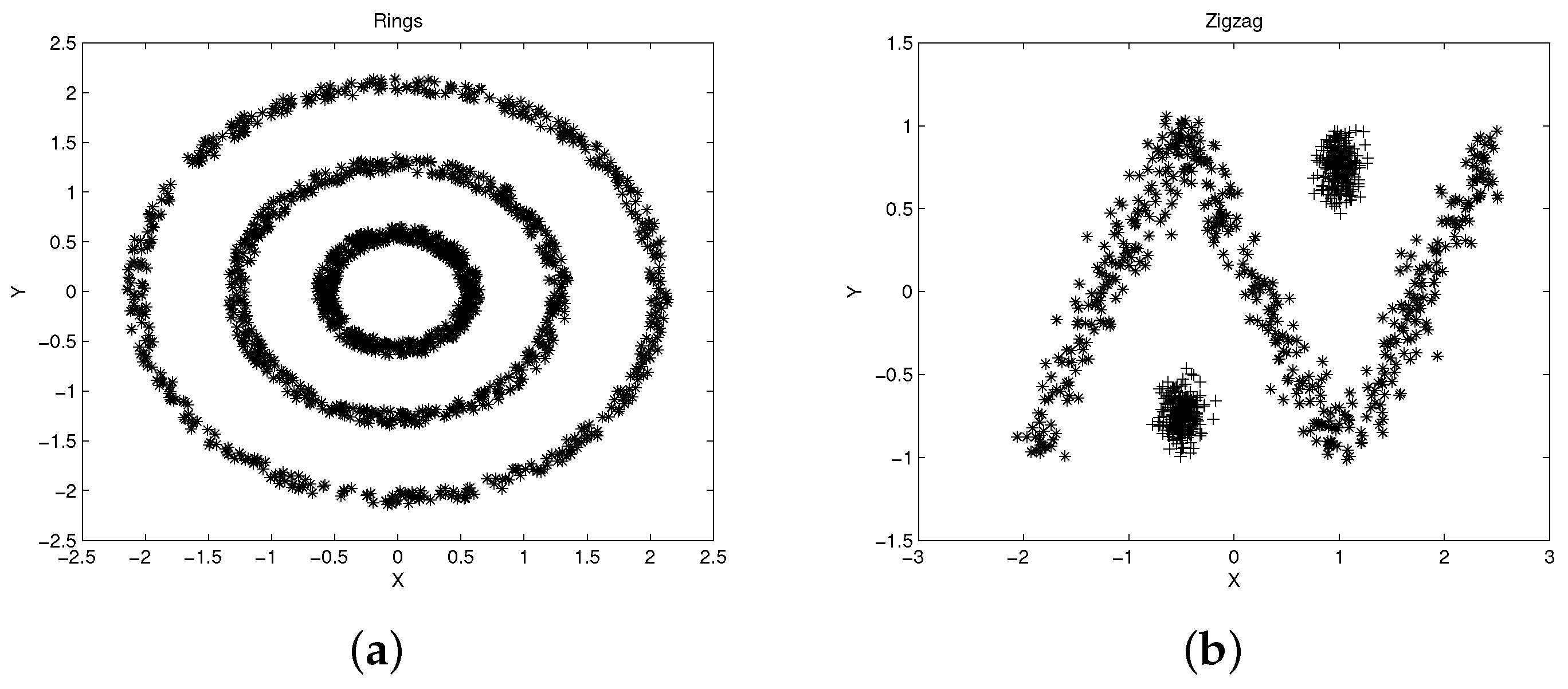
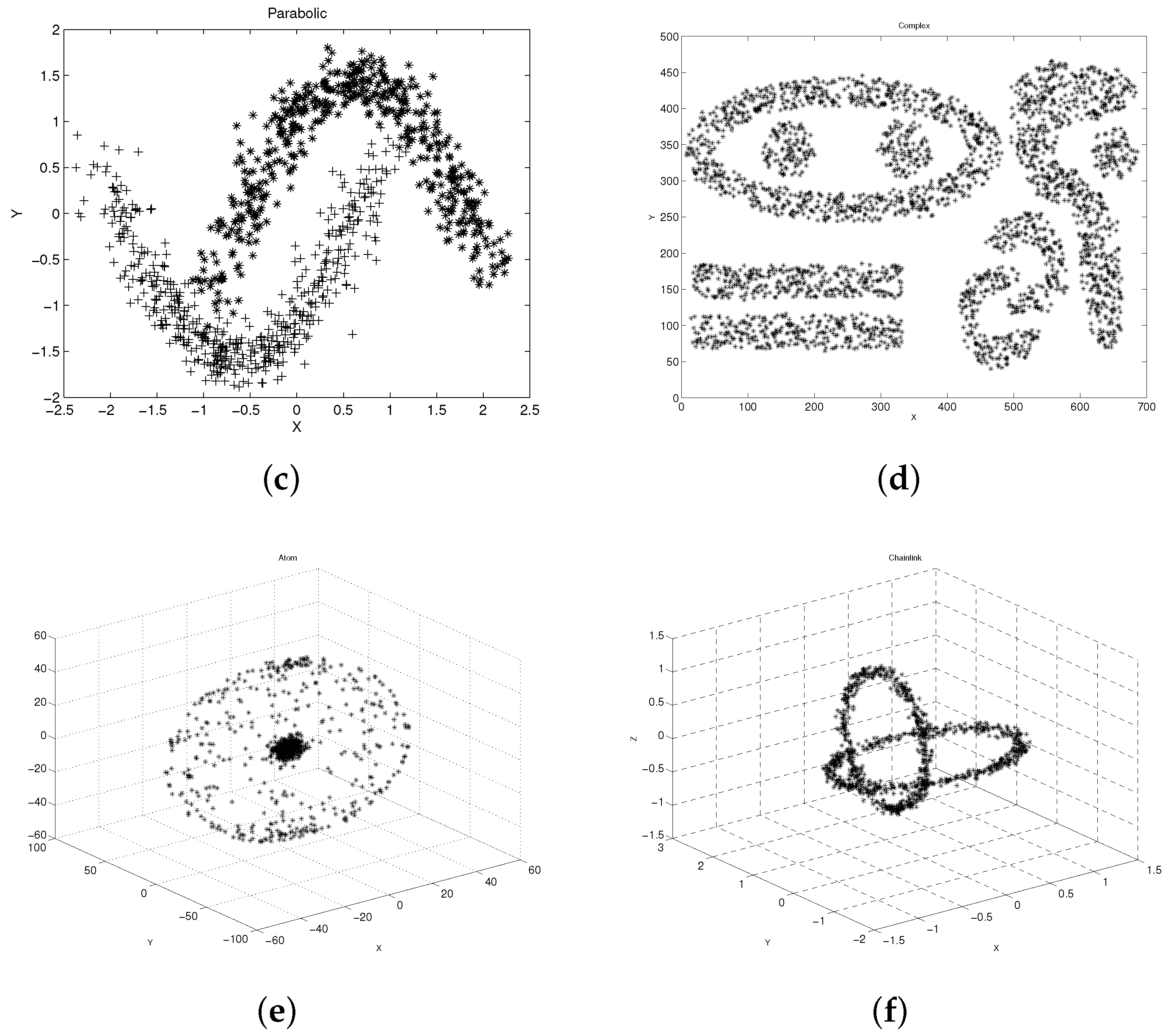
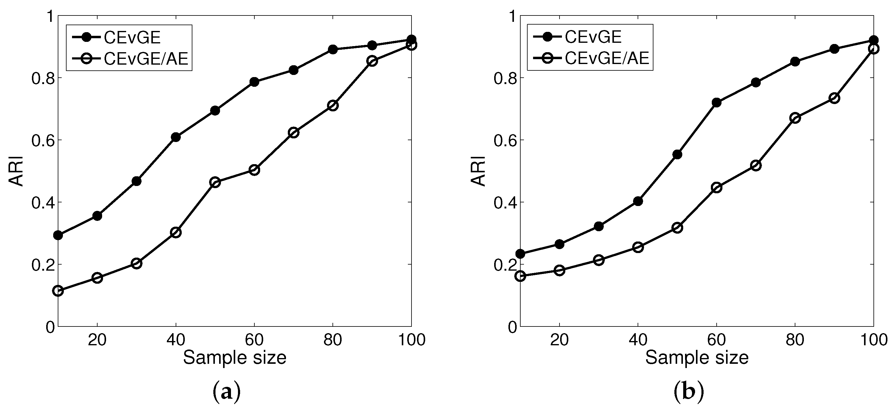
We conduct extensive experiments on synthetic and real-world data sets. The results demonstrate the validity and superiority of our framework against reference algorithms.

The remainder of this paper is organized as follows. Section 2 introduces some closely related works. In Section 3, we discuss the construction and implementation of our CEvGE framework in detail. In Section 4, we compare the CEvGE with several state-of-the-art clustering ensemble models and deep clustering algorithms in a series of experiments Finally, we conclude this work in Section 5.

2. Related Work

In this section, we introduce works related to the AE and variational autoencoder (VAE), deep clustering, and graph embedding.

2.1. AE and VAE

The AE can be regarded as a nonlinear generalization of PCA used to reduce data dimensionality, in the form of a multilayer neural network with a small middle layer [24]. It consists of three basic elements: an adaptive, multilayer encoder network that transforms the high-dimensional data into low-dimensional codes; a decoder network with a similar structure that recovers data from the codes; and a loss function that measures the lost information caused by dimensionality reduction. Driven by the popularity of various deep learning models, especially the generative adversarial networks (GANs), the AE has been regarded as at the forefront of generative modeling. Various extended AE models have been developed successively. In general, these extended models fall into three categories [26]: (i) instantiation-based models trained by combining them with other learning schemes, such as the convolutional autoencoder (CAE) and extreme learning machine autoencoder (ELMAE), etc.; (ii) regularization-based models implemented by introducing regularization constraints into the loss function, including the sparse autoencoder, contractive autoencoder, and information theoretic-learning autoencoder, etc.; and (iii) variational inference-based models, such as the VAE and adversarial autoencoder (AAE).

Using a similar encoder–decoder structure, the VAE is in fact deeply rooted in the variational Bayesian methods [27], which map input data into a distribution in latent space rather than a fixed vector In the VAE, the decoder network can be viewed as a generative module that generate new samples similar to but not identical to input data. The necessary assumptions for the VAE are relatively weak, and it can be trained fast by backpropagation. Furthermore, the error introduced by approximation in the VAE is arguably small. These merits make the VAE a very popular generative model. To improve the performance of the VAE for data with a complex distribution, some works attempt to enhance the prior assumption for latent variables by introducing a Bayesian probabilistic mixture model. For example, Jiang et al. [28] approximated the prior distribution of latent variables by a mixture of Gaussians, and develped an improved VAE model, namely variational deep embedding (VaDE). Nalisnick et al. [29] also enhanced the prior description in the VAE using a GMM, and proposed a deep latent Gaussian mixture model (DLGMM) that employs multiple inference networks to generate variational posterior distribution. Another similar work is the DGG developed by Yang et al. [30], which constructs a single generative model with an isotropic Gaussian mixture prior description.

2.2. Deep Clustering with the Encoder–Decoder Schema

Recently, driven by the powerful representation ability of the deep neural network (DNN), some works attempted to improve the clustering performance by introducing the DNN to learn effective data representations for the clustering objective. Tian et al. constructed a two-stage deep clustering framework that utilized a DNN to acquire feature representations in subspace, and then divided clusters using these learned features. To guide the DNN to learn suitable representations for cluster assignment, some later works tried to incorporate a clustering objective into the deep learning framework. For example, Xie et al. employed an incomplete AE to learn data embeddings, and designed an assistant distribution to estimate cluster assignment for the learned embeddings. In that model, called deep embedded clustering (DEC), the cluster assignment and model training are achieved simultaneously in a self-learning schema. Guo et al. [31] introduced a complete autoencoder to improve DEC by overcoming the misguiding problem in embedding learning. In this way, the clustering loss can provide a positive guidance for embedding learning on maintaining the original distribution pattern. Similarly, another deep learning model proposed by Guo et al., namely deep convolutional embedded clustering (DCEC), utilized a convolutional AE and a single-layer classifier to learn the data representations and the cluster distributions, respectively. In this model, the DNN is trained by minimizing the reconstruction loss and the estimation error measured by relative entropy. In [32], the authors elected some representative data objects as landmarks and measured the similarity of landmarks between all data objects as the input of the autoencoder. They combined embedding learning and cluster assignment to further enhance the clustering performance. They also employed clustering loss to update the cluster centers and parameters of AE simultaneously. Bo et al. [33]. proposed a structural deep clustering network (SDCN) model to integrate the structural information into deep clustering, in which a delivery operator was designed to transfer the representations learned by autoencoder to the corresponding GCN layer. On this basis, they also developed a dual self-supervised mechanism to unify the two different deep neural architectures and guide the update of the whole model. Wang et al. [34] designed a dual-stacked autoencoder feature embedded clustering (DSAFEC) for human activity recognition (HAR) that uses dual-stacked autoencoder features (DSAF) to learn new representations for the original input and then predicts cluster assignment probabilities for the learned representations by employing a softmax regression.

In the above deep clustering algorithms, embeddings are learned effectively by the AE with a strict one-to-one correlation to input data. However, the pattern of learned embedding depends on the training data; as a result, the distribution in latent space is discontinuous. That is to say, the clustering performance would degrade due to the decoded data possibly losing some characteristics implied in the original data. To address this issue, some later works apply VAE as the embedding learning network for deep clustering, rather than AE. In VAE, the latent variables sampled from the learned distributions can effectively capture the statistics of original data. In addition, the decoder can generate data objects that help the clustering process acquire more information about the inherent distribution of original data. For example, Jiang et al. [28] developed an unsupervised generative deep clustering model called VaDE, in which, the latent embeddings are learned by a DNN and the cluster distributions are predicted by a GMM. In the optimization of VaDE, the SGVB estimator and the reparameterization trick are introduced. For the clustering problem of high-dimensional data, Li et al. [35] proposed a VAE-based model named the latent tree variational autoencoder (LTVAE)that produces several clustering results for high-dimensional data using distinct portions of features. They described latent embeddings in a tree structure, and used the location of each cluster in the tree to organize the data relationships. Hwang et al. [36] addressed the issue of the clustering complex and high-dimensional wafer maps in semiconductor manufacturing by proposing a variational deep clustering algorithm, namely one-step VAE+DPGMM. In this algorithm, a GMM is implemented into a VAE framework to extract more suitable features for the clustering environment, and a Dirichlet process is further applied in the variational autoencoder mixture framework for automated one-step clustering. Compared with conventional two-step clustering methods, the model can considerably increase the chance to distinguish small differences in wafer map patterns.

All of the deep clustering algorithms mentioned above introduce the powerful representational ability of DNNs for clustering tasks based on an AE or VAE framework. However, they all focus on improving the conventional clustering approaches rather than the clustering ensemble context. Additionally, they only explore data relationships in feature space and neglect the information in structure space, which is also an important description of the data pattern. In a clustering ensemble context, the overlooked structure information is just hidden in the set of base clustering results. This fact motivates us to introduce the powerful representation learning ability of DNNs to clustering ensemble, and to exploit data characteristics and structure information together to produce the consensus clustering result.

2.3. Graph Embedding

As a ubiquitous form of data organization, a graph provides a natural tool to express structure information of data, as it can record relationships between data objects effectively. To incorporate the non-Euclidean graph data into machine learning models, graph embedding is always used to encode the graph from high-dimensional, sparse space into a low-dimensional, compact, and continuous feature space, where characteristics in the original graph are preserved as much as possible. Various graph embedding models can be abstracted to an encoder–decoder framework, in which, the encoder maps each vertex to a low-dimensional embedding and the decoder reconstructs the graph from the learned embeddings [37]. In general, the objective of the encoder–decoder graph embedding model is optimized by minimizing a certain reconstruction loss. Graph embedding models can be divided into two categories: (i) shallow embedding models, which are largely inspired by classic matrix factorization techniques [38] or random walks [39], and always utilize an “embedding lookup” encoder function; and (ii) generalized encoder–decoder architectures, which construct highly complex encoders often using GNNs to map topology and vertex attributes together into a low-dimensional latent space [40,41]. In the latter category, some works aggregate local topology to learn graph embedding in a VAE framework. For example, the model in [25] constructs a VAE-based learning framework, where a graph convolutional network (GCN) and an inner product function are employed as the encoder and the decoder, respectively. To overcome the inferior embedding problem in real-world graph data, Pan et al. [42] proposed an adversarially regularized VGAE, in which, the embedding learned by the encoder is forced to match a prior distribution by using an adversarial training scheme. To solve the data corruption issue, Kang et al. [43] proposed a graph learning scheme to learn reliable graphs from the real-world noisy data by adaptively removing noise and errors in the raw data. The model can also be viewed as a robust version of manifold regularized robust principle component analysis (RPCA), where the quality of the graph plays a critical role.

3. The Proposed Framework

For a set of N data objects $\mathbf{X}={\left\{{\mathbf{x}}_i\right\}}_{i=1}^N$ in the D-dimensional space, let $\mathsf{\Pi }={\left\{{\pi }_t\right\}}_{t=1}^T$ represent a set of T base clusterings for $\mathbf{X}$, where ${\pi }_t={\left\{C_{\gamma }^t\right\}}_{\gamma =1}^{k_t}$ is the $t^{}$th clustering member, $k_t$ denotes the number of clusters in ${\pi }_t$, and $C_{\gamma }^t$ is the ${\gamma }^{}$th cluster. For the object ${\mathbf{x}}_i$, ${\lambda }_i^t$ denotes its cluster label in the $t^{}$th base clustering. The label set, including all of the different labels in ${\pi }_t$, is denoted by ${\mathsf{\Lambda }}_t$, and the objects assigned with label ${\lambda }_i^t$ in ${\pi }_t$ are marked as $s_t\left({\lambda }_i^t\right)$. The task of clustering ensemble is to produce a consensus partition ${\pi }^{*}={\left\{C_k^{*}\right\}}_{k=1}^K$ for $\mathbf{X}$ by combining all of the base clusterings, where K is the number of clusters in ${\pi }^{*}$, and $C_k^{*}$ denotes the $k^{}$th cluster in the consensus result.

3.1. Overview of the Framework

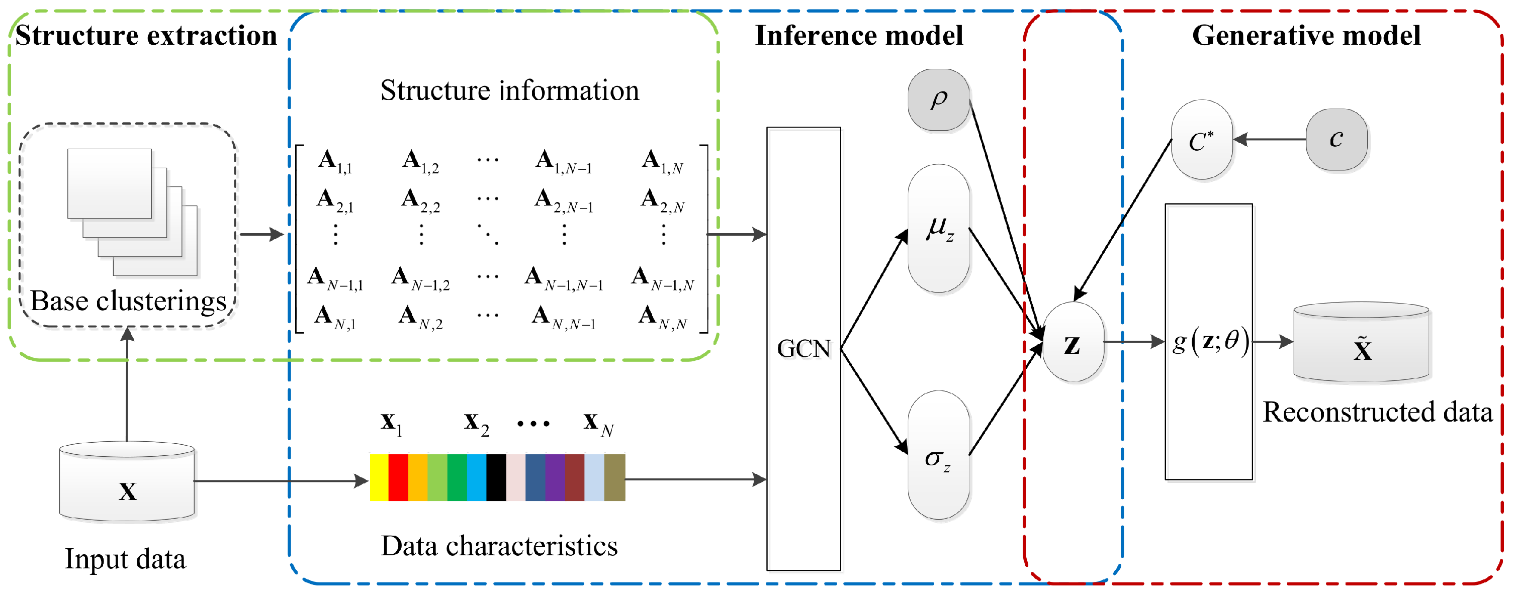
The integral construction of the CEvGE framework is illustrated in Figure 1. In the CEvGE, the structure information of data is firstly extracted from a set of base clusterings. With the help of the structure information, the data set can be reorganized as an an object similarity graph. Then, the data characteristics and structure information are integrated in a VGAE module viewed from graph embedding perspective. In the latent space, a GMM is applied to predict the consensus cluster assignment for the joint embedding. Finally, the VGAE module and the GMM are trained jointly in a unified optimization model, which integrates objectives of graph embedding and consensus cluster assignment.

3.2. Extraction of Structure Information

An affinity matrix is always constructed to describe the data structure, where each element represents relationships between two data objects evaluated by a certain similarity measure. Thus, an adequate similarity measure that can express the inherent data relationships comprehensively is very important when describing structure information. In the original data space before clustering, the data structure can be directly captured by calculating pairwise similarity. However, this form of structure information can only describe presentational relationships from a local perspective. In the clustering ensemble context, we can explore extra structure information from a set of base clusterings. On the one hand, data relationships are reflected in the inner-dependence within a base clustering, and, on the other hand, they are also implied in the inter-dependence among different base clusterings. As a result, the global structure information that reveals an intrinsic pattern of data can be acquired by uncovering the coupling relationships between base clusterings, between clusters, and between data objects. In this work, the coupling relationships are in terms of two elements: interactions between base clusterings and between data objects [17]. We propose capturing and incorporating them to tease out the implicit global relationships in the data, which will be used subsequently to construct the affinity matrix.

3.2.1. Coupling of Base Clusterings

All base clustering results are different partitionings on the same data; as a result, there must be some relationships among these base results. From intra and inner perspectives, the coupling of base clusterings comprises two components: the intra-coupling impresses the interaction between cluster labels within one base clustering, whereas the inner-coupling indicates the interaction between two base clusterings. According to this idea, we use the coupled clustering similarity for clusters (CCSC) between two cluster labels to describe the coupling relationship of base clusterings:

$$Si{m}_t^{\pi }\left({\lambda }_i^t,{\lambda }_j^t|{\left\{{\mathsf{\Lambda }}_o\right\}}_{o=1}^T\right)=Si{m}_t^{\pi -Ia}\left({\lambda }_i^t,{\lambda }_j^t\right)Si{m}_t^{\pi -Ie}\left({\lambda }_i^t,{\lambda }_j^t|{\left\{{\mathsf{\Lambda }}_o\right\}}_{o\ne t}\right),$$

(1)

where $Si{m}_t^{\pi }\left({\lambda }_i^t,{\lambda }_j^t|{\left\{{\mathsf{\Lambda }}_o\right\}}_{o=1}^T\right)$ is the CCSC between two cluster labels ${\lambda }_i^t$ and ${\lambda }_j^t$. $Si{m}_t^{\pi -Ia}$$\left({\lambda }_i^t,{\lambda }_j^t\right)$ is the intra-coupled clustering similarity (IaCS) between ${\lambda }_i^t$ and ${\lambda }_j^t$, used to describe the intra-coupling of base clusterings by calculating the frequency of cluster labels within a base clustering. $Si{m}_t^{\pi -Ie}\left({\lambda }_i^t,{\lambda }_j^t|{\left\{{\mathsf{\Lambda }}_o\right\}}_{o\ne t}\right)$ is the inter-coupled relative similarity (IeRS) between ${\lambda }_i^t$ and ${\lambda }_j^t$ based on another base clustering ${\pi }_o$, used to characterize the intra-coupling of base clusterings by comparing the co-occurrence of the cluster labels among different base clusterings, where ${\mathsf{\Lambda }}_o$ is the label set of ${\pi }_o$. The IaCS is defined as:

$$Si{m}_t^{\pi -Ia}\left({\lambda }_i^t,{\lambda }_j^t\right)=\frac{\left|s_t\left({\lambda }_i^t\right)\right|\left|s_t\left({\lambda }_j^t\right)\right|}{\left|s_t\left({\lambda }_i^t\right)\right|+\left|s_t\left({\lambda }_j^t\right)\right|+\left|s_t\left({\lambda }_i^t\right)\right|\left|s_t\left({\lambda }_j^t\right)\right|}.$$

(2)

The IeRS is defined as:

$$Si{m}_t^{\pi -Ie}\left({\lambda }_i^t,{\lambda }_j^t|{\left\{{\mathsf{\Lambda }}_o\right\}}_{o\ne t}\right)={\displaystyle \sum }_{o=1,o\ne t}^T{\omega }_{o}Si{m}_{t|o}\left({\lambda }_i^t,{\lambda }_j^t|{\mathsf{\Lambda }}_o\right),$$

(3)

where ${\omega }_o\in \left[0,1\right]$ is the weight of the base clustering ${\pi }_o$, ${\displaystyle {\displaystyle \sum }_{o=1,o\ne t}^T}{\omega }_o=1$, and $Si{m}_{t|o}\left({\lambda }_i^t,{\lambda }_j^t|{\mathsf{\Lambda }}_o\right)$ is defined as:

$$Si{m}_{t|o}\left({\lambda }_i^t,{\lambda }_j^t|{\mathsf{\Lambda }}_o\right)=\sum _{{\lambda }^o\in \mathsf{\Omega }}min\left\{\frac{\left|s_o\left({\lambda }^o\right)\cap s_t\left({\lambda }_i^t\right)\right|}{\left|s_t\left({\lambda }_i^t\right)\right|},\frac{\left|s_o\left({\lambda }^o\right)\cap s_t\left({\lambda }_j^t\right)\right|}{\left|s_t\left({\lambda }_j^t\right)\right|}\right\}.$$

(4)

In Equation (4), $\mathsf{\Omega }$ denotes the set $L_o\left(s_t\left({\lambda }_i^t\right)\right)\cap L_o\left(s_t\left({\lambda }_j^t\right)\right)$, where $L_o\left(s_t\left({\lambda }_i^t\right)\right)$ is the label set of $s_t\left({\lambda }_i^t\right)$ in ${\pi }_o$.

3.2.2. Coupling of Data Objects

Similarly, the coupling relationships between objects can also be described from the following two perspectives. In terms of the intra-perspective, we use the intra-coupled object similarity (IaOS) to measure the similarity between two objects, which is defined as the average sum of the CCSC between the associated cluster labels ranging over all of the base clusterings. The IaOS between ${\mathbf{x}}_i$ and ${\mathbf{x}}_j$ can be calculated as

$$Si{m}^{IaOS}\left({\mathbf{x}}_i,{\mathbf{x}}_j\right)=\frac{1}{T}\sum _{t=1}^{T}Si{m}_t^{\pi }\left({\lambda }_i^t,{\lambda }_j^t|{\left\{{\mathsf{\Lambda }}_o\right\}}_{o=1}^T\right).$$

(5)

whereas, from the inter-perspective, we reflect the interaction between data objects by mining their neighbors’ correlation. Accordingly, we utilize the common neighbors between two objects to mesure the inter-coupled object similarity (IeOS), which is defined as

$$Si{m}^{IeOS}\left({\mathbf{x}}_i,{\mathbf{x}}_j\right)=\frac{1}{N}\left|\left\{{\mathbf{x}}_n\in \mathbf{X}|{\mathbf{x}}_n\in N_{{\mathbf{x}}_i}\cap N_{{\mathbf{x}}_j}\right\}\right|.$$

(6)

In Equation (6) where $Si{m}^{IeOS}\left({\mathbf{x}}_i,{\mathbf{x}}_j\right)$ denotes the IeOS between objects ${\mathbf{x}}_i$ and ${\mathbf{x}}_j$. $N_{{\mathbf{x}}_i}$ represents the neighbor set of ${\mathbf{x}}_i$, and is defined as

$$N_{{\mathbf{x}}_i}=\left\{{\mathbf{x}}_n|\kappa \left({\mathbf{x}}_i,{\mathbf{x}}_n\right)\ge \theta \right\}.$$

(7)

$\kappa (·,·)$ is a Gaussian kernel function with a threshold $\theta \in [0,1]$, which is defined as

$$\kappa \left({\mathbf{x}}_i,{\mathbf{x}}_n\right)=\frac{1}{{\alpha }_i}exp\left(-\frac{\phi {({\mathbf{x}}_i,{\mathbf{x}}_n)}^2}{2{\vartheta }^2}\right),$$

(8)

where ${\alpha }_i>0$ and $\vartheta >0$ are the normalizer and width of the kernel function, respectively, and $\phi (·)$ denotes a certain similarity measure for data objects.

The location of a data object in a clustering is determined by the cluster it belongs to. Accordingly, we can integrate the relationships from the inner-perspectives and inter-perspectives together through the associated clusters. In particular, we induce the coupled similarity of objects by specifying the similarity measure employed in Equation (8) to be IaOS, and we have

$$\kappa {\left({\mathbf{x}}_i,{\mathbf{x}}_n\right)}^{IaOS}=\frac{1}{{\alpha }_i}exp\left(-\frac{Si{m}^{IaOS}{({\mathbf{x}}_i,{\mathbf{x}}_n)}^2}{2{\vartheta }^2}\right).$$

(9)

Then, the IeOS can be converted to a new similarity measure for objects, namely coupled clustering and object similarity (CCOS). The CCOS between ${\mathbf{x}}_i$ and ${\mathbf{x}}_j$ can be calculated as

$$Si{m}^{CCOS}\left({\mathbf{x}}_i,{\mathbf{x}}_j\right)=\frac{1}{N}\left|\left\{{\mathbf{x}}_n\in \mathbf{X}|{\mathbf{x}}_n\in N_{{\mathbf{x}}_i}^{IaOS}\cap N_{{\mathbf{x}}_j}^{IaOS}\right\}\right|,$$

(10)

where the neighbor sets are defined as $N_{{\mathbf{x}}_i}^{IaOS}=\left\{{\mathbf{x}}_n|{\kappa }^{IaOS}\left({\mathbf{x}}_i,{\mathbf{x}}_n\right)\ge \theta \right\}$ and $N_{{\mathbf{x}}_j}^{IaOS}=\left\{{\mathbf{x}}_n\right|{\kappa }^{IaOS}$$\left({\mathbf{x}}_j,{\mathbf{x}}_n\right)\ge \theta \}$, respectively. In this manner, both the intra-coupled and inter-coupled relationships between data objects are considered in the CCOS. In the meantime, the intra-coupled and inter-coupled interactions between base clusterings are also taken into account by the new similarity measure.

3.2.3. Structure Information Organized by a Affinity Matrix

According to the above discussion, a global structure description can be extracted from a set of base clusterings, i.e., CCOS. Compared with previous local similarity measurements, the CCOS expresses comprehensive relationships between data objects from multiple perspectives by exploiting base clusterings. Thus, we use the CCOS to construct an affinity matrix ${\mathbf{A}}_{N\times N}$ that organizes the structure information of the data. The element $A_{i,j}$ in the matrix is denoted as

$$A_{i,j}=Si{m}^{CCOS}\left({\mathbf{x}}_i,{\mathbf{x}}_j\right).$$

(11)

3.3. Clustering Ensemble Viewed from Graph Embedding Perspective

The affinity matrix of structure information can be seen as geometric constraints of the data. As a result, we can reorganize the input data $\mathbf{X}$ as an objects similarity graph $G(\mathbf{X},\mathbf{A})$, which includes both the characteristics and structure of the data. In this way, the clustering ensemble task on $\mathbf{X}$ is transformed into a clustering problem on the reorganized graph $G(\mathbf{X},\mathbf{A})$. To this end, we develop a joint model within the VGAE framework. In this model, data characteristics and structure information are integrated by learning their joint embeddings in latent space, and, subsequently, a GMM is utilized to predict the final cluster assignments for the latent embeddings.

3.3.1. Inference Model

The inference model is used to integrate data characteristics and structure information jointly by mapping the graph-reorganized data to latent embeddings, which are parameterized by a two-layer GCN as

$$q\left(\mathbf{Z}|\mathbf{X},\mathbf{A}\right)=\sum _{i=1}^{N}q\left({\mathbf{z}}_i|\mathbf{X},\mathbf{A}\right).$$

(12)

In Equation (12), $\mathbf{Z}={\left\{{\mathbf{z}}_i\right\}}_{i=1}^N$ denotes the embedding of the data in latent space. For a certain data object $\mathbf{x}$, the corresponding embedding can be acquired from the following distribution:

$$q\left(\mathbf{z}|\mathbf{x},\mathbf{a}\right)=\mathcal{N}\left(\mathbf{z}|{\mu }_z,diag\left({\sigma }_z^2\right)\right),$$

(13)

where $\mathbf{a}$ denotes the associated row in the affinity matrix. The vectors ${\mu }_z=\mathrm{GC}{\mathrm{N}}_{\mu }\left(\mathbf{X},\mathbf{A}\right)$ and $log{\sigma }_z=\mathrm{GC}{\mathrm{N}}_{\sigma }\left(\mathbf{X},\mathbf{A}\right)$ are the mean and variance of the latent distribution, respectively. They are all learned by the GCN, whose structure is defined as

$$\mathrm{GCN}\left(\mathbf{X},\mathbf{A}\right)=Gconv\left(\mathrm{ReLU}\left(Gconv\left(\mathbf{A},\mathbf{X};W_0\right)\right);W_1\right),$$

(14)

where the function $Gconv(·)$ is a graph convolutional layer [39], and $W_0$ and $W_1$ are learnable weight matrices of the first and second layers, respectively. $W_0$ is shared between $\mathrm{GC}{\mathrm{N}}_{\mu }\left(\mathbf{X},\mathbf{A}\right)$ and $\mathrm{GC}{\mathrm{N}}_{\sigma }\left(\mathbf{X},\mathbf{A}\right)$.

3.3.2. Generative Model

In our framework, the generative model functions are used to reconstruct input data from the learned embeddings, as well as to predict the consensus cluster assignment. Specifically, we assume the input data are generated from a mixture of Gaussian distributions. Thus, we approximate the clustering ensemble result ${\left\{C_k^{*}\right\}}_{k=1}^K$ by a GMM, and introduce a K-dimensional vector $\mathbf{c}$ to indicate the prior probabilities of each cluster in the consensus cluster assignment. The generative process can be modeled as follows:

• Sample a cluster $C_k^{*}\sim \mathrm{Cat}\left(\mathbf{c}\right)$ from the consensus clustering result ${\pi }^{*}$, where $\mathrm{Cat}\left(\mathbf{c}\right)$ is the categorical distribution of ${\pi }^{*}$ parameterized by $\mathbf{c}$.
• Sample a vector $\mathbf{z}\sim \mathcal{N}\left(\mathbf{z}|{\mu }_{c,k},diag\left({\sigma }_{c,k}^2\right)\right)$ from the picked cluster, where ${\mu }_{c,k}$ and ${\sigma }_{c,k}^2$ denote the mean and variance of the kth Gaussian component, respectively.
• Sample a vector $\mathbf{a}$ from the reconstructed data $\tilde{\mathbf{X}}={\left\{{\tilde{\mathbf{x}}}_i\right\}}_{i=1}^N$. For binary data, the vector can be sampled from a multivariate Bernoulli distribution as $\mathbf{a}\sim \mathrm{Ber}\left({\mu }_{\tilde{x}}\right)$, where ${\mu }_{\tilde{x}}$ is computed by ${\mu }_{\tilde{x}}=g\left(\mathbf{z};\varphi \right)$, whereas, for real-value data, the vector can be sampled from a multivariate Gaussian distribution, where ${\mu }_{\tilde{x}}$ and ${\sigma }_x^2$ are learned by $\left[{\mu }_{\tilde{x}};log{\sigma }_{\tilde{x}}^2\right]=g\left(\mathbf{z};\varphi \right)$. $g\left(\mathbf{z};\varphi \right)$ is a nonlinear function parameterized by $\varphi$. In our framework, the inner product decoder is employed.

$$g\left(\mathbf{z};\varphi \right)=\sigma \left({\mathbf{z}}_i^{\mathrm{T}}{\mathbf{z}}_j\right).$$

(15)

According to the above generative process, the joint probability $p\left(\mathbf{a},\mathbf{z},C_k^{*}\right)$ can be factorized as

$$p\left(\mathbf{a},\mathbf{z},C_k^{*}\right)=p\left(\mathbf{a}|\mathbf{z}\right)p\left(\mathbf{z}|C_k^{*}\right)p\left(C_k^{*}\right).$$

(16)

Since $\mathbf{a}$ and $C_k^{*}$ are independently conditioned on $\mathbf{z}$, we have

$$p\left(\mathbf{a}|\mathbf{z}\right)=\mathrm{Ber}\left({\mu }_{\tilde{x}}\right)or\mathcal{N}\left({\mu }_{\tilde{x}},diag\left({\sigma }_{\tilde{x}}^2\right)\right),$$

(17)

$$p\left(\mathbf{z}|C_k^{*}\right)=\mathcal{N}\left(\mathbf{z}|{\mu }_{c,k},diag\left({\sigma }_{c,k}^2\right)\right),$$

(18)

$$p\left(C_k^{*}\right)=Cat\left(C_k^{*}|c\right).$$

(19)

3.4. Learning Algorithm

Our CEvGE framework can be tuned by maximizing the log-likelihood of the input data as

$$\underset{W,\varphi ,C^{*}}{max}\sum _{\mathbf{x}}log{p}_{\varphi }\left(\mathbf{x}\right)=\underset{W,\varphi ,C^{*}}{max}\sum _{\mathbf{x}}log\underset{\mathbf{z}}{\int }\sum _{C^{*}}{p}_{\varphi }\left(\mathbf{x},\mathbf{z},C_k^{*}\right).$$

(20)

Using the Jensen’s inequality, we have

$$log{p}_{\varphi }\left(\mathbf{x}\right)\ge {\mathcal{L}}_{\mathrm{ELBO}}\left(\mathbf{x}\right)=E_{q\left(\mathbf{z},C^{*}|\mathbf{x},\mathbf{a}\right)}\left[log\frac{p\left(\mathbf{a},\mathbf{z},C_k^{*}\right)}{q\left(\mathbf{z},C_k^{*}|\mathbf{x},\mathbf{a}\right)}\right],$$

(21)

where ${\mathcal{L}}_{\mathrm{ELBO}}\left(\mathbf{x}\right)$ denotes the ELBO of $\mathbf{x}$, and $q\left(\mathbf{z},C_k^{*}|\mathbf{x},\mathbf{a}\right)$ is the variational approximation of the true posterior $p\left(\mathbf{z},C_k^{*}|\mathbf{x},\mathbf{a}\right)$. By using a mean-field distribution, $q\left(\mathbf{z},C_k^{*}|\mathbf{x},\mathbf{a}\right)$ can be factorized as

$$q\left(\mathbf{z},C_k^{*}|\mathbf{x},\mathbf{a}\right)=q\left(\mathbf{z}|\mathbf{x},\mathbf{a}\right)q\left(C_k^{*}|\mathbf{x},\mathbf{a}\right).$$

(22)

According to Equations (16) and (22), ${\mathcal{L}}_{\mathrm{ELBO}}\left(\mathbf{x}\right)$ can be rewritten as

$$\begin{array}{c}{\mathcal{L}}_{\mathrm{ELBO}}\left(\mathbf{x}\right)=E_{q\left(\mathbf{z},C_k^{*}|\mathbf{x},\mathbf{a}\right)}\left[log\frac{p\left(\mathbf{a}|\mathbf{z}\right)p\left(\mathbf{z}|C_k^{*}\right)p\left(C_k^{*}\right)}{q\left(\mathbf{z}|\mathbf{x},\mathbf{a}\right)q\left(C_k^{*}|\mathbf{x},\mathbf{a}\right)}\right]\hfill \\ =E_{q\left(\mathbf{z},C_k^{*}|\mathbf{x},\mathbf{a}\right)}[logp\left(\mathbf{a}|\mathbf{z}\right)+logp\left(\mathbf{z}|C_k^{*}\right)+logp\left(C_k^{*}\right)\hfill \\ -logq\left(\mathbf{z}|\mathbf{x},\mathbf{a}\right)-logq\left(C_k^{*}|\mathbf{x},\mathbf{a}\right)]\hfill \end{array}.$$

(23)

Substituting Equations (13), (17), (18) and (19), into Equation (23), and using the Monte Carlo SGVB estimator, we can further transform ${\mathcal{L}}_{\mathrm{ELBO}}\left(\mathbf{x}\right)$ into

$$\begin{array}{c}{\mathcal{L}}_{\mathrm{ELBO}}\left(\mathbf{x}\right)=\frac{1}{M}{\displaystyle {\displaystyle \sum }_{m=1}^M}{\displaystyle {\displaystyle \sum }_{d=1}^D}{x}_{d}log{\mu }_{\tilde{x}}^{\left(m\right)}{|}_d+\left(1-x_d\right)log\left(1-{\mu }_{\tilde{x}}^{\left(m\right)}{|}_d\right)\hfill \\ -\frac{1}{2}{\displaystyle {\displaystyle \sum }_{k=1}^K}q\left(C_k^{*}|\mathbf{x},\mathbf{a}\right){\displaystyle {\displaystyle \sum }_{r=1}^R}\left(log{\sigma }_c^2{|}_r+\frac{{\sigma }_z^2{|}_r}{{\sigma }_{c,k}{|}_r}+\frac{{\left({\mu }_z{|}_r-{\mu }_c{|}_r\right)}^2}{{\sigma }_{c,k}^2{|}_r}\right)\hfill \\ +{\displaystyle {\displaystyle \sum }_{k=1}^K}q\left(C_k^{*}|\mathbf{x},\mathbf{a}\right)log\frac{p\left(C_k^{*}\right)}{q\left(C_k^{*}|\mathbf{x},\mathbf{a}\right)}+\frac{1}{2}{\displaystyle {\displaystyle \sum }_{r=1}^R}\left(1+log{\sigma }_z^2{|}_r\right)\hfill \end{array},$$

(24)

where M is the total number of samples in the SGVB estimator, D and R are the dimensionalities of the input data and latent embedding, respectively, $x_d$ is the $d^{}$th feature of $\mathbf{x}$, and the operators ${•|}_i$ and ${•|}_r$ denote the $i^{}$th and $r^{}$th component of the vector •, respectively. ${\mu }_{\tilde{x}}^{\left(m\right)}$ is calculated by ${\mu }_{\tilde{x}}^{\left(m\right)}=g\left({\mathbf{z}}^{\left(m\right)};\varphi \right)$, in which, ${\mathbf{z}}^{\left(m\right)}$ is the $m^{}$th Monte Carlo sample picked from $q\left(\mathbf{z}|\mathbf{x},\mathbf{a}\right)$. The reparameterization trick is used to employ gradient backpropagation on the stochastic layer, and ${\mathbf{z}}^{\left(m\right)}$ is calculated as

$${\mathbf{z}}^{\left(m\right)}={\mu }_z+{\sigma }_z*{\rho }^{\left(m\right)},$$

(25)

In Equation (25), the learning rate ${\rho }^{\left(m\right)}$ is sampled from $\mathcal{N}\left(0,I\right)$ and the symbol * denotes the element-wise multiplication operator. ${\mu }_z$ and ${\sigma }_z$ are learned by the GCN formulated in Equation (14).

In the proposed CEvGE framework, the posterior distribution $q\left(C_k^{*}|\mathbf{x},\mathbf{a}\right)$ that maximizes the ELBO must be found to obtain the final clustering result. ${\mathcal{L}}_{\mathrm{ELBO}}\left(\mathbf{x}\right)$ can be rewritten by regrouping Equation (23) as

$$\begin{array}{c}{\mathcal{L}}_{\mathrm{ELBO}}\left(\mathbf{x}\right)=E_{q\left(\mathbf{z},C_k^{*}|\mathbf{x},\mathbf{a}\right)}\left[log\frac{p\left(\mathbf{a},\mathbf{z},C_k^{*}\right)}{q\left(\mathbf{z},C_k^{*}|\mathbf{x},\mathbf{a}\right)}\right]\hfill \\ =\underset{\mathbf{z}}{\int }{\displaystyle {\displaystyle \sum }_{C^{*}}}q\left(\mathbf{z}|\mathbf{x},\mathbf{a}\right)q\left(C_k^{*}|\mathbf{x},\mathbf{a}\right)\left[log\frac{p\left(\mathbf{x},\mathbf{a}|\mathbf{z}\right)p\left(\mathbf{z}\right)}{q\left(\mathbf{z}|\mathbf{x},\mathbf{a}\right)}+log\frac{p\left(C_k^{*}|\mathbf{z}\right)}{q\left(C_k^{*}|\mathbf{x},\mathbf{a}\right)}\right]d\mathbf{z}\hfill \\ =\underset{\mathbf{z}}{\int }q\left(\mathbf{z}|\mathbf{x},\mathbf{a}\right)log\frac{p\left(\mathbf{x},\mathbf{a}|\mathbf{z}\right)p\left(\mathbf{z}\right)}{q\left(\mathbf{z}|\mathbf{x},\mathbf{a}\right)}d\mathbf{z}-\underset{\mathbf{z}}{\int }q\left(\mathbf{z}|\mathbf{x},\mathbf{a}\right)\mathrm{KL}\left[p\left(C_k^{*}|\mathbf{z}\right)\Vert q\left(C_k^{*}|\mathbf{x},\mathbf{a}\right)\right]d\mathbf{z}\hfill \end{array},$$

(26)

where $\mathrm{KL}(·)$ is the Kullback–Leibler (KL) divergence function used for the divergence between two distributions, and $p\left(\mathbf{z}\right)=\mathcal{N}\left(\mathbf{z}|\mathbf{0},\mathbf{I}\right)$ is the Gaussian prior distribution for the latent embedding. The first term in Equation (26) is independent of $C_k^{*}$, and the second term is non-negative according to the definition of KL divergence. Thus, ${\mathcal{L}}_{\mathrm{ELBO}}\left(x\right)$ can achieve the maximum value when $\mathrm{KL}\left[p\left(C_k^{*}|\mathbf{z}\right)\Vert q\left(C_k^{*}|\mathbf{x},\mathbf{a}\right)\right]\equiv 0$ holds. Accordingly, the optimal cluster assignment $q\left(C_k^{*}|\mathbf{x},\mathbf{a}\right)$ can be estimated by

$$q\left(C_k^{*}|\mathbf{x},\mathbf{a}\right)=p\left(C_k^{*}|\mathbf{z}\right)=\frac{p\left(C_k^{*}\right)p\left(\mathbf{z}|C_k^{*}\right)}{{\sum }_{k^{\prime }=1}^{K}p\left(C_{k^{\prime }}^{*}\right)p\left(\mathbf{z}|C_{k^{\prime }}^{*}\right)}.$$

(27)

The latent embedding $\mathbf{z}$ will be an appropriate representation for clustering ensemble as the embedding learning and the cluster assignment are incorporated into the joint framework. The information loss caused by the mean-field assumption in Equation (22) can be preserved by the relationship between $C_k^{*}$ and $\mathbf{z}$ implied in $p\left(C_k^{*}|\mathbf{z}\right)$.

To further explore how our optimization model can work, we rewrite the ELBO in Equation (21) as

$$\begin{array}{c}{\mathcal{L}}_{\mathrm{ELBO}}\left(\mathbf{x}\right)=E_{q\left(\mathbf{z},C_k^{*}|\mathbf{x},\mathbf{a}\right)}\left[log\frac{p\left(\mathbf{a},\mathbf{z},C_k^{*}\right)}{q\left(\mathbf{z},C_k^{*}|\mathbf{x},\mathbf{a}\right)}\right]\hfill \\ =E_{q\left(\mathbf{z},C_k^{*}|\mathbf{x},\mathbf{a}\right)}\left[logp\left(\mathbf{a},\mathbf{z},C_k^{*}\right)-logq\left(\mathbf{z},C_k^{*}|\mathbf{x},\mathbf{a}\right)\right]\hfill \\ =E_{q\left(\mathbf{z},C_k^{*}|\mathbf{x},\mathbf{a}\right)}\left[log\frac{p\left(\mathbf{a},\mathbf{z},C_k^{*}\right)}{p\left(\mathbf{z},C_k^{*}\right)}+logp\left(\mathbf{z},C_k^{*}\right)-logq\left(\mathbf{z},C_k^{*}|\mathbf{x},\mathbf{a}\right)\right]\hfill \\ =E_{q\left(\mathbf{z},C_k^{*}|\mathbf{x},\mathbf{a}\right)}\left[logp\left(\mathbf{a}|\mathbf{z},C_k^{*}\right)-log\frac{q\left(\mathbf{z},C_k^{*}|\mathbf{x},\mathbf{a}\right)}{p\left(\mathbf{z},C_k^{*}\right)}\right]\hfill \\ =E_{q\left(\mathbf{z},C_k^{*}|\mathbf{x},\mathbf{a}\right)}\left[logp\left(\mathbf{a}|\mathbf{z},C_k^{*}\right)\right]-\mathrm{KL}\left[q\left(\mathbf{z},C_k^{*}|\mathbf{x},\mathbf{a}\right)\Vert p\left(\mathbf{z},C_k^{*}\right)\right]\hfill \end{array}.$$

(28)

In Equation (28), the first term is obviously a reconstruction component, which helps our framework to explain the relationships between data objects well by employing latent embeddings and their cluster assignments, whereas the second term represents the divergence between the variational posterior distritution $q\left(\mathbf{z},C_k^{*}|\mathbf{x},\mathbf{a}\right)$ and the prior distribution $p\left(\mathbf{z},C_k^{*}\right)$ modeled by a GMM. This divergence can be considered as a regularization term in our optimization model, which makes the learned embedding $\mathbf{z}$ lie on a Gaussian mixture manifold. Accordingly, we can draw the following conclusions: (i) the data characteristics and structure information of data are integrated elegantly in a generative graph embedding framework; (ii) the joint embeddings are learned with the guidance of the process of clustering, and, meanwhile, the prediction of cluster assignments is enhanced by the appropriate representations; (iii) the validity and reliability of the clustering ensemble result produced by the CEvGE framework can be improved.

3.5. Overall Implementation

The implementation of the developed CEvGE framework is formally summarized in Algorithm 1.

Algorithm 1 The implementation of CEvGE framework

$\mathbf{Input}:$ Data objects $\mathbf{X}$, learning rate $\rho$, number of Monte Carlo samples in SGVB estimator M, epochs L. $\mathbf{Output}:$ Consistent clustering result $q\left(C_k^{*}|{\mathbf{x}}_i,{\mathbf{a}}_i\right)$. 1: Produce an ensemble of base clusterings for $\mathbf{X}$; 2: From Equation (11), construct affinity matrix $\mathbf{A}$ to represent structure information for $\mathbf{X}$ 3: Choose $\mathbf{c}\sim \mathbf{U}\left(\mathbf{0},\mathbf{1}\right)$ 4: for$l=1,\cdots ,L$do 5:     for $i=1,\cdots ,N$ do 6:         ${\mu }_{z,i}={\mathrm{GCN}}_{\mu }\left({\mathbf{x}}_i,{\mathbf{a}}_i\right)$; 7:        $log{\sigma }_{z,i}={\mathrm{GCN}}_{\sigma }\left({\mathbf{x}}_i,{\mathbf{a}}_i\right)$; 8:         Sample $C_k^{*}\sim \mathrm{Cat}\left(C_k^{*}|\mathbf{c}\right)$ 9:         Sample $z_i\sim \mathcal{N}(\mathbf{z}|{\mu }_{c,k},diag({\sigma }_{c,k}^2))$ 10:        Generate reconstructed ${\tilde{\mathbf{a}}}_i=\sigma \left({\mathbf{z}}_i^{\mathrm{T}}{\mathbf{z}}_j\right)$ 11:        From Equation (24), compute ${\mathcal{L}}_{\mathrm{ELBO}}\left({\mathbf{x}}_i\right)$ 12:        Backpropagate gradients 13:     end for 14: end for 15: From Equation (27), obtain the category assignment $q\left(C_k^{*}|{\mathbf{x}}_i,{\mathbf{a}}_i\right)$ 16: return$q\left(C_k^{*}|{\mathbf{x}}_i,{\mathbf{a}}_i\right)$

4. Experiments and Analysis

In this section, extensive experiments are conducted on several synthetic and real data sets to evaluate the validity and superiority of the proposed algorithm.

4.1. Data Sets and Evaluation Metrics

The distributions of synthetic data sets used in the experiments are shown in Figure 2. Several widely known real data sets, namely, Iris, Breast, KDD’99, MNIST, STL-10, and HHAR, were also employed for testing. Iris, Breast, and KDD’99 are data sets consisting of different attributes; MNIST and STL-10 are image data sets; and HHAR is a sensor signal data set. Since KDD’99 and MNIST are very large, implementing complex algorithms on the entire data set is very difficult. Thus, subsets sampled from the large data sets were utilized in the experiments. For KDD’99, we drew 4000 samples from each class of network-connected records; for MNIST, we drew 2000 samples from each class. Preprocessing is also required for some real data sets to simplify computing. For instance, the images in MNIST were vectorized, and features in STL-10 were subtracted using the pretrained ResNet-50 [44]. The details of all data sets we used are listed in

Table 1. Details of data sets: number of data samples (N), number of dimensions (D), and number of clusters (k).

	Data Set	N	D	k
Synthetic data	Rings	1500	2	3
	Zigzag	1602	2	3
	Parabolic	1000	2	2
	Complex	3031	2	9
	Atom	800	3	2
	Chainlink	1000	3	2
Real data	Iris	150	4	3
	Breast	569	30	2
	KDD’99	20,000	41	5
	MNIST	20,000	786	10
	STL-10	13,000	2048	10
	HHAR	10,299	561	6

.

In the experiments, several external and internal indexes were used to evaluate the clustering results. External indexes measure the similarity between the clustering result and the true partition on a data set, whereas internal indexes assess the performance of algorithms based on the inherent feature and measurement of a data set itself. The external indexes employed in the experiments included clustering accuracy (CA), adjusted rand index (ARI), and normalized mutual information (NMI). For any object ${\mathbf{x}}_{\mathbf{n}}$ in a data set $\mathbf{X}$ with N data objects, we used $l_n$ and $c_n$ to denote the real label and the cluster label of the object, respectively. The CA can be calculated as

$$CA={\sum }_n\frac{\max \left(c_n\right|l_n)}{N}$$

(29)

Given two partitions of data set $\mathbf{X}$, namely the true partition $P=\left\{p_1,p_2,\cdots ,p_{\widehat{k}}\right\}$ and the cluster assignment on the data $C=\left\{c_1,c_2,\cdots ,c_k\right\}$, respectively, the interaction relationships between these two partitions can be described by a contingency table (

Table 2. The contingency table for two partitions on the same data set.

$\mathit{C}\setminus \mathit{P}$	${\mathit{p}}_1$	${\mathit{p}}_2$	⋯	${\mathit{p}}_{\widehat{\mathit{k}}}$	Sums
$c_1$	$n_{11}$	$n_{12}$	⋯	$n_{1\widehat{k}}$	$b_1$
$c_2$	$n_{21}$	$n_{22}$	⋯	$n_{2\widehat{k}}$	$b_2$
⋮	⋮	⋮	⋱	⋮	⋮
$c_k$	$n_{k1}$	$n_{k2}$	⋯	$n_{k\widehat{k}}$	$b_k$
$Sums$	$d_1$	$d_2$	⋯	$d_{\widehat{k}}$

), where $n_{ij}$ is defined as $n_{ij}=\left|c_i\cap p_j\right|$. Based on the contingency table, the ARI of the clustering result C can be calculated by Equation (30).

$$ARI=\frac{{\sum }_{ij}\left({\displaystyle \genfrac{}{}{0pt}{}{n_{ij}}{2}}\right)-\left[{\sum }_i\left({\displaystyle \genfrac{}{}{0pt}{}{b_i}{2}}\right){\sum }_j\left({\displaystyle \genfrac{}{}{0pt}{}{d_j}{2}}\right)\right]/\left({\displaystyle \genfrac{}{}{0pt}{}{N}{2}}\right)}{\frac{1}{2}[{\sum }_i\left({\displaystyle \genfrac{}{}{0pt}{}{b_i}{2}}\right)+{\sum }_j\left({\displaystyle \genfrac{}{}{0pt}{}{d_j}{2}}\right)]-\left[{\sum }_i\left({\displaystyle \genfrac{}{}{0pt}{}{b_i}{2}}\right){\sum }_j\left({\displaystyle \genfrac{}{}{0pt}{}{d_j}{2}}\right)\right]/\left({\displaystyle \genfrac{}{}{0pt}{}{N}{2}}\right)}$$

(30)

The NMI between two partitions can be measured as

$$NMI=\frac{2{\sum }_i{\sum }_j{n}_{ij}log\frac{n_{ij}N}{b_i{d}_j}}{-{\sum }_i{b}_{i}log\frac{b_i}{N}-{\sum }_j{d}_{j}log\frac{d_j}{N}}.$$

(31)

The definitions of CA, ARI, and NMI indicate that, the closer a cluster partition result is to the true partition, the higher its CA, ARI, and NMI values become.

Two internal indexes were also applied to compare the clustering results of different algorithms. They were Davies–Bouldin index (DBI) and Dunn validity index (DVI). The DBI measures the average similarity of each cluster between another closest cluster, which is calculated as

$$DBI=\frac{1}{k}\underset{1\le i\ne j\le k}{max}{\sum }_i\frac{avg\left(c_i\right)+avg\left(c_j\right)}{dis{t}_{ctr}(c_i,c_j)},$$

(32)

where $dis{t}_{ctr}(c_i,c_j)$ denotes the squared Euclidean distance between the centroids of the clusters $c_i$ and $c_j$, and $avg\left(c_i\right)$ represents the average distance between each object and the center in cluster $c_i$. A small DBI value means good inner-cluster cohesiveness and inter-cluster separation. DVI is a metric that measures the stability of a cluster assignment, and is defined as

$$DVI=\frac{\underset{1\le i\le k}{min}\underset{1\le j\le k,i\ne j}{min}dis{t}_{\min }(c_i,c_j)}{\underset{1\le r\le k}{max}diam\left(c_r\right)},$$

(33)

where $diam\left(c_r\right)$ denotes the diameter of the cluster $c_r$. The higher a clustering result’s DVI value, the more stable its structure.

4.2. Competitive Algorithms

To evaluate the performance of our CEvGE model comprehensively, four types of clustering ensemble algorithms were employed in the comparison:

• One relabeling-based approach that employs a voting strategy was chosen, i.e., active density peak clustering ensemble algorithm (A1) proposed in [14].
• Two feature-based algorithms were selected. They derive the final clustering result using the nominal information obtained from basic clusterings. They are the multiple k-means clustering ensemble algorithm (A2) [15] and the extended fuzzy k-means-based algorithm (A3) [16].
• Two pairwise similarity approaches. One is the coupled clustering ensemble (CCE) algorithm (A4) developed by Wang et al. [17], which extracts coupling relationships from base clusterings similar to our framework, and the other is the reliability-based weighted fuzzy clustering ensemble framework (A5) designed by Bagherinia et al. [45].
• Two graph-based approaches were chosen. They are the hypergraph partitioning algorithm (A6) [11], and the ultra-scalable ensemble clustering algorithm (A7) [20], respectively.

Our framework can be considered as a modified deep clustering model that incorporates structure information in the prediction of cluster assignment. As a result, in the experiments, we also compared it with five deep clustering methods: DEC (A8) [22], DSAFEC (A9) [34], IDEC (A10) [31], VaDE (A11) [28], and one-step VAE+DPGMM (A12) [36].

4.3. Experimental Setting

In the experiments, parameters in all reference algorithms were set according to their authors’ recommendations. In addition, some settings were predefined as follows:

• For all of the algorithms in the experiments, base clusterings are produced by k-means. On each given data set, we set the value of K to be the true number of categories, and conducted the k-means T times independently with random initializations. On each data set, each algorithm was executed with $T=10,20,30,40,50$, and the best result was selected for comparison.
• For the reference deep clustering algorithms, all of the layers are fully connected, and ReLU is utilized as the activation function. Adam optimizer was employed to improve the computational efficiency, and the size of mini-batch was 100. The learning rate was initialized to be 0.02, which decreased every 10 epochs with a decay factor of 0.9. On all of the synthetic data sets and two of the real data sets (Iris and Breast), the network structures of the encoder and decoder were set as $D-30-30-2$ and $2-30-30-D$, respectively, where D is the dimensionality of the input data. On the rest of the real data sets, the network structures of the encoder and decoder were set as $D-500-500-2000-10$ and $10-2000-500-500-D$, respectively. The AE network pretraining method that was used in DEC was also adopted by other AE/VAE-based algorithms to prevent the model falling into saddle points or local minima at the beginning of training.
• The kernel width of the Gaussian kernel function used in the CEvGE framework was set within the interval $\theta \in [0.1,2]$ for different data sets with a step size of 0.1. We also sampled the hyperparameter $\theta$ from the interval [0.1, 0.9] with a step size of 0.1.

Under these settings, we chose the optimal parameters of each algorithm for further analysis.

4.4. Experimental Results

4.4.1. Performance analysis

First, we ran all of the algorithms 50 times on both of the synthetic and real data sets, and used the average results to evaluate their clustering performances. The values of external and internal indexes for different algorithms are presented in

Table 3. External indexes of different algorithms on synthetic data sets.

Algorithm	Ring			Zigzag			Parabolic			Complex			Atom			Chainlink
	CA	ARI	NMI	CA	ARI	NMI	CA	ARI	NMI	CA	ARI	NMI	CA	ARI	NMI	CA	ARI	NMI
A1	0.5237	0.3128	0.2886	0.5102	0.3751	0.4001	0.5772	0.3026	0.4220	0.4168	0.2693	0.2350	0.5806	0.2258	0.3118	0.4152	0.1996	0.1797
A2	0.7876	0.6371	0.7024	0.7043	0.5661	0.6042	0.6992	0.5893	0.6158	0.6439	0.5106	0.6050	0.5817	0.4344	0.3839	0.6881	0.5508	0.4673
A3	0.4331	0.1563	0.4832	0.4157	0.2668	0.3120	0.5063	0.2117	0.2352	0.3712	0.1609	0.3554	0.6007	0.4116	0.3860	0.5788	0.3735	0.2961
A4	0.7302	0.6388	0.4735	0.6738	0.4507	0.4861	0.7329	0.5814	0.5103	0.6072	0.5228	0.5391	0.6736	0.4611	0.3770	0.5822	0.4104	0.3847
A5	0.6244	0.2368	0.2855	0.6077	0.3042	0.3711	0.6442	0.3532	0.2994	0.4723	0.2147	0.3063	0.6308	0.4105	0.3507	0.5256	0.3114	0.2831
A6	0.2643	0.0026	0.0257	0.4205	0.3834	0.1447	0.2163	0.0035	0.0105	0.3740	0.1966	0.3656	0.2895	−0.0013	0.0030	0.3381	−0.0013	0.0020
A7	0.7966	0.6113	0.4809	0.7441	0.5744	0.5175	0.7961	0.5306	0.5008	0.7392	0.6170	0.6288	0.8529	0.6581	0.5104	0.8049	0.6887	0.6231
A8	0.8135	0.3895	0.3417	0.7463	0.4762	0.5266	0.8131	0.4427	0.4559	0.7054	0.5160	0.5988	0.7382	0.2655	0.3652	0.7143	0.2179	0.4261
A9	0.8502	0.5577	0.4370	0.7704	0.6139	0.5012	0.8357	0.6242	0.6508	0.7245	0.4468	0.5319	0.7882	0.4703	0.4335	0.6724	0.5472	0.4337
A10	0.8382	0.4618	0.3886	0.7617	0.5116	0.5541	0.8243	0.4822	0.4906	0.7588	0.4882	0.6179	0.8257	0.3733	0.4231	0.7550	0.4008	0.4238
A11	0.8357	0.5326	0.5063	0.7403	0.5283	0.5720	0.8232	0.6707	0.6277	0.7635	0.5266	0.6792	0.8296	0.5931	0.4179	0.7588	0.5775	0.4561
A12	0.8514	0.5067	0.4725	0.7853	0.4925	0.5447	0.8196	0.6682	0.5983	0.7809	0.5571	0.5669	0.8555	0.6008	0.4634	0.7647	0.5538	0.4829
CEvGE	0.9548	0.7838	0.6553	0.8766	0.7554	0.7934	0.9221	0.7521	0.8154	0.8363	0.7334	0.7590	0.9135	0.8278	0.7246	0.7946	0.7250	0.6533

,

Table 4. Internal indexes of different algorithms on synthetic data sets.

Algorithm	Ring		Zigzag		Parabolic		Complex		Atom		Chainlink
	DBI	DVI	DBI	DVI	DBI	DVI	DBI	DVI	DBI	DVI	DBI	DVI
A1	1.3509	0.1553	1.7114	0.1863	0.9617	0.1475	1.0563	0.1613	1.7132	0.1205	1.3008	0.1582
A2	0.5762	0.1607	1.2558	0.1746	0.5014	0.1480	1.2263	0.1846	1.2684	0.1265	1.1435	0.1488
A3	1.7422	0.1588	3.5201	0.1703	2.1366	0.1338	4.3028	0.1772	3.4105	0.1230	2.3371	0.1461
A4	1.0352	0.1517	1.2240	0.1671	1.2145	0.1423	1.1573	0.1720	1.5801	0.1244	1.3639	0.1428
A5	1.4762	0.1706	1.2048	0.1729	0.9920	0.1441	1.3046	0.1809	2.0449	0.1307	2.1617	0.1554
A6	2.3852	0.1519	3.0752	0.1704	1.5266	0.1364	2.7814	0.1663	1.5729	0.1215	1.4270	0.1403
A7	0.7881	0.1683	0.8548	0.1665	1.4085	0.1501	0.9952	0.1736	0.8241	0.1237	0.8480	0.1481
A8	0.8725	0.1650	1.4522	0.1642	0.8153	0.1461	1.7003	0.1713	1.2831	0.1209	0.9057	0.1442
A9	0.5227	0.1652	0.8164	0.1763	1.1204	0.1506	1.3882	0.1816	1.5108	0.0976	0.9372	0.1519
A10	0.8124	0.1710	1.2613	0.1826	1.1077	0.1422	1.5091	0.1794	1.4058	0.1255	1.1683	0.1471
A11	0.6537	0.1683	0.8574	0.1855	1.4602	0.1403	1.2331	0.1984	1.3716	0.1294	0.9074	0.1552
A12	0.7521	0.1762	0.7809	0.1886	1.2153	0.1476	1.3327	0.2157	1.2883	0.1321	1.1210	0.1486
CEvGE	0.4308	0.1853	0.5583	0.1903	0.5148	0.1541	0.8677	0.2104	0.8472	0.1381	0.5716	0.1662
TRUE	0.3952	0.2477	0.5306	0.1974	0.4973	0.1652	0.8473	0.2243	0.8038	0.1421	0.5309	0.1758

,

Table 5. External indexes of different algorithms on real data sets.

Algorithm	Iris			Breast			KDD’99			MNIST			STL-10			HHAR
	CA	ARI	NMI	CA	ARI	NMI	CA	ARI	NMI	CA	ARI	NMI	CA	ARI	NMI	AC	ARI	NMI
A1	0.8233	0.6403	0.6225	0.8571	0.5945	0.4308	0.8269	0.7881	0.7664	0.8240	0.7638	0.7205	0.8155	0.7629	0.5828	0.7894	0.6508	0.6043
A2	0.9387	0.7433	0.7763	0.8854	0.7712	0.7260	0.8307	0.8801	0.8244	0.9001	0.8549	0.7563	0.7842	0.7368	0.6572	0.8595	0.7460	0.6889
A3	0.7863	0.6581	0.5822	0.7428	0.7087	0.7385	0.7603	0.6772	0.8447	0.8293	0.7325	0.6904	0.7301	0.6052	0.7006	0.8166	0.7133	0.6527
A4	0.8245	0.6829	0.6217	0.7192	0.6773	0.6240	0.8153	0.8271	0.8255	0.8253	0.7874	0.7660	0.8002	0.7841	0.6825	0.8103	0.7351	0.6423
A5	0.8014	0.6310	0.6291	0.7753	0.6894	0.6742	0.7249	0.6007	0.5509	0.8061	0.6581	0.5719	0.6842	0.4726	0.4410	0.7633	0.5399	0.4937
A6	0.5480	0.1026	0.1609	0.4752	-0.0007	0.0007	0.5829	-0.0005	0.3502	0.6004	0.2114	0.4772	0.7241	0.5842	0.5270	0.8253	0.7192	0.6035
A7	0.9136	0.7338	0.6828	0.9062	0.7862	0.6630	0.8579	0.8591	0.7432	0.8963	0.8645	0.7886	0.8415	0.7208	0.7194	0.8550	0.6678	0.6877
A8	0.8637	0.6255	0.6507	0.7825	0.6864	0.5584	0.8846	0.8525	0.8575	0.8591	0.8269	0.8372	0.8554	0.7885	0.7371	0.8106	0.7542	0.6558
A9	0.8972	0.7260	0.7132	0.8243	0.7110	0.6256	0.8514	0.7963	0.8144	0.8226	0.7988	0.8173	0.8341	0.7807	0.7258	0.9288	0.8511	0.7094
A10	0.8528	0.6541	0.6235	0.7792	0.7235	0.5771	0.8115	0.8539	0.8520	0.8332	0.8520	0.8672	0.8119	0.8204	0.7004	0.8095	0.7826	0.6894
A11	0.8842	0.7226	0.7004	0.8034	0.7443	0.6552	0.9272	0.9033	0.8661	0.8896	0.9014	0.8677	0.8437	0.8328	0.7532	0.8546	0.8210	0.6782
A12	0.8779	0.7348	0.7214	0.8223	0.6713	0.6238	0.9103	0.8807	0.8635	0.8722	0.8835	0.8642	0.8871	0.7604	0.7604	0.8332	0.7096	0.7033
CEvGE	0.9335	0.7567	0.7567	0.9176	0.7708	0.7141	0.9527	0.9224	0.9024	0.9562	0.9203	0.8834	0.9174	0.8542	0.7887	0.9208	0.8564	0.7246

and

Table 6. Internal indexes of different algorithms on real data sets.

Algorithm	Iris		Breast		KDD’99		MNIST		STL-10		HHAR
	DBI	DVI	DBI	DVI	DBI	DVI	DBI	DVI	DBI	DVI	DBI	DVI
A1	0.7125	0.1569	0.7443	0.1702	0.8208	0.1371	0.8453	0.0986	1.1062	0.1476	1.0513	0.1538
A2	0.6183	0.1547	0.7708	0.1810	0.7742	0.1320	0.8664	0.1172	1.0855	0.1553	1.1796	0.1829
A3	0.6370	0.1556	0.6139	0.1463	0.8226	0.1429	0.8251	0.1228	0.9943	0.1362	0.9274	0.1772
A4	0.9157	0.1645	0.7283	0.1391	0.8416	0.1238	1.1276	0.1159	1.3701	0.1247	1.2260	0.1578
A5	0.7865	0.1548	0.8934	0.1357	0.8135	0.1109	1.0352	0.1179	1.3856	0.1315	2.1869	0.1680
A6	3.5516	0.0961	4.2194	0.1146	2.2405	0.1107	3.7341	0.0842	4.5561	0.1204	3.7478	0.1477
A7	0.4576	0.2035	0.5842	0.1867	0.6713	0.1523	0.7875	0.1155	1.1147	0.1514	0.8157	0.1692
A8	1.1827	0.1251	1.5377	0.1682	0.9874	0.1205	1.2633	0.1041	1.5514	0.1368	0.9705	0.1618
A9	0.7348	0.1766	0.7731	0.1526	1.1369	0.1037	1.3004	0.0934	1.2338	0.1318	0.8320	0.2073
A10	1.0492	0.1316	1.4483	0.1664	1.0768	0.1241	1.3155	0.0948	1.4236	0.1329	0.9643	0.1671
A11	0.8519	0.1649	1.1894	0.1750	0.9663	0.1446	1.0862	0.1159	1.2107	0.1247	1.0883	0.1523
A12	0.8848	0.1573	0.9442	0.1744	0.8967	0.1465	0.9477	0.1171	1.2248	0.1259	0.8932	0.1596
CEvGE	0.4322	0.2307	0.5941	0.2067	0.5568	0.1689	0.7005	0.1405	0.8403	0.1594	0.7069	0.2009
TRUE	0.4153	0.2763	0.5618	0.2157	0.5224	0.1764	0.6536	0.1745	0.8174	0.1741	0.6842	0.2136

. From these tables, we can find that the CEvGE generally outperforms other algorithms in terms of external and internal indexes on most data sets. Subsequently, by further comparing and analyzing, we can draw the following conclusions:

(i) In Table 3 and Table 4, the contrastive clustering ensemble algorithms do not work well on most of the synthetic data sets. This is mainly because these ensemble algorithms that produce the final clustering results totally depend on the base clusterings. However, each data set is composed of several linearly inseparable categories; consequently, the base clusterings generated by k-means contain some unreliable partitions. These poor base results have a negative impact on the performances of the contrastive ensemble algorithms. The deep clustering algorithms intend to find good representations for the clustering objective. However, they learn latent embeddings or distributions for each data object independently, and overlook the relationships between data objects, which is fundamental to capturing the data pattern. As a result, they do not yield perfect outcomes. In comparison, in the CEvGE framework, comprehensive structure information is extracted from base clusterings and incorporated with data characteristics in a VGAE module. The learned latent embeddings not only facilitate the prediction of cluster assignments, but also preserve structural relationships existing in the original data space. With the assistance of structural information, the capacity of handling data with complex distributions is improved in our framework.

(ii) In Table 5 and Table 6, the clustering performances of our framework on the real data sets are also superior or close to the best results of other approaches. It is worth noting that the results of A11 and A12 on the KDD’99 are very close to the best result achieved by the CEvGE. The main reason is that A11 and A12 are both designed within a VAE framework, which gives them a generative ability. Therefore, the clustering result can be enhanced to some extent when the input data objects are insufficient for expressing the true pattern of the original data. In addition, the GMM used as their classifier is a tractable parametric model that can smoothly approximate an arbitrarily shaped distribution. Unlike A11 and A12, the CEvGE extracts and incorporates the structure information that provides assistance for the depiction of the cluster formation of the data. Thus, it outperforms other deep clustering algorithms. On image data sets MNIST and STL-10, the deep clustering algorithms can obtain suitable representations for the clustering objective aided by the powerful learning capability of DNN, and they outperform the reference ensemble algorithms. In the CEvGE, the embeddings learned by a GNN integrate both the characteristics from the original data space and the structure information, taking full advantage of the base clusterings; simultaneously, the process of embedding learning is guided by the prediction of consensus clustering in a unified optimization model. Thus, the CEvGE achieves a superior clustering performance.

(iii) It is worth noting that the algorithm A4, which extracts coupling relationships from base clusterings in the same way as our framework, produces unsatisfactory results on both synthetic and real data sets. The major reason for this is that the coupling relationships extracted from the poor base clusterings are inadequate in reflecting the intrinsic structure of the data.

To eliminate the adverse impact on the evaluation of the results caused by randomness, we conducted a pairwise Student’s t-test (CEvGE vs. each contrastive algorithm) for external (CA) and internal (DBI) indexes. The p-values of all pairs of the test result on both synthetic and real world data sets are recorded in

Table 7. The p-values of Student’s t-test of CEvGE vs. contrastive algorithms on synthetic data sets (p > 0.05 are underlined).

Pairs	Ring		Zigzag		Parabolic		Complex		Atom		Chainlink
	CA	DBI	CA	DBI	CA	DBI	CA	DBI	CA	DBI	CA	DBI
CEvGE vs. A1	0.0127	0.0150	0.0065	0.0114	0.0327	0.0295	0.0130	0.0143	0.0225	0.0207	0.0144	0.0186
CEvGE vs. A2	0.0433	0.0352	0.0315	0.0228	0.0531	0.0430	0.0201	0.0177	0.0174	0.0211	0.0049	0.0041
CEvGE vs. A3	0.0087	0.0105	0.0166	0.0147	0.0304	0.0266	0.0139	0.0245	0.0157	0.0188	0.0074	0.0043
CEvGE vs. A4	0.0068	0.0074	0.0110	0.0126	0.0198	0.0183	0.0078	0.0062	0.0146	0.0144	0.0130	0.0114
CEvGE vs. A5	0.0277	0.0219	0.0078	0.0183	0.0211	0.0327	0.0076	0.0085	0.0218	0.0092	0.0209	0.0231
CEvGE vs. A6	0.0062	0.0055	0.0074	0.0063	0.0136	0.0190	0.0035	0.0032	0.0106	0.0126	0.0302	0.0269
CEvGE vs. A7	0.0133	0.0173	0.0231	0.0196	0.0427	0.0328	0.0447	0.0316	0.0419	0.0524	0.0517	0.0389
CEvGE vs. A8	0.0264	0.0223	0.0184	0.0262	0.0062	0.0055	0.0081	0.0043	0.0054	0.0075	0.0275	0.0239
CEvGE vs. A9	0.0178	0.0079	0.0146	0.0203	0.0275	0.0247	0.0188	0.0217	0.0158	0.0094	0.0075	0.0042
CEvGE vs. A10	0.0186	0.0164	0.0118	0.0105	0.0031	0.0054	0.0049	0.0058	0.0068	0.0054	0.0133	0.0097
CEvGE vs. A11	0.0083	0.0088	0.0100	0.0165	0.0109	0.0093	0.0062	0.0050	0.0066	0.0059	0.0093	0.0124
CEvGE vs. A12	0.0075	0.0091	0.0077	0.0049	0.0061	0.0040	0.0023	0.0038	0.0062	0.0044	0.0042	0.0040

and

Table 8. The p-values of Student’s t-test of CEvGE vs. contrastive algorithms on real data sets (p > 0.05 are underlined).

Pairs	Iris		Breast		KDD’99		MNIST		STL-10		HHAR
	CA	DBI	CA	DBI	CA	DBI	CA	DBI	CA	DBI	CA	DBI
CEvGE vs. A1	0.0172	0.0086	0.0273	0.0189	0.0250	0.0309	0.0115	0.0082	0.0241	0.0186	0.0178	0.0153
CEvGE vs. A2	0.0054	0.0077	0.0166	0.0140	0.0133	0.0152	0.0408	0.0518	0.0077	0.0082	0.0188	0.0209
CEvGE vs. A3	0.0179	0.0156	0.0206	0.0217	0.0158	0.0174	0.0027	0.0055	0.0288	0.0522	0.0254	0.0213
CEvGE vs. A4	0.0245	0.0300	0.0212	0.0226	0.0155	0.0135	0.0048	0.0055	0.0139	0.0146	0.0276	0.0331
CEvGE vs. A5	0.0109	0.0122	0.0114	0.0152	0.0260	0.0428	0.0132	0.0146	0.0151	0.0132	0.0184	0.0189
CEvGE vs. A6	0.0165	0.0147	0.0527	0.0353	0.0071	0.0105	0.0084	0.0077	0.0244	0.0207	0.0176	0.0160
CEvGE vs. A7	0.0255	0.0230	0.0377	0.0415	0.0017	0.0009	0.0061	0.0039	0.0406	0.0279	0.0318	0.0341
CEvGE vs. A8	0.0084	0.0124	0.0183	0.0197	0.0014	0.0031	0.0103	0.0128	0.0130	0.0147	0.0530	0.0317
CEvGE vs. A9	0.0126	0.0108	0.0072	0.0042	0.0278	0.0325	0.0062	0.0070	0.0145	0.0128	0.0465	0.0387
CEvGE vs. A10	0.0075	0.0091	0.0063	0.0046	0.0021	00050	0.0133	0.0109	0.0194	0.0173	0.0155	0.0097
CEvGE vs. A11	0.0103	0.0095	0.0019	0.0027	0.0102	0.0067	0.0204	0.0173	0.0144	0.0140	0.0127	0.0109
CEvGE vs. A12	0.0138	0.0121	0.0030	0.0023	0.0131	0.0105	0.0055	0.0037	0.0083	0.0100	0.0093	0.0120

. It can be found that, in most test results, the p-values are smaller than 0.05, and only a few p-values are slightly bigger than 0.5. That is to say, the superior performance of the proposed model is statistically significant in general.

To test the generative ability of the CEvGE framework, we replaced the VAE module in the framework with an AE, and marked this framework as CEvGE/AE. Then, we randomly sampled various proportions (10% to 100%) of objects from KDD’99 and MNIST to construct two new data sets. The clustering results (ARI) of CEvGE and CEvGE/AE performed on these sampled data sets are illustrated in Figure 3. The results show that the performances of these two algorithms reveal a downward trend as the sample size decreases. This finding is largely due to the fact that randomly sampling destroys the intrinsic structure of each category. In particular, under small sample sizes, the sampled objects cannot reflect the original category distributions. It is worth noting that the CEvGE keeps its ARI at a constantly high level, as the sample size is larger than 60%, and it outperforms the comparative algorithm under all of the different sample sizes. The only difference between the proposed algorithm and CEvGE/AE is the generative capacity. Thus, we can conclude that our framework can create some new samples similar to, but not identical to, the input data, and that the generative capacity plays a positive role in the prediction of clustering assignment.

4.4.2. Hyperparameter Analysis

In this section, the influence of the hyperparameter $\theta$ on the clustering performance of the CEvGE framework is analyzed. $\theta$ is used to control the size of the neighbor set during structure information extraction, and it is directly related to the construction of the affinity matrix. A smaller $\theta$ takes more objects into a neighbor set, and consequently involves considerable information that assists the clustering. However, inconsistent neighbors also tend to be included, which may lead to additional computations and may misguide cluster partitioning. In the experiments, we ran the CEvGE 50 times on all of the real data sets with different values of $\theta$. The average results are presented in

Table 9. Ensemble results of the CEvGE algorithm with different values of hyperparameter $\theta$.

$\mathit{\theta }$	Iris			Breast			KDD’99			MNIST			STL-10			HHAR
	CA	ARI	NMI	CA	ARI	NMI	CA	ARI	NMI	CA	ARI	NMI	CA	ARI	NMI	AC	ARI	NMI
0.1	0.8720	0.7702	0.7291	0.8995	0.7553	0.6744	0.9352	0.9142	0.8774	0.9260	0.9172	0.8819	0.8893	0.8441	0.7760	0.8869	0.8386	0.7185
0.2	0.8902	0.7787	0.7332	0.9031	0.7597	0.7029	0.9391	0.9188	0.8903	0.9434	0.9203	0.8821	0.8964	0.8508	0.7804	0.8942	0.8477	0.7207
0.3	0.9273	0.7834	0.7386	0.9176	0.7708	0.7141	0.9456	0.9203	0.8925	0.9562	0.9193	0.8834	0.9103	0.8542	0.7887	0.9036	0.8505	0.7246
0.4	0.9335	0.7692	0.7567	0.9073	0.7642	0.7084	0.9527	0.9224	0.9024	0.9519	0.9157	0.8815	0.9157	0.8519	0.7795	0.9166	0.8564	0.7210
0.5	0.9110	0.7637	0.7528	0.9014	0.7575	0.6955	0.9506	0.9194	0.8886	0.9487	0.9138	0.8808	0.9174	0.8511	0.7736	0.9208	0.8533	0.7202
0.6	0.8853	0.7623	0.7402	0.8860	0.7532	0.6802	0.9377	0.9172	0.8817	0.9415	0.9130	0.8762	0.8922	0.8487	0.7724	0.9181	0.8527	0.7163
0.7	0.8818	0.7602	0.7337	0.8725	0.7526	0.6775	0.9308	0.9166	0.8755	0.9376	0.9121	0.8755	0.8871	0.8446	0.7706	0.8994	0.8507	0.7152
0.8	0.8734	0.7596	0.7316	0.8706	0.7509	0.6733	0.9227	0.9144	0.8681	0.9332	0.9096	0.8731	0.8837	0.8438	0.7555	0.8923	0.8386	0.7084
0.9	0.8630	0.7559	0.7223	0.8680	0.7504	0.6672	0.9203	0.9138	0.8679	0.9188	0.9065	0.8704	0.8659	0.8395	0.7537	0.8705	0.8331	0.6941

. The CEvGE achieves the best result when hyperparameter $\theta$ takes a certain value, and its performance degrades if $\theta$ is too large or too small. The reason for this is that taking excessive or insufficient objects into the neighborhood may lead to a performance degradation on the structure information extraction. Furthermore, our model generally achieves relatively sound results regardless of the value of $\theta$, as long as the structure information is introduced. This finding indicates that the structure information can enhance the model’s ability to recognize the cluster pattern.

4.4.3. Ablation Study

To investigate the behavior of the proposed CEvGE framework, we conducted several ablation studies. By removing or substituting certain components, we derived four models from CEvGE: (i) CEvGE_del_GE, in which, the graph embedding is removed, and the consensus clustering assignment is obtained by spectral clustering on the object-similarity graph; (ii) CEvGE_del_GR, which constructs structure information using pairwise similarity in the original data space rather than extracting global relationships from base clusterings; (iii) CEvGE_del_DC, in which, the ensemble result is produced purely relying on base clusterings, and the data charateristics are replaced by an all-one matrix; and (iv) CEvGE/AE, which replaces the VAE with an AE. In the ablation experiments, we compared these four models with the CEvGE on KDD’99 and MNIST data sets, and report the results in

Table 10. Ablation studies on KDD’99 data set.

Model	CA	ARI	NMI	DBI	DVI
CEvGE	0.9527	0.9224	0.9024	0.5568	0.1689
CEvGE_del_GE	0.9355	0.9082	0.8761	0.6480	0.1566
CEvGE_del_GR	0.9307	0.9053	0.8693	0.9352	0.1477
CEvGE_del_DC	0.8547	0.8303	0.8310	0.8204	0.1273
CEvGE/AE	0.9251	0.8952	0.8526	0.7735	0.1482

and

Table 11. Ablation studies on MNIST data set.

Model	CA	ARI	NMI	DBI	DVI
CEvGE	0.9562	0.9203	0.8834	0.7005	0.1405
CEvGE_del_GE	0.9194	0.8852	0.8663	0.8317	0.1288
CEvGE_del_GR	0.8981	0.9035	0.8706	0.9924	0.1214
CEvGE_del_DC	0.8426	0.7988	0.7930	1.1036	0.1164
CEvGE/AE	0.9233	0.8836	0.8724	0.8265	0.1236

, respectively.

(i) Effectiveness of embedding. We first discuss the role of joint embedding learning in our framework by comparing it with the CEvGE_del_GE. Without the embedding learning, the CEvGE_del_GE suffers from a certain performance degradation. These results strongly demonstrate that our joint embedding learning mechanism is capable of acquiring suitable embeddings for the clustering task, consequently enhancing the clustering performance.

(ii) Effectiveness of global structure information. Next, we aim to explore the impact of global structure relationships on clustering assignment. From the results, we can recognize that the structure information extracted from base clusterings helps our framework to capture the intrinsic pattern of the data more accurately compared with the local relationship in the CEvGE_del_GR.

(iii) Integration of data characteristics and structure information. From Table 10 and Table 11, the integration of data characteristics can clearly improve the clustering performance, while the CEvGE_del_DC achieves relatively poor results by being totally reliant on base clusterings when producing the final clustering. It verifies that the integration of two types of information in our framework can eliminate the adverse impacts caused by unreliability in base clusterings.

(iv) Effect of generative model. We also show the effect of generative ability in our CEvGE by replacing the VAE network with an AE. It is obvious that the CEvGE/AE is inferior to the CEvGE in both the aspects of external and internal indexes. The results demonstrate that the generative ability in our framework is beneficial to the preservation of the inherent distribution of original data in latent embedding when training data are insufficient.

5. Conclusions and Future Work

Data characteristics and structure information play different roles in describing the intrinsic pattern of the data. A GNN-based clustering ensemble framework, namely CEvGE, was developed to utilize these two types of information effectively for the production of a consensus clustering result. In this framework, the structure information of data was extracted from base clusterings and used to reorganize the data as an object similarity graph. Subsequently, the data characteristics and structure information were combined elegantly in the form of graph embedding. Lastly, a joint optimization model was constructed to unify the objectives of graph embedding and cluster partitioning, which makes the final clustering result that is produced by appropriate data representations enhanced by structure information. In the experimental analysis, we compared our framework with several state-of-the-art clustering ensemble and deep clustering algorithms on both synthetic and real data sets. The results reflect the validity of the proposed framework.

This work mainly focuses on a general issue of how to enhance clustering ensemble by integrating data characteristics and structure information. It provides a novel research perspective for the clustering ensemble problem. Meanwhile, some specific problems are yet to be solved. For example, the scalability issue of the proposed framework cannot be overlooked, which potentially impedes its usage on large scale data. Concerning this issue, we plan to improve the computational efficiency by optimizing its calculation mode and execution mechanism in the coming research. In addition, extending the availability of the framework for different data types and application contexts is another focus of our future plan.

References

1. Rodriguez, A.; Laio, A. Clustering by fast search and find of density peak. Science 2014, 344, 1492–1496. [Google Scholar] [CrossRef] [Green Version]
2. Cai, Z.; Yang, X.; Huang, T.; Zhu, W. A new similarity combining reconstruction coefficient with pairwise distance for agglomerative clustering. Inf. Sci. 2020, 508, 173–182. [Google Scholar] [CrossRef]
3. Yang, C.; Lee, B.; Lin, Y. Effect of money supply, population, and rent on real estate: A clustering analysis in Taiwan. Mathematics 2022, 10, 1155. [Google Scholar] [CrossRef]
4. Hancer, E.; Karaboga, D. A comprehensive survey of traditional, merge-split and evolutionary approaches proposed for determination of cluster number. Swarm Evol. Comput. 2017, 32, 49–67. [Google Scholar] [CrossRef]
5. Lin, Z.; Kang, Z.; Zhang, L.; Tian, L. Multi-view attributed graph clustering. IEEE Trans. Knowl. Data Eng. 2021. [Google Scholar] [CrossRef]
6. Kang, Z.; Lin, Z.; Zhu, X.; Xu, W. Structured graph learning for scalable subspace clustering: From single view to multiview. IEEE Trans. Cybern. 2021. [Google Scholar] [CrossRef]
7. Lipor, J.; Balzano, L. Clustering quality metrics for subspace clustering. Pattern Recognit. 2020, 104, 107328. [Google Scholar] [CrossRef]
8. Sourav, S.B.; Boon, S.S.; Bharill, N. Clustering and summarizing protein-protein interaction networks: A Survey. IEEE Trans. Knowl. Data Eng. 2016, 28, 638–658. [Google Scholar]
9. Saxena, A.; Prasad, M.; Gupta, A.; Bharill, N. A review of clustering techniques and developments. Neurocomputing 2017, 2676, 664–681. [Google Scholar] [CrossRef] [Green Version]
10. Sandes, N.C.; Coelho, A.L. Clustering ensembles: A hedonic game theoretical approach. Pattern Recognit. 2018, 81, 95–111. [Google Scholar] [CrossRef]
11. Boongoen, T.; Iam-On, N. Cluster ensembles: A survey of approaches with recent extensions and applications. Comput. Sci. Rev. 2018, 28, 1–25. [Google Scholar] [CrossRef]
12. Zhang, M. Weighted clustering ensemble: A review. Pattern Recognit. 2022, 124, 108428. [Google Scholar] [CrossRef]
13. Golalipour, K.; Akbari, E.; Hamidi, S.; Lee, M.; Enayatifar, R. From clustering to clustering ensemble selection: A review. Eng. Appl. Artif. Intell. 2021, 104, 104388. [Google Scholar] [CrossRef]
14. Shi, Y.; Yu, Z.; Cao, W.; Chen, C.; Wong, H. Fast and effective active clustering ensemble based on density peak. IEEE Trans. Neural Netw. Learn. Syst. 2021, 32, 3593–3607. [Google Scholar] [CrossRef] [PubMed]
15. Bai, L.; Liang, J.; Cao, F. A multiple k-means clustering ensemble algorithm to find nonlinearly separable clusters. Inf. Fusion 2020, 61, 36–47. [Google Scholar] [CrossRef]
16. Khan, I.; Luo, Z.; Shaikh, A.; Hedjam, R. Ensemble clustering using extended fuzzy k-means for cancer data analysis. Expert Syst. Appl. 2021, 172, 114622. [Google Scholar] [CrossRef]
17. Wang, C.; Chi, C.; She, Z.; Cao, L.; Stantic, B. Coupled clustering ensemble by exploring data interdependence. ACM Trans. Knowl. Discov. Data 2018, 12, 63:1–63:38. [Google Scholar] [CrossRef]
18. Huang, D.; Wang, C.; Peng, H.; Lai, J.; Kwoh, C. Enhanced ensemble clustering via fast propagation of cluster-wise similarities. IEEE Trans. Syst. Man Cybern. Syst. 2021, 51, 508–520. [Google Scholar] [CrossRef]
19. Bai, L.; Liang, J.; Du, H.; Guo, Y. An information-theoretical framework for cluster ensemble. IEEE Trans. Knowl. Data Eng. 2019, 31, 1464–1477. [Google Scholar] [CrossRef]
20. Huang, D.; Wang, C.; Wu, J.; Lai, J.; Kwoh, C. Ultra-scalable spectral clustering and ensemble clustering. IEEE Trans. Knowl. Data Eng. 2020, 32, 1212–1226. [Google Scholar] [CrossRef] [Green Version]
21. Tian, F.; Gao, B.; Cui, Q.; Chen, E.; Liu, T. Learning deep representations for graph clustering. In Proceedings of the AAAI Conference on Artificial Intelligence, Quebec City, QC, Canada, 27–31 July 2014. [Google Scholar]
22. Xie, J.; Girshick, R.; Farhadi, A. Unsupervised deep embedding for clustering analysis. In Proceedings of the 33rd International Conference on Machine Learning, New York, NY, USA, 19–24 June 2016. [Google Scholar]
23. Guo, X.; Liu, X.; Zhu, E.; Yin, J. Deep Clustering with Convolutional Autoencoders. In Proceedings of the 25th International Conference on Neural Information Processing, Montreal, QC, Canada, 3–8 December 2018. [Google Scholar]
24. Hinton, G.; Salakhutdinov, R. Reducing the dimensionality of data with neural networks. Science 2006, 313, 504–507. [Google Scholar] [CrossRef] [PubMed] [Green Version]
25. Kipf, T.N.; Welling, M. Variational graph auto-encoders. In Proceedings of the NeurIPS Workshop Bayesian Deep Learning, Barcelona, Spain, 5–10 December 2016. [Google Scholar]
26. Dong, G.; Liao, G.; Liu, H.; Kuang, G. A review of the autoencoder and its variants: A comparative perspective from target recognition in synthetic-aperture radar images. IEEE Geosci. Remote Sens. 2018, 6, 44–68. [Google Scholar] [CrossRef]
27. Kingma, D.; Welling, M. Auto-encoding variational Bayes. In Proceedings of the 2nd International Conference on Learning Representations, Banff, AB, Canada, 14–16 April 2014. [Google Scholar]
28. Jiang, Z.; Zheng, Y.; Tan, H.; Tang, B.; Zhou, H. Variational deep embedding: An unsupervised and generative approach to clustering. In Proceedings of the 26th International Joint Conference on Artificial Intelligence, Melbourne, Australia, 19–25 August 2017. [Google Scholar]
29. Nalisnick, E.; Hertel, L.; Smyth, P. Approximate inference for deep latent Gaussian mixtures. In Proceedings of the NeurIPS Workshop Bayesian Deep Learning, Barcelona, Spain, 5–10 December 2016. [Google Scholar]
30. Yang, L.; Cheng, N.; Li, J.; Fang, J. Deep clustering by gaussian mixture variational autoencoders with graph embedding. In Proceedings of the 2nd International Conference on Computer Vision, Venice, Italy, 22–29 October 2017. [Google Scholar]
31. Guo, X.; Gao, L.; Liu, X.; Yin, J. Improved deep embedded clustering with local structure preservation. In Proceedings of the 26th International Joint Conference on Artificial Intelligence, Melbourne, Australia, 19–25 August 2017. [Google Scholar]
32. Li, X.; Zhao, X.; Chu, D.; Zhou, Z. An autoencoder-based spectral clustering algorithm. Soft Comput. 2020, 24, 1661–1671. [Google Scholar] [CrossRef]
33. Bo, D.; Wang, X.; Shi, C.; Zhu, M.; Lu, E.; Cui, P. Structural Deep Clustering Network. In Proceedings of the 29th International World Wide Web Conferences, Taipei, Taiwan, China, 20–24 April 2020. [Google Scholar]
34. Wang, T.; Ng, W.W.Y.; Li, J.; Wu, Q.; Zhang, S.; Nugent, C.; Shewell, C. A Deep Clustering via Automatic Feature Embedded Learning for Human Activity Recognition. IEEE Trans. Circuits Syst. Video Technol. 2022, 32, 210–223. [Google Scholar] [CrossRef]
35. Li, X.; Chen, Z.; Poon, L.K.M.; Zhang, N. Learning latent superstructures in variational autoencoders for deep multidimensional clustering. In Proceedings of the 7th International Conference on Learning Representations, New Orleans, LA, USA, 6–9 May 2019. [Google Scholar]
36. Hwang, J.; Kim, H. Variational deep clustering of wafer map patterns. IEEE Trans. Semiconduct. Manufact. 2020, 33, 466–475. [Google Scholar] [CrossRef]
37. Hamilton, W.L.; Ying, R.; Leskovec, J. Representation learning on graphs: Methods and applications. arXiv 2018, arXiv:1709.05584. [Google Scholar]
38. Cao, S.; Lu, W.; Xu, Q. Grarep: Learning graph representations with global structural information. In Proceedings of the 21st ACM SIGKDD Conference on Knowledge Discovery and Data Mining, Sydney, Australia, 10–13 August 2015. [Google Scholar]
39. Perozzi, B.; Al-Rfou, R.; Skiena, S. Deepwalk: Online learning of social representations. In Proceedings of the 23rd International Conference on World Wide Web, Seoul, Korea, 7–11 April 2014. [Google Scholar]
40. Fan, S.; Wang, X.; Shi, C.; Kuang, K.; Liu, N.; Wang, B. Debiased graph neural networks with agnostic label selection bias. IEEE Trans. Neural Netw. Learn. Syst. 2022. [Google Scholar] [CrossRef] [PubMed]
41. Jin, D.; Liu, Z.; Li, W.; He, D.; Zhang, W. Graph convolutional networks meet markov random fields: Semi-supervised community detection in attribute networks. In Proceedings of the 34th AAAI Conference on Artificial Intelligence, New York, NY, USA, 7–12 February 2020. [Google Scholar]
42. Pan, S.; Hu, R.; Long, G.; Jiang, J.; Yao, L.; Zhang, C. Adversarially regularized graph autoencoder for graph embedding. In Proceedings of the 27th International Joint Conference on Artificial Intelligence, Stockholm, Sweden, 13–19 July 2018. [Google Scholar]
43. Kang, Z.; Pan, H.; Hoi, S.C.H.; Xu, Z. Robust graph learning from noisy data. IEEE Trans. Cybern. 2019, 50, 1833–1843. [Google Scholar] [CrossRef] [Green Version]
44. He, K.; Zhang, X.; Ren, S.; Sun, J. Deep residual learning for image recognition. In Proceedings of the 29th IEEE Conference on Computer Vision and Pattern Recognition, Las Vegas, NV, USA, 28–30 June 2016. [Google Scholar]
45. Bagherinia, A.; Minaei-Bidgoli, B.; Hosseinzadeh, M.; Parvin, H. Reliability-based fuzzy clustering ensemble. Fuzzy Sets Syst. 2021, 413, 1–28. [Google Scholar] [CrossRef]
Figure 1. Integral construction of the proposed CEvGE framework. The CEvGE consists of three components: (i) the structure extraction component is used to explore the global structure of data from a set of base clusterings; (ii) the inference model is realized by a GCN module to encode the data characteristics and information jointly; (iii) the generative model reconstructs input data from latent space and produces the final cluster assignment by a GMM. The whole framework can be optimized jointly by maximizing the ELBO, which is calculated and backpropagated to the latent embedding.
Mathematics 10 01834 g001
Figure 2. Distributions of synthetic data sets. (a) Rings. (b) Zigzag. (c) Parabolic. (d) Complex. (e) Atom. (f) Chainlink.
Mathematics 10 01834 g002aMathematics 10 01834 g002b
Figure 3. Test of generative ability on randomly sampled data sets. (a) ARI metrics on KDD’99. (b) ARI metrics on MNIST.
Mathematics 10 01834 g003