1. Introduction
Preventive maintenance (PM) is usually performed on degrading systems in order to decrease the probabilities of failures during operation that can result in substantial losses. As the cost of the PM is smaller than that of a repair upon failure (also taking into account the additional losses due to failures), the corresponding cost-wise optimization problems can be formulated and solved. In this way, an optimal PM time can be obtained that minimizes, e.g., the corresponding cost rate. Thousands of papers devoted to different PM problems and several books entirely dealing with this important in-practice problem have been published in recent decades (see, e.g., the following influential monographs: [
1,
2,
3]).
There have been numerous studies on PM models, where various counting processes are used to model the corresponding failure/repair process. Until now, most of these studies were focused on univariate counting processes of failure/repair such as the nonhomogeneous Poisson process (NHPP) or the renewal process (see [
4,
5,
6,
7,
8,
9] to name a few). For instance, in [
4], it was assumed that the failure process follows the NHPP, which means that the corresponding repair type is a minimal repair. In [
5], a system subject to two types of failures (minor and catastrophic failures) and repairs (minimal and perfect repairs) was considered for the maintenance optimization. Thus, from the process point of view, it corresponds to the combination of an NHPP and a renewal process.
The well-known minimal repair assumption holds when the corresponding system is composed of a large number of statistically independent components. Hence, its failure rate (FR) ‘is practically unchanged’ after the replacement of the failed component by a new one. However, in real life, the remaining non-failed components are often affected by the failure of a component in a system because it causes additional stress or damage to them. This eventually results in a worse-than-minimal repair of a system as the states of the non-failed components after the minimal repair of the failed component can be ‘worse’ than just before the failure. Some relevant examples of this situation are as follows ([
10,
11,
12]):
- (i)
The failure of a still wire cable in a bridge or in an elevator instantaneously increases the stress on the remaining cables and leads to some damages.
- (ii)
For a multi-engine airplane, the failure of an engine during flight instantaneously causes increased stress on the non-failed engines.
- (iii)
A failure of a pump in a multi-pump hydraulic control system instantly increases the pressure for each non-failed pump.
Recently, as a generalization of the NHPP, a new counting process (called the generalized Polya process (GPP)) has been defined and applied for modeling the univariate failure/repair processes [
13]. It is important to note that, under the GPP model, the repair is worse-than-minimal (GPP repair), which makes this process an effective tool for modeling the corresponding optimal PM policies in this case. Specifically, in [
12], two periodic PM models were considered and some properties of the optimal policies assuming the GPP repair process were studied. Furthermore, Ref. [
14] proposed a generalized replacement policy that already considers the operational history of a system.
The forgoing applies to univariate counting processes, whereas stochastically dependent multivariate series of events arise in many contexts. For some examples in reliability applications, finance, and economics, see [
15,
16,
17,
18]. Ref. [
17] suggested a general theoretical framework for the multivariate counting process. Recently, new classes of multivariate counting processes have been developed in the literature (see [
19,
20,
21]). Specifically, in [
20], the multivariate generalized Polya process (MVGPP) with mathematically tractable properties was defined.
However, to the best of our knowledge, applications of multivariate processes to maintenance models has not yet been developed in the literature. Therefore, in this paper, assuming that the failure process follows the bivariate generalized Polya process (BVGPP) developed in [
20], we propose and discuss a new bivariate preventive maintenance policy based on two ‘parameters’: age and operational history. As in [
14], where the failure process was univariate, we show the superiority of the proposed policy compared with the original age-based replacement policy for the BVGPP.
In accordance with the foregoing discussion, we want to concisely emphasize the motivation and the novelty of our study:
- -
Motivation: Most systems in real life have dependent components, whereas the existing literature does not cover this aspect. Moreover, to the best of our knowledge, until now there have been no studies that consider the PM models with worse-than-minimal repair in multicomponent systems (that also often occurs in practice).
- -
Novelty: We employ the bivariate generalized Polya process to model the corresponding failure and repair process. This modeling approach was not considered in the literature so far. Some new stochastic properties of the process are derived and the corresponding optimal bivariate preventive maintenance policy with two decision parameters (age and operational history) is proposed. The latter is another novel feature of the study. Thus, development and application of the new mathematical models for modeling PM with the worse-than-minimal repair can be considered as the main contribution of the paper.
The structure of the paper is as follows: In
Section 2, we introduce some preliminary results on the bivariate generalized Polya process (BVGPP) and the related repair process. In
Section 3, we develop a bivariate preventive replacement policy assuming the BVGPP failure process and derive the corresponding long-run expected cost rate. In
Section 4, we discuss the optimal policy for providing results of an illustrative numerical example. Finally, in
Section 5, concluding remarks are given.
2. Preliminaries
In this section, we briefly review the definition of the bivariate generalized Polya process (BVGPP) and of some of its basic properties to be used in this paper. For this, we first need to recall the definition of the univariate generalized Polya process (GPP) via the concept of stochastic intensity. Note that, for an orderly (regular) counting process
and its past history
, the stochastic intensity is defined as (see, e.g., [
13,
22]),
where
,
, is the number of events in
. In the following definitions,
is a non-negative deterministic function.
Definition 1 (Generalized Polya Process (GPP) [13]).
Let be an orderly counting process and
- (i)
;
- (ii)
,
then it is called the Generalized Polya Process (GPP) with the corresponding parameter set,,.
As stated in [
13], the GPP with
reduces to the NHPP, and thus, the GPP is a generalization of the NHPP. Based on the GPP, and assuming that the repair times are negligible, Ref. [
13] has defined a new type of imperfect repair for a system with the baseline (prior to the first repair) failure rate
, which was called the ‘GPP repair’.
Definition 2 (GPP Repair). If , where is the number of failures of the system in , is the GPP with , then we say that the corresponding repair is the ‘GPP repair’ with the parameters .
Accordingly, the corresponding stochastic intensity is given by
Note that according to Definition 2 and Equation (1), the failure rate prior to the first failure starts from
, which is called the baseline failure rate. From Equation (1), it is clear that the failure rate after each failure/repair is larger than that before it. Thus, due to GPP repair, the reliability performance of the system after failure/repair becomes worse. In general, in the definition of the GPP repair, the parameter
can be set
because the stochastic intensity in Equation (1) can be written as
with
and
. However, for a convenient description of the bivariate failure process, we follow Definition 2 throughout this paper.
Let , where , be a bivariate counting process and define the corresponding ‘pooled’ point process , where . The marginal point processes , for convenience, will be called type i point process, , respectively. Furthermore, the events from type i point process will also be called type i events. For a regular multivariate process , let be the history of the pooled process in , i.e., the set of all point events in . Observe that can equivalently be defined in terms of and the sequential arrival points of the events in , where is the total number of events in and is the time from 0 until the arrival of the ith event in of the pooled process . Similarly, define the marginal histories of the marginal processes , .
As with the case of univariate point processes, the most convenient general description of the multivariate point processes can be achieved through the stochastic intensities approach. Accord ingly, the ‘regular bivariate process’ can be specified by
where
, denotes the number of events in
, respectively (see [
17]). According to [
20], the BVGPP denoted further by BVGPP (
), is defined as follows. In the following definition,
,
, are non-negative deterministic functions.
Definition 3 (Bivariate generalized Polya process (BVGPP)). A bivariate counting process is called the bivariate generalized Polya process (BVGPP) with the set of parameters , for all , if
- (i)
- (ii)
- (iii)
.
Conditions (ii) and (iii) in Definition 3 specify the dependence structure of the process in a fully intuitive way. That is, the occurrences of any type of events in the previous interval increase the occurrence probabilities of both types of events in the next interval. This type of dependency in a bivariate point process can be frequently observed in practice (see our examples in the Introduction).
Similar to the univariate counting process, a new type of dependent failure and repair process is defined based on the BVGPP in Definition 3, which is called ‘dependent worse-than-minimal repair process (DWMRP)’ [
20]. Suppose that a system is composed of two parts (part 1 and part 2) having respective failure rates
. Under the DWMRP, the reliability performances of both parts after a repair of any part are worse than before the failure, which can be observed in reliability practice.
We will define now the concept of ‘thinning’ ([
20,
23]) for our further discussion and to provide some important properties of the BVGPP.
Definition 4 (-thinning).
Letbe a univariate point process and denote it by the point process obtained by retaining (in the same location) every point of the process with probability and deleting it with probability , independently of everything else. Denote by the point process constructed by the deleted points. Then the processes and are the -thinning of .
Denote:,and,.
Proposition 1.
Let be the BVGPP. Then
- (i)
is GPP.
- (ii)
The processis constructed by-thinning ofas.
- (iii)
The marginal processesare GPP, where
See [
20] for the proof of Proposition 1. The following proposition presents the joint distribution of number of events ([
20]).
Proposition 2.
Let . It holds that 3. Bivariate Preventive Replacement Policy
We will now develop a new preventive replacement policy for a repairable deteriorating system which is composed of two statistically dependent parts. It should be noted that the PM models based on the univariate counting processes were only considered in the literature previously. Denote by , , the number of failures in part 1 and part 2 until time , respectively. Under the BVGPP failure/repair process, we assume that , where , follows BVGPP (). As mentioned before, under the BVGPP (or DWMRP), the reliability performances of ‘both parts’ deteriorate on each failure of any of the two parts, as the corresponding stochastic intensities in Definition 3 ‘count’ the overall number of events, i.e., . Therefore, it could be reasonable to suggest the preventive replacement policy based on for the BVGPP failure/repair process. Recall that () denotes the arrival times in the pooled point process .
3.1. Bivariate Preventive Replacement Policy
The system is replaced at time or at () after its inception into operation (or last replacement), whichever occurs first, and it undergoes the BVGPP repairs at failures between replacements. The times for repairs and replacements are negligible.
Let us denote, by , the corresponding long-run expected cost rate function. Let be the cost incurred by a BVGPP repair performed on the failure of part i, , and be the cost of system’s replacement. To derive the cost rate function, we need some preliminary lemmas. In the following, denote by , the total number of BVGPP repairs of part in a renewal cycle (between replacements).
Lemma 1. Conditional expectations , i = 1,2, are given by Proof. In this proof, we derive just
, whereas
can be obtained ‘symmetrically’. Observe that
where
is the conditional pdf of
given by
Furthermore,
where
,
, if the failure at time
occurs in part
, respectively. From Proposition 1-(ii),
and
can be represented as
where
is the joint distribution of
and
is that of
, given by
and
Let
. Then, the conditional distribution of
,
, is
, which is the Binomial distribution with parameters
and
. Accordingly,
is given by
Thus,
, and
From Equations (3) and (4),
and from Equation (2),
□
Lemma 2. and ,
aregiven by
and
Proof. Observe that, using Proposition 2,
Therefore, using the result in Lemma 1, we have
and symmetrically,
can be derived as
□
In the following theorem, we derive the corresponding expected cost rate function , which is, as usual, defined as the expected cost on a renewal cycle over the expected length of this cycle.
Theorem 1. The cost rate function is given bywhere,, are given by Equations (5) and (6), respectively. Proof. Observe that the expected length of one renewal cycle is
. Then, by the Renewal Reward Theorem ([
23]) the long-run expected cost rate function
is defined as
From Proposition 1-(i), the expected length of a cycle,
, is given as follows:
Eventually, using Lemma 2, Equations (8) and (9), the long-run expected cost rate function is given by Equation (7). □
It is important to compare the proposed bivariate policy (age or the occurrence of the
N-th event in the corresponding BVGGP, whichever comes first) with the conventional ordinary age-based replacement policy at age
. Thus, the number of GPP repairs are not considered as an additional parameter in this simplified policy. The corresponding expected cost rate (denoted by
) can be obtained as
Observe that Equation (10) can be directly derived from Theorem 1 by setting
, i.e.,
. In addition, we can see that when
, the expected cost rate
in Equation (10) is equal to that in [
13]:
3.2. Optimal PM
We can now formulate the optimal PM problem for the described setting. Thus, the optimal vector
should be obtained such that
To find
, the two-stage procedure will be applied. At the first step, for a fixed
, we find
such that
At the second step, we search for
such that
Then, the optimal maintenance policy parameters are given by .
The expression for obtained in Theorem 1 is extremely cumbersome and its analytical analysis of the optimal solution is practically impossible. Therefore, in the next section, we will illustrate our findings numerically. Note that, from general considerations, it is clear that the optimal policy proposed in this study should result in a smaller (not larger) optimal expected cost rate than for the case defined by Equation (10). The numerical study of the next section among other findings illustrates this claim as well.
4. Numerical Illustration and Discussion
Following the optimization procedure stated above, we conduct numerical studies for illustration. Suppose that two parts of the system has the following baseline intensities: and . Let the repair and replacement costs are given by , , and , respectively. Then, for instance, for , the optimal values are obtained as and the corresponding minimal cost rate is .
In what follows, assume
, which is a natural assumption in defining the BVGGP that describes the failure/repair process. Then the optimal preventive maintenance policy
and the corresponding cost rate
for different values
and
are given in
Table 1 and
Table 2 for
and
, respectively. From these tables, we can observe that as the degree of the GPP repair increases (i.e.,
increases) and as each GPP repair cost incurred by the failure of each part increases (i.e.,
increases), the mean time until replacement,
, decreases; that is, the system should be replaced earlier. Moreover, it can be seen that as the replacement cost
gets larger, the mean time until replacement,
, increases.
To compare the cost rates of the two policies,
and
(see our discussion at the end of
Section 3), we introduce the following index:
which indicates the relative difference between the minimum cost rate of the two maintenance policies. A larger
means that the
proposed policy has priority over the conventional age-based replacement policy from the cost-rate-minimization point of view. The optimal conventional maintenance policy
and the corresponding cost rates
under different combinations of
and
are summarized in
Table 3. From
Table 1,
Table 2 and
Table 3, we can see that under all combinations
and
, the cost rate for the proposed policy is relatively smaller than that for the original one having the values of
in a range of (10%, 20%). This means that there exists a meaningful difference between the two maintenance policies in terms of the expected cost rate.
Table 3 shows that the difference between the two minimum cost rates decreases as
increases.
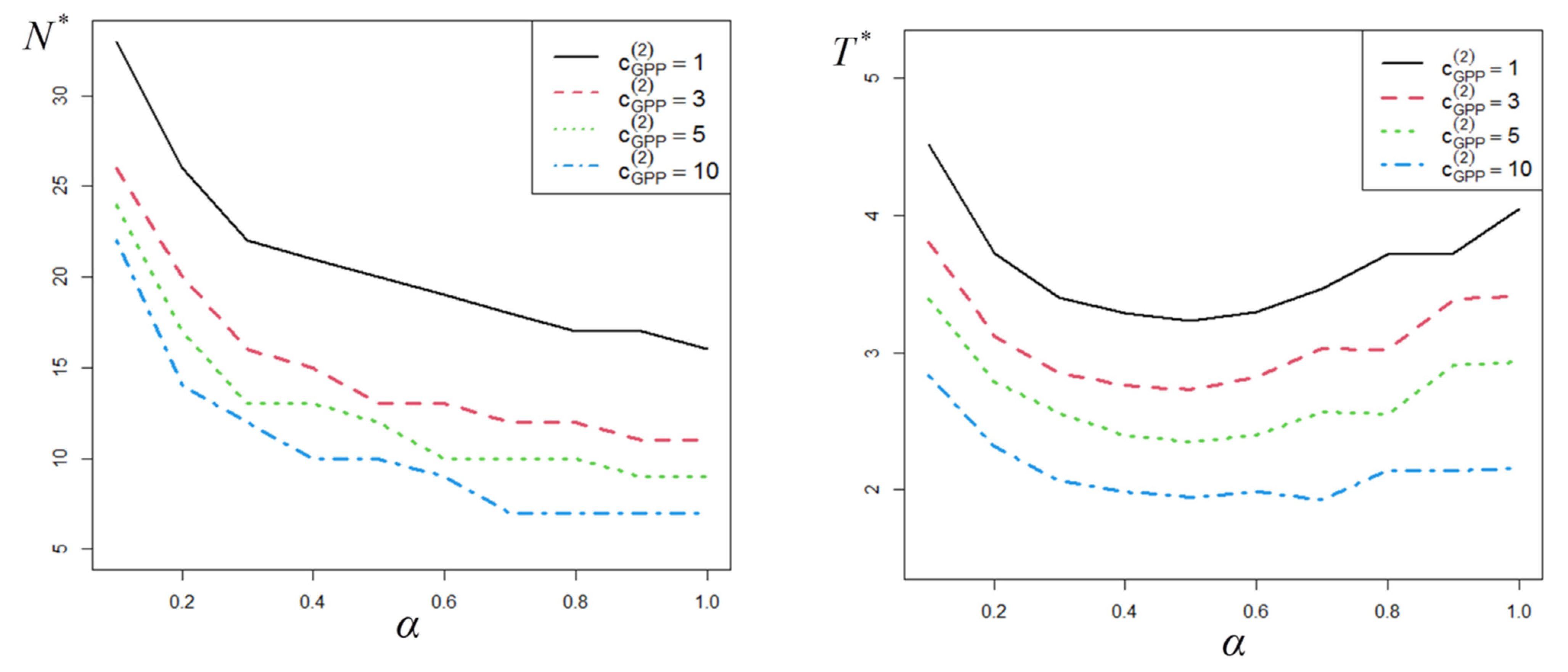
The graphs for the optimal
and
with respect to the value of
are given in
Figure 1 and
Figure 2. As
or
increases, the system should be replaced earlier and thus the corresponding curves are ordered. As
increases, the mean length of the renewal cycle
should be smaller and thus
and
initially decreases. However, when
is larger, the replacement should be made mainly based on the number of failures
(this follows from the form of stochastic intensities in Definition 3) and the role of
should be weaker. Due to this effect,
is increasing when
is increasing.
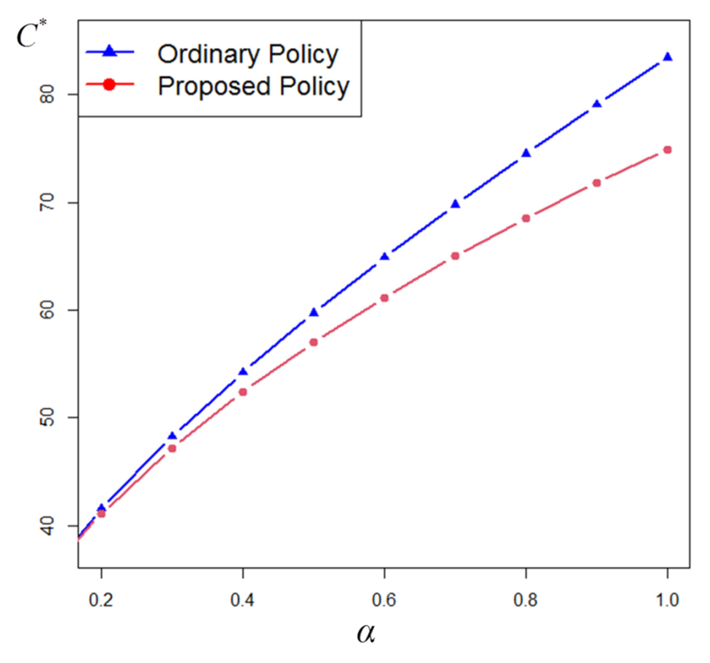
In
Figure 3, the minimum expected cost rates of the two policies for different values of
are presented. The superiority of the proposed replacement policy is clearly seen.
5. Concluding Remarks
In reliability modeling and analysis, the assumption of independence of components in a system is usually made for simplicity and convenience of stochastic description. However, most often, the failures in two or more parts in a system are statistically dependent. Furthermore, in practice, a failure of one part in a system often causes additional stress or damage to the remaining parts, which results in a worse condition of a system than it had just prior this failure. Even a minimal repair of the failed component results in a worse-than-minimal repair of a system in this case.
To model the described practical setting, we employ the bivariate generalized Polya process, which corresponds to the dependent worse-than-minimal repair process. Under these assumptions, a new bivariate preventive maintenance policy based on two parameters (age and operational history) has been proposed and discussed. The corresponding long-run average cost rate has been derived and the optimal replacement policies are investigated and illustrated numerically.
Our mathematical study has a clear practical application in the field of the PM modeling. Along with optimal maintenance, in the future research, the proposed concept of dependent worse-than-minimal repair processes could be used also for describing other reliability properties of repairable systems, such as stationary and non-stationary availability.
As far as we know, our study is the first to apply the dependent bivariate or multivariate counting processes to modeling the multivariate failure processes for stochastic description of repairable systems. Some new stochastic properties of these processes have been derived and the corresponding optimal bivariate preventive maintenance policy with two decision parameters (age and operational history) has been proposed. The latter is another novel feature of the study. Thus, development and application of the new mathematical models for modeling PM with the worse-than-minimal repair can be considered as the main contribution of the paper.
The developed approach and obtained results provide the tools for more adequate stochastic description of real systems with dependent components and worse-than-minimal repair. Neglecting these real-life properties can result in substantial discrepancies in reliability estimates and PM schedules of systems, along with higher costs of maintenance.
The implications of some assumptions in the study should be also addressed in future research. In the multivariate setting, it is also interesting to consider the case when some components undergo minimal repair, whereas others undergo worse-than-minimal repair.


