Multi-View Graph Clustering by Adaptive Manifold Learning

Abstract

Graph-oriented methods have been widely adopted in multi-view clustering because of their efficiency in learning heterogeneous relationships and complex structures hidden in data. However, existing methods are typically investigated based on a Euclidean structure instead of a more suitable manifold topological structure. Hence, it is expected that a more suitable manifold topological structure will be adopted to carry out intrinsic similarity learning. In this paper, we explore the implied adaptive manifold for multi-view graph clustering. Specifically, our model seamlessly integrates multiple adaptive graphs into a consensus graph with the manifold topological structure considered. We further manipulate the consensus graph with a useful rank constraint so that its connected components precisely correspond to distinct clusters. As a result, our model is able to directly achieve a discrete clustering result without any post-processing. In terms of the clustering results, our method achieves the best performance in 22 out of 24 cases in terms of four evaluation metrics on six datasets, which demonstrates the effectiveness of the proposed model. In terms of computational performance, our optimization algorithm is generally faster or in line with other state-of-the-art algorithms, which validates the efficiency of the proposed algorithm.

1. Introduction

In real scenarios, since data typically originates from various sources or consists of different features, a large amount of multi-view data emerges. For example, an object can be described by audio, images, video, and text; news can also be written in different languages [1]. Since the majority of the data is unlabeled, multi-view clustering, which combines the latent information from multiple views and separates the data into different categories [2,3], has become a significant application [4,5,6].

Graph-oriented learning is an efficient approach for modeling heterogeneous relationships and complex structures hidden in data and therefore has been widely adopted in multi-view clustering [7,8,9]. Among them, multi-view clustering based on the adaptive neighbor technique [10], which conducts local manifold structure learning and clustering simultaneously, has been widely utilized with superior performance. The method in [11] learns an optimized graph for each view by assigning adaptive neighbors and then integrates these graphs into a global graph in a well-designed way. To allocate each data sample to the most appropriate cluster and guarantee consistency across views, the method in [12] proposes to make all views share the same similarity matrix. The method in [13,14] learns a similarity graph for each view, and an automated weighting strategy is then adopted to combine the different views efficiently into a unified one. Since all samples in separate views have the same cluster structure, the method in [15] exploits the shared information derived from the links between the different views to obtain a better consensus clustering result. Instead of constructing a similarity graph in the original feature space, the method in [16] learns the critical graph in a spectral embedding space to eliminate the disturbance of noise and redundant information. In addition, the adaptive neighbor technique has been effectively applied to the field of incomplete multi-view clustering [17]. At the same time, there are methods designed to solve the clustering task [18,19].

Although these methods have demonstrated excellent performance, they typically work on Euclidean space and ignore the manifold topological structure, which is crucial for clustering data in the manifold. In this paper, we explicitly explore the manifold topological structure across multiple adaptive graphs by learning a consensus graph. We further manipulate the consensus graph with a useful rank constraint so that its connected components precisely correspond to distinct clusters. As a result, our model is able to directly achieve the discrete clustering result without any post-processing. Our model seamlessly accomplishes three subtasks: It constructs an adaptive graph for each view, integrates the multiple adaptive graphs into a consensus graph with the manifold topological structure considered, and allocates the discrete cluster label for each sample. By leveraging the interactions between these three subtasks in a unified framework, each subtask is iteratively boosted in a mutual reinforcement manner. An iterative updating algorithm is introduced to solve the optimization problem. Experiments on several real-world datasets demonstrate the effectiveness of the proposed model, compared to the state-of-the-art competitors, in terms of four widely used clustering evaluation metrics.

The main contributions of this work are summarized as follows:

• The proposed multi-view graph clustering method, for the first time to the best of our knowledge, explores the topological manifold structure from multiple adaptive graphs such that the topological relevance across multiple views can be explicitly detected.
• Essentially as an end-to-end single-stage learning paradigm, our model seamlessly achieves three subtasks: It constructs the adaptive graphs for each view, explores the topological manifold structure across multiple graphs, and allocates the discrete cluster label for each sample.
• An iterative updating algorithm is carefully designed to solve the optimization problem. Experiments on several benchmark datasets demonstrate the effectiveness of the proposed model.

The remainder of this paper is as follows: In Section 2, we introduce the preliminary work. Section 3 describes the model in detail proposed in this paper. Section 4 introduces the solution and optimization algorithm of the model. Section 5 verifies the validity of the model proposed in this paper through experiments. We conclude the paper in Section 6.

Notations. Throughout this paper, a boldface uppercase letter, e.g., $\mathbf{A}$, denotes a matrix. ${\mathbf{a}}_i$ and $a_{ij}$ represent the i-th column and the $ij$-th element of $\mathbf{A}$, respectively. ${∥·∥}_F$ denotes the Frobenius norm, and $\mathbf{1}$ is a column vector with all its elements being 1. $\mathbf{I}$ represents the identity matrix with proper size.

2. Preliminary Work

Previous works have proven that real-world data are usually sampled from a nonlinear low-dimensional manifold that is embedded in high-dimensional ambient space [20,21,22]. Thus, it is beneficial to reveal the manifold structure implied within the data to boost the corresponding learning performance.

To accurately measure the intrinsic similarity relationships of crowds, the authors in [23] explored the topological relationship between individuals by using a propagation-based manifold learning method. It aims to uncover the topological relevance such that the manifold topological structure can be explicitly considered. There is a simple and intuitive assumption for this consideration: the topological connectivities between distinct individuals could be propagated from near to far. In other words, the spatial similarity between two individuals may be low, but their topological relevance to each other would be high if they are linked by consecutive neighbors. Instead of only making use of the Euclidean structure, it is expected that a more suitable manifold topological structure will be adopted to carry out intrinsic similarity learning. 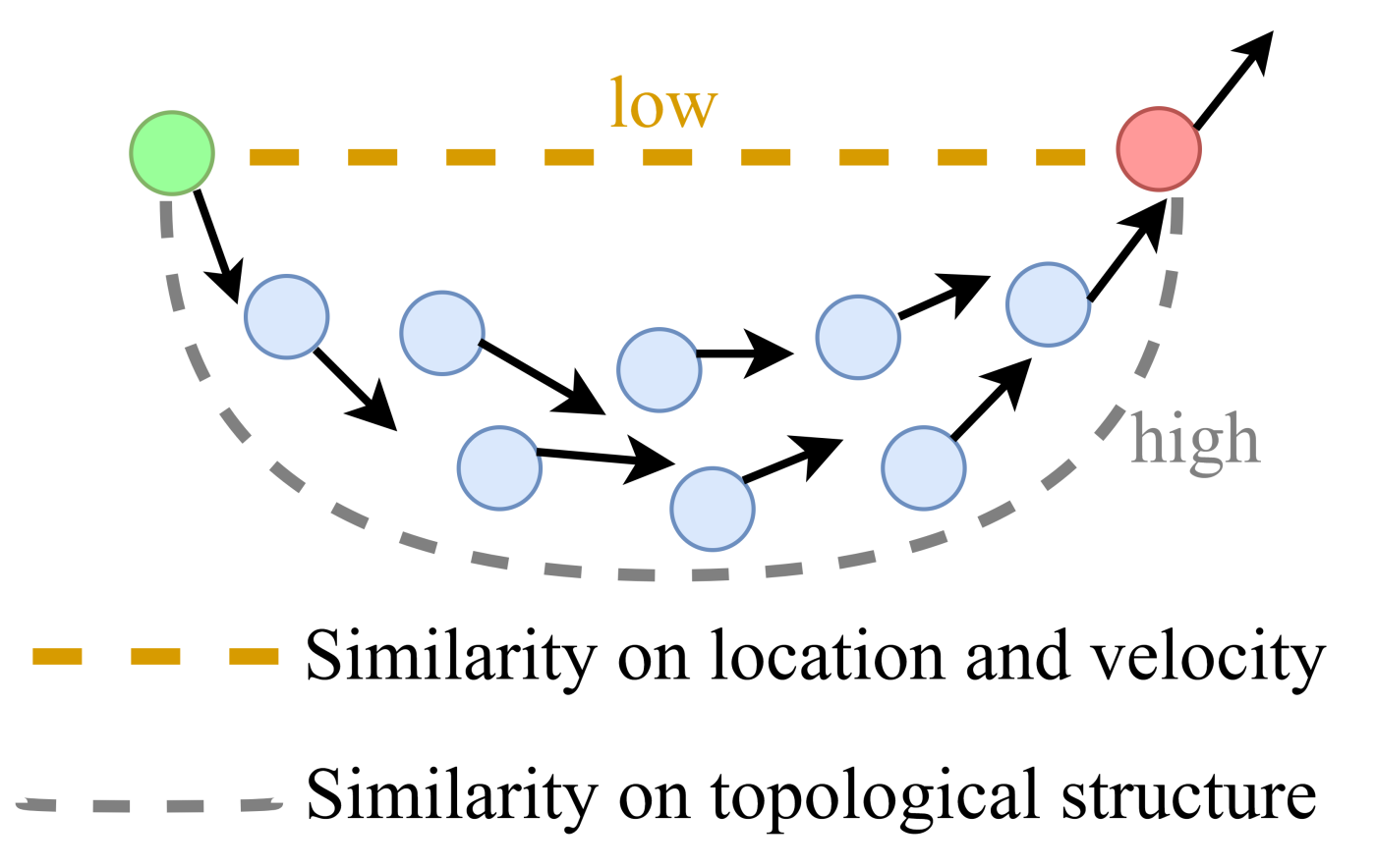Figure 1 visualizes the manifold topological structure learning procedure. As we can see, though the green and red samples have low similarity in terms of spatial location and velocity, they are closely connected to each other considering the high topological relevance between them. That is to say, if two samples maintain a high consistency, their topological relevance to any other sample should be similar.

Suppose a predefined similarity graph $\mathbf{Z}=\left[z_{ij}\right]\in {\mathbb{R}}^{n\times n}$ that depicts the intrinsic similarity relationships of data $\mathbf{X}\in {\mathbb{R}}^{d\times n}$ with n samples and d features. Based on the assumption that data samples with large similarity share similar topological relevance to any other sample, the authors in [23] extract the topological relationship of data samples by solving the following problem:

$$\begin{array}{c}\underset{\mathbf{S}}{\mathbf{min}}\frac{1}{2}{\displaystyle \sum _{i,j,k=1}^n}{z}_{ij}{\left(s_{ki}-s_{kj}\right)}^2+\beta {∥\mathbf{S}-\mathbf{I}∥}_F^2,\end{array}$$

(1)

where $\beta$ is a balance parameter, $\mathbf{S}$ is the target topological relationship matrix, and $s_{ij}$ denotes the data sample j’s topological relevance to i. The first term in Equation (1) is a smoothness constraint that guarantees that the data samples j and k share a similar topological relationship with sample i if j and k are similar. The second term is a fitting constraint that avoids the trivial solution. Based on Equation (1), the topological consistency is propagated through neighbors with high similarities, and the distant data samples will maintain a close relationship if they are linked by consecutive neighbors. Finally, we can search the topological relationship matrix $\mathbf{S}$ by solving the problem defined in Equation (1).

Note that the similarity graph $\mathbf{Z}$ involved in Equation (1) is a fixed graph that might not be optimal for subsequent learning. More often, it is expected a similarity graph will be automatically learned from the original data. To do so, the method described in [10] was proposed to automatically learn a similarity graph for clustering tasks by assigning the adaptive and optimal neighbors for each data sample based on the local connectivity. It is based on a natural assumption that the data samples with a smaller distance should have a larger probability of being neighbors. Instead of a predefined similarity graph, an adaptive graph can be automatically learned by solving the problem as follows:

$$\begin{array}{c}\underset{\mathbf{Z}}{min}{\displaystyle \sum _{i,j=1}^n}\left({∥{\mathbf{x}}_i-{\mathbf{x}}_j∥}_2^2{z}_{ij}+\alpha z_{ij}^2\right)\\ \mathrm{s}.\mathrm{t}.z_{ij}\ge 0,{\mathbf{z}}_i^T\mathbf{1}=1,\end{array}$$

(2)

where $\alpha$ is a trade-off parameter and can be determined according to the number of adaptive neighbors [10].

Let $\{{\mathbf{X}}^{\left(1\right)},\dots ,{\mathbf{X}}^{\left(m\right)}|{\mathbf{X}}^{\left(v\right)}\in {\mathbb{R}}^{n\times d_v}\}$ be a multi-view dataset with m views and $d_v$ features for the v-th view. Equation (2) is easily extended to a multi-view formulation as

$$\begin{array}{c}\underset{{\mathbf{Z}}^{\left(v\right)}}{min}{\displaystyle \sum _{v=1}^m}{\displaystyle \sum _{i,j=1}^n}\left({∥{\mathbf{x}}_i^{\left(v\right)}-{\mathbf{x}}_j^{\left(v\right)}∥}_2^2{z}_{ij}^{\left(v\right)}+\alpha {\left(z_{ij}^{\left(v\right)}\right)}^2\right)\\ \mathrm{s}.\mathrm{t}.z_{ii}^{\left(v\right)}\ge 0,{\left({\mathbf{z}}_i^{\left(v\right)}\right)}^T\mathbf{1}=1,\end{array}$$

(3)

where ${\mathbf{Z}}^{\left(v\right)}$ denotes the adaptive graph learned from the v-th view.

3. The Proposed Model

Note that the formulation in Equation (1) has several drawbacks. First, if a data sample is connected with many similar neighbors, it will largely affect the objective value. Hence, it is required that a normalized version of Equation (1) be designed, such that each sample is treated equally. That is to say, a data sample with too many connections would dominate the objective function. The normalization has two main purposes: (1) it ensures that each sample is treated equally; (2) it is equivalent to a sparse constraint, i.e., a $l_1$-norm on a similarity graph. Second, the learned $\mathbf{S}$ does not contain the explicit cluster structures, so a subsequent postprocessing step is needed to output the final discrete clustering results. It is preferred that the similarity graph and cluster structure are learned simultaneously. It sounds unrealistic to achieve such a pure structured graph. Fortunately, we can tackle this problem with a useful rank constraint. Taking the above concerns into consideration, Equation (1) can be upgraded to

$$\begin{array}{c}\underset{\mathbf{S}}{min}\frac{1}{2}{\displaystyle \sum _{i,j,k=1}^n}{z}_{ij}{\left(\frac{s_{ki}}{\sqrt{d_{ii}}}-\frac{s_{kj}}{\sqrt{d_{jj}}}\right)}^2+\beta {∥\mathbf{S}-\mathbf{I}∥}_F^2,\\ \mathrm{s}.\mathrm{t}.{\mathbf{s}}_i^T\mathbf{1}=1,s_{ij}\ge 0,rank\left({\mathbf{L}}_S\right)=n-c,\end{array}$$

(4)

where $\mathbf{D}=\left[d_{ij}\right]\in {\mathbb{R}}^{n\times n}$ is the degree matrix of $\mathbf{Z}$, ${\mathbf{L}}_S$ is the Laplacian matrix of $\mathbf{S}$, and $rank\left({\mathbf{L}}_S\right)=n-c$ is a rank constraint that guarantees that $\mathbf{S}$ contains exactly c connected components (c is the cluster number of data). The rank constraint has been successfully used to achieve a clear cluster structure [10,24]. Note that, unlike Equation (1), here we constrain the sum of each row of $\mathbf{S}$ to be one, and all elements of $\mathbf{S}$ are nonnegative. Finally, a structured target graph $\mathbf{S}$ that reveals the topological relevance can be acquired by solving Equation (4).

In this paper, we extract the topological relevance from multiple adaptive graphs such that the manifold topological structure can be explicitly detected for the clustering task. Combining Equation (4) and Equation (3), our new multi-view graph clustering model can be formulated as

$$\begin{array}{c}\underset{{\mathbf{Z}}^{\left(v\right)},\mathbf{S}}{min}{\displaystyle \sum _{v=1}^m}{\displaystyle \sum _{i,j=1}^n}\left({∥{\mathbf{x}}_i^{\left(v\right)}-{\mathbf{x}}_j^{\left(v\right)}∥}_2^2{z}_{ij}^{\left(v\right)}+\alpha {\left(z_{ij}^{\left(v\right)}\right)}^2\right)+\\ \frac{1}{2}{\displaystyle \sum _{v=1}^m}{\mu }^{\left(v\right)}{\displaystyle \sum _{i,j,k=1}^n}{z}_{ij}^{\left(v\right)}{\left(\frac{s_{ki}}{\sqrt{d_{ii}^{\left(v\right)}}}-\frac{s_{kj}}{\sqrt{d_{jj}^{\left(v\right)}}}\right)}^2+\beta {∥\mathbf{S}-\mathbf{I}∥}_F^2\\ \mathrm{s}.\mathrm{t}.{\left({\mathbf{z}}_i^{\left(v\right)}\right)}^T\mathbf{1}=1,z_{ij}^{\left(v\right)}\ge 0,\\ {\mathbf{s}}_i^T\mathbf{1}=1,s_{ij}\ge 0,rank\left({\mathbf{L}}_S\right)=n-c,\end{array}$$

(5)

where ${\mu }^{\left(v\right)}$ denotes the weight of the v-th view and can be determined by an inverse distance weighting strategy, i.e.,

$$\begin{array}{c}{\mu }^{\left(v\right)}=1/2\sqrt{{\displaystyle \sum _{i,j,k=1}^n}{z}_{ij}^{\left(v\right)}{\left(\frac{s_{ki}}{\sqrt{d_{ii}^{\left(v\right)}}}-\frac{s_{kj}}{\sqrt{d_{jj}^{\left(v\right)}}}\right)}^2}.\end{array}$$

(6)

Note that Equation (6) is essentially a kind of auto-weighted strategy, which has been widely utilized in previous works [7,25,26]. To further verify the effect of an auto-weighting strategy, we will conduct an ablation study in a later section.

Note that, if we denote ${\sigma }_i\left({\mathbf{L}}_S\right)$ as the i-th smallest eigenvalue of ${\mathbf{L}}_S$, the rank constraint $rank\left({\mathbf{L}}_S\right)=n-c$ would be satisfied if ${\sum }_{i=1}^k{\sigma }_i\left({\mathbf{L}}_S\right)=0$ since ${\mathbf{L}}_S$ is a positive semidefinite matrix. According to Ky Fan’s Theorem [27] that ${\sum }_{i=1}^c{\sigma }_i\left({\mathbf{L}}_S\right)={min}_{\mathbf{F}}\mathrm{Tr}\left({\mathbf{F}}^T{\mathbf{L}}_S\mathbf{F}\right)$, we can incorporate the rank constraint term into the objective function, and finally we arrive at

$$\begin{array}{c}\underset{{\mathbf{Z}}^{\left(v\right)},\mathbf{S},\mathbf{F}}{min}{\displaystyle \sum _{v=1}^m}{\displaystyle \sum _{i,j=1}^n}\left({∥{\mathbf{x}}_i^{\left(v\right)}-{\mathbf{x}}_j^{\left(v\right)}∥}_2^2{z}_{ij}^{\left(v\right)}+\alpha {\left(z_{ij}^{\left(v\right)}\right)}^2\right)\\ +\frac{1}{2}{\displaystyle \sum _{v=1}^m}{\mu }^{\left(v\right)}{\displaystyle \sum _{i,j,k=1}^n}{z}_{ij}^{\left(v\right)}{\left(\frac{s_{ki}}{\sqrt{d_{ii}^{\left(v\right)}}}-\frac{s_{kj}}{\sqrt{d_{jj}^{\left(v\right)}}}\right)}^2+\beta {∥\mathbf{S}-\mathbf{I}∥}_F^2+2\gamma \mathrm{Tr}\left({\mathbf{F}}^T{\mathbf{L}}_S\mathbf{F}\right)\\ \mathrm{s}.\mathrm{t}.{\left({\mathbf{z}}_i^{\left(v\right)}\right)}^T\mathbf{1}=1,z_{ij}^{\left(v\right)}\ge 0,{\mathbf{s}}_i^T\mathbf{1}=1,s_{ij}\ge 0,\\ \mathbf{F}\in {\mathbb{R}}^{n\times c},{\mathbf{F}}^T\mathbf{F}=\mathbf{I},\end{array}$$

(7)

where $\gamma$ is a self-adjusted parameter, and $\mathbf{F}$ denotes the cluster indicator matrix. When $\gamma$ is large enough, the optimal solution $\mathbf{S}$ for Equation (7) will enforce the last term $\mathrm{Tr}\left({\mathbf{F}}^T{\mathbf{L}}_S\mathbf{F}\right)$, i.e., ${\sum }_{i=1}^c{\sigma }_i\left({\mathbf{L}}_S\right)$, to be zero. Thus, the constraint $rank\left({\mathbf{L}}_S\right)=n-c$ in Equation (7) could be satisfied. Moreover, according to [26], $\gamma$ can be tuned in a heuristic way: initialize $\gamma$ to a positive value (e.g., $\gamma =10$) and we then automatically halve (i.e., $\gamma \leftarrow \frac{\gamma }{2}$) or double (i.e., $\gamma \leftarrow 2\ast \gamma$) it when its number of connected components is greater or smaller than the cluster number c in each iteration. In this way, the target graph $\mathbf{S}$ will be modified until it contains precisely c connected components.

4. Optimization

Since the optimization problem in Equation (7) is not jointly convex in all variables, we optimize it with respect to one variable while fixing other variables.

4.1. Update ${\mathbf{Z}}^{\left(v\right)}$

The optimization problem for ${\mathbf{Z}}^{\left(v\right)}$ can be stated as

$$\begin{array}{c}\underset{{\mathbf{Z}}^{\left(v\right)}}{min}{\displaystyle \sum _{v=1}^m}{\displaystyle \sum _{i,j=1}^n}\left({∥{\mathbf{x}}_i^{\left(v\right)}-{\mathbf{x}}_j^{\left(v\right)}∥}_2^2{z}_{ij}^{\left(v\right)}+\alpha {\left(z_{ij}^{\left(v\right)}\right)}^2\right)+\frac{1}{2}{\displaystyle \sum _{v=1}^m}{\mu }^{\left(v\right)}{\displaystyle \sum _{i,j,k=1}^n}{z}_{ij}^{\left(v\right)}{\left(\frac{s_{ki}}{\sqrt{d_{ii}^{\left(v\right)}}}-\frac{s_{kj}}{\sqrt{d_{jj}^{\left(v\right)}}}\right)}^2\\ \mathrm{s}.\mathrm{t}.{\left({\mathbf{z}}_i^{\left(v\right)}\right)}^T\mathbf{1}=1,z_{ij}^{\left(v\right)}\ge 0.\end{array}$$

(8)

Since Equation (8) is independent for different v, for a specific v, we need to solve

$$\begin{array}{c}\underset{{\mathbf{Z}}^{\left(v\right)}}{min}{\displaystyle \sum _{i,j=1}^n}\left(h_{ij}^x{z}_{ij}^{\left(v\right)}+\alpha {\left(z_{ij}^{\left(v\right)}\right)}^2+\frac{1}{2}{\mu }^{\left(v\right)}{h}_{ij}^s{z}_{ij}^{\left(v\right)}\right)\\ \mathrm{s}.\mathrm{t}.{\left({\mathbf{z}}_i^{\left(v\right)}\right)}^T\mathbf{1}=1,z_{ij}^{\left(v\right)}\ge 0,\end{array}$$

(9)

where $h_{ij}^x={∥{\mathbf{x}}_i^{\left(v\right)}-{\mathbf{x}}_j^{\left(v\right)}∥}_2^2$, and $h_{ij}^s={∥\frac{{\mathbf{s}}_i}{\sqrt{d_{ii}^{\left(v\right)}}}-\frac{{\mathbf{s}}_j}{\sqrt{d_{jj}^{\left(v\right)}}}∥}_2^2$. Note that, for each i, Equation (9) can be transformed into a compact vector form as

$$\begin{array}{c}\underset{{\left({\mathbf{z}}_i^{\left(v\right)}\right)}^T\mathbf{1}=1,z_{ij}^{\left(v\right)}\ge 0}{min}{∥{\mathbf{z}}_i^{\left(v\right)}+\frac{1}{2\alpha }{\mathbf{h}}_i∥}_2^2,\end{array}$$

(10)

where ${\mathbf{h}}_i$ is a vector with its j-th element being

$$\begin{array}{c}{h}_{ij}=h_{ij}^x+\frac{1}{2}{\mu }^{\left(v\right)}{h}_{ij}^s.\end{array}$$

(11)

Note that Equation (10) has a closed-form solution according to [28].

4.2. Update $\mathbf{S}$

The optimization problem with respect to $\mathbf{S}$ can be denoted as

$$\begin{array}{c}\underset{\mathbf{S}}{min}\frac{1}{2}{\displaystyle \sum _{v=1}^m}{\mu }^{\left(v\right)}{\displaystyle \sum _{i,j,k=1}^n}{z}_{jk}^{\left(v\right)}{\left(\frac{s_{ij}}{\sqrt{d_{jj}^{\left(v\right)}}}-\frac{s_{ik}}{\sqrt{d_{kk}^{\left(v\right)}}}\right)}^2+\beta {∥\mathbf{S}-\mathbf{I}∥}_F^2+2\gamma \mathrm{Tr}\left({\mathbf{F}}^T{\mathbf{L}}_S\mathbf{F}\right)\\ \mathrm{s}.\mathrm{t}.{\mathbf{s}}_i^T\mathbf{1}=1,s_{ij}\ge 0.\end{array}$$

(12)

It is obvious that Equation (12) can be rewritten as

$$\begin{array}{c}\underset{\mathbf{S}}{min}{\displaystyle \sum _{i=1}^n}\left\{{\displaystyle \sum _{v=1}^m}\frac{1}{2}{\mu }^{\left(v\right)}{\displaystyle \sum _{j,k=1}^n}{z}_{jk}^{\left(v\right)}{\left(\frac{s_{ij}}{\sqrt{d_{jj}^{\left(v\right)}}}-\frac{s_{ik}}{\sqrt{d_{kk}^{\left(v\right)}}}\right)}^2+\beta {\displaystyle \sum _{j=1}^n}{\left(s_{ij}-e_{ij}\right)}^2+\gamma {\displaystyle \sum _{j=1}^n}{∥{\mathbf{f}}_i-{\mathbf{f}}_j∥}_2^2{s}_{ij}\right\}\\ \mathrm{s}.\mathrm{t}.{\mathbf{s}}_i^T\mathbf{1}=1,s_{ij}\ge 0,\end{array}$$

(13)

where $e_{ij}$ is the $ij$-th element of the identity matrix $\mathbf{I}$.

Note that Equation (13) is independent for different i, so we have

$$\begin{array}{c}\underset{s_{ij}\ge 0,{\mathbf{s}}_i^T\mathbf{1}=1}{min}{\mathbf{s}}_i^T\left({\displaystyle \sum _{v=1}^m}{\mu }^{\left(v\right)}\left(\mathbf{I}-{{\mathbf{D}}^{\left(v\right)}}^{-\frac{1}{2}}{\mathbf{Z}}^{\left(v\right)}{{\mathbf{D}}^{\left(v\right)}}^{-\frac{1}{2}}\right)\right){\mathbf{s}}_i+\beta {∥{\mathbf{s}}_i-{\mathbf{e}}_i∥}_2^2+{\mathbf{s}}_i^T{\mathbf{u}}_i,\end{array}$$

(14)

where ${\mathbf{u}}_i$ represents a vector with its j-th element $u_{ij}=\gamma {∥{\mathbf{f}}_i-{\mathbf{f}}_j∥}_2^2$.

Denote $\mathbf{A}={\sum }_{v=1}^m{\mu }^{\left(v\right)}\left(\mathbf{I}-{{\mathbf{D}}^{\left(v\right)}}^{-\frac{1}{2}}{\mathbf{Z}}^{\left(v\right)}{{\mathbf{D}}^{\left(v\right)}}^{-\frac{1}{2}}\right)+\beta \mathbf{I}$ and $\mathbf{b}=2\beta {\mathbf{e}}_i-{\mathbf{u}}_i$. Equation (14) can then be stated as

$$\begin{array}{c}\underset{s_{ij}\ge 0,{\mathbf{s}}_i^T\mathbf{1}=1}{min}{\mathbf{s}}_i^T\mathbf{A}{\mathbf{s}}_i-{\mathbf{s}}_i^T\mathbf{b}.\end{array}$$

(15)

Equation (15) turns out to be a quadratic convex optimization problem, which can be tackled by the augmented Lagrangian multiplier (ALM) strategy [29]. According to the ALM, the counterpart of Equation (15) is defined as

$$\begin{array}{c}\underset{s_{ij}\ge 0,{\mathbf{s}}_i^T\mathbf{1}=1,\mathbf{p}={\mathbf{s}}_i}{min}{\mathbf{s}}_i^T\mathbf{A}\mathbf{p}-{\mathbf{s}}_i^T\mathbf{b},\end{array}$$

(16)

where $\mathbf{p}$ is the Lagrangian multiplier. Thus, the augmented Lagrangian function of Equation (16) can be represented as

$$\begin{array}{c}\underset{s_{ij}\ge 0,{\mathbf{s}}_i^T\mathbf{1}=1,\mathbf{p}}{min}{\mathbf{s}}_i^T\mathbf{A}\mathbf{p}-{\mathbf{s}}_i^T\mathbf{b}+\frac{\eta }{2}{∥{\mathbf{s}}_i-\mathbf{p}+\frac{1}{\eta }\mathbf{q}∥}_2^2,\end{array}$$

(17)

where $\eta$ and $\mathbf{q}$ are the corresponding penalty coefficient and parameter, respectively.

To solve Equation (17), we can update $\mathbf{p}$ and ${\mathbf{s}}_i$ iteratively:

(1) Update $\mathbf{p}$ with a fixed ${\mathbf{s}}_i$. The Lagrange function of Equation (17) with respect to $\mathbf{p}$ can be formulated as

$$\begin{array}{c}{\mathcal{L}}_{\mathbf{p}}={\mathbf{s}}_i^T\mathbf{A}\mathbf{p}+\frac{\eta }{2}{∥{\mathbf{s}}_i-\mathbf{p}+\frac{1}{\eta }\mathbf{q}∥}_2^2.\end{array}$$

(18)

Taking the derivative of ${\mathcal{L}}_{\mathbf{p}}$ with respect to $\mathbf{p}$ and setting the derivative to zero, i.e.,

$$\begin{array}{c}\frac{\partial {\mathcal{L}}_{\mathbf{p}}}{\partial \mathbf{p}}=0,\end{array}$$

(19)

we obtain the following solution:

$$\begin{array}{c}\mathbf{p}={\mathbf{s}}_i-\frac{1}{\eta }\left({\mathbf{A}}^T{\mathbf{s}}_i+\mathbf{q}\right).\end{array}$$

(20)

(2) Update ${\mathbf{s}}_i$ with a fixed $\mathbf{p}$. The Lagrange function of Equation (17) with respect to ${\mathbf{s}}_i$ is

$$\begin{array}{c}\underset{s_{ij}\ge 0,{\mathbf{s}}_i^T\mathbf{1}=1}{min}{∥{\mathbf{s}}_i-\mathbf{p}+\frac{1}{\eta }\mathbf{q}+\frac{\mathbf{A}\mathbf{p}-\mathbf{b}}{\eta }∥}_2^2,\end{array}$$

(21)

which has a similar form to Equation (10) and thus can be solved effectively. Note that $\eta$ is exaggerated increasingly during each iteration, and $\mathbf{q}$ can be updated by $\mathbf{q}\leftarrow \mathbf{q}+\eta \left({\mathbf{s}}_i-\mathbf{p}\right)$. The optimization routine for Equation (17) is outlined in Algorithm 1.

Algorithm 1: Algorithm to solve Equation (17).

Require: a nonzero matrix A and a nonzero vector b.

Set 1 < ρ < 2, initialize η > 0, q.

Ensure: S.

1: repeat

2:  Update p according to (20).

3:  Update si according to (21).

4:  Update η ← ρη.

5:  Update q ← q + η (si − p).

1: until converge

4.3. Update F

The optimal solution of $\mathbf{F}$ can be searched by solving

$$\begin{array}{c}\underset{\mathbf{F}\in {\mathbb{R}}^{n\times c},{\mathbf{F}}^T\mathbf{F}=\mathbf{I}}{min}\mathrm{Tr}\left({\mathbf{F}}^T{\mathbf{L}}_S\mathbf{F}\right),\end{array}$$

(22)

which is a classical problem in spectral theory, and the solution is formed by the c eigenvectors of ${\mathbf{L}}_S$ corresponding to the c smallest eigenvalues.

Up to now, the overall algorithm to solve the proposed objective function in Equation (7) is summarized in Algorithm 2. We will provide the time complexity and convergence analysis of Algorithm 2 in a later section.

Algorithm 2: The algorithm for our model.

Require: multi-view data $\{{\mathbf{X}}^{\left(1\right)},{\mathbf{X}}^{\left(2\right)},\dots ,{\mathbf{X}}^{\left(m\right)}\}$ with m views, cluster number c, parameters $\alpha$ and $\beta$.

Initialize the weight of each view ${\mu }^{\left(v\right)}=\frac{1}{m}$.

Initialize ${\mathbf{Z}}^{\left(v\right)}$ for each view by (2).

Initialize the consensus graph $\mathbf{S}={\sum }_{v=1}^m{\mu }^{\left(v\right)}{\mathbf{Z}}^{\left(v\right)}$.

Ensure: The target $\mathbf{S}\in {\mathbb{R}}^{n\times n}$ with exactly c connected components, and the cluster indicator matrix F.

1: repeat

2:  Update ${\mathbf{Z}}^{\left(v\right)}$ according to Equation (10).

3:  Update S by Algorithm 1.

4:  Update F according to Equation (22).

5:  Update ${\mu }^{\left(v\right)}$ according to Equation (6).

6: Until converge

4.4. Time Complexity Analysis

As shown in Algorithm 2, there are four steps that mainly determine the complexity of our model. Recall that n, m, and c denote the number of data points, views, and clusters, respectively. t denotes the number of iterations. We summarize the computational complexity of each step in

Table 1. Details of computational complexity.

Steps	Calculation	Complexity
Equation (10)	update ${\mathbf{Z}}^{\left(v\right)}$	$\mathcal{O}\left(nmc\right)$
Algorithm 1	update $\mathbf{S}$	$\mathcal{O}\left(n{m}^{2}c+nmc\right)$
Equation (22)	c eigenvectors of ${\mathbf{L}}_S$	$\mathcal{O}\left(n^{2}c\right)$
Equation (6)	view weight ${\mu }^{\left(v\right)}$	$\mathcal{O}\left(n^{2}mc\right)$
Total	$\mathcal{O}\left(n^{2}t\right)$

.

In practice, we have $m\ll n$ and $c\ll n$, so the overall complexity is $\mathcal{O}\left(n^{2}t\right)$, which is in line with the classical graph-based methods and hence is acceptable.

4.5. Convergence Analysis

In Algorithm 2, we can obtain the closed-form solutions with respect to ${\mathbf{Z}}^{\left(v\right)}$, ${\mu }^{\left(v\right)}$, and $\mathbf{F}$, as described in the main paper. ALM optimization theory [30] guarantees that the iterations will make the optimization process converge. In a word, the updating of variables ${\mathbf{Z}}^{\left(v\right)}$, ${\mu }^{\left(v\right)}$, and $\mathbf{F}$ with iterative optimization steps will monotonically decrease toward the lower bound of the objective function in (7). Hence, we only need to prove the convergence of (12) with respect to $\mathbf{S}$. We will show that our algorithm can find a local optimal solution. Before we prove its convergence, first we introduce an important lemma as follows [31]:

Lemma 1.

For any positive real number q and t, the following inequality holds:

$$\begin{array}{c}\sqrt{q}-\frac{q}{2\sqrt{t}}\le \sqrt{t}-\frac{t}{2\sqrt{t}}.\end{array}$$

Proof. 

It is obvious that the inequality ${(\sqrt{q}-\sqrt{t})}^2\ge 0$, so we have ${(\sqrt{q}-\sqrt{t})}^2\ge 0\Rightarrow q-2\sqrt{qt}+t\ge 0\Rightarrow \sqrt{q}-\frac{q}{2\sqrt{t}}\le \frac{\sqrt{t}}{2}\Rightarrow \sqrt{q}-\frac{q}{2\sqrt{t}}\le \sqrt{t}-\frac{t}{2\sqrt{t}}$ which completes the proof. □

Theorem 1.

In each iteration, the updated $\mathbf{S}$ will monotonically decrease the objective in Equation (12), which generally makes the solution converge to the local optimum of Equation (12).

Proof. 

Suppose the alternatively updated $\mathbf{S}$ is $\tilde{\mathbf{S}}$ in each iteration. By solving Equation (17), we obtain

$$\begin{array}{c}\tilde{\mathbf{S}}=\underset{\mathbf{S}}{\mathrm{arg\; min}}\left\{\frac{1}{2}{\displaystyle \sum _{v=1}^m}{\mu }^{\left(v\right)}{\displaystyle \sum _{i,j,k=1}^n}{z}_{jk}^{\left(v\right)}{\left(\frac{s_{ij}}{\sqrt{d_{jj}^{\left(v\right)}}}-\frac{s_{ik}}{\sqrt{d_{kk}^{\left(v\right)}}}\right)}^2+\beta {∥\mathbf{S}-\mathbf{I}∥}_F^2\right\}.\end{array}$$

According to Equation (6), i.e., ${\mu }^{\left(v\right)}=1/2\sqrt{{\displaystyle \sum _{i,j,k=1}^n}{z}_{jk}^{\left(v\right)}{\left(\frac{s_{ij}}{\sqrt{d_{jj}^{\left(v\right)}}}-\frac{s_{ik}}{\sqrt{d_{kk}^{\left(v\right)}}}\right)}^2}$, we obtain

$$\begin{array}{c}\frac{1}{2}{\displaystyle \sum _{v=1}^m}\frac{{\displaystyle \sum _{i,j,k=1}^n}{z}_{jk}^{\left(v\right)}{\left(\frac{{\tilde{s}}_{ij}}{\sqrt{d_{jj}^{\left(v\right)}}}-\frac{{\tilde{s}}_{ik}}{\sqrt{d_{kk}^{\left(v\right)}}}\right)}^2}{2\sqrt{{\displaystyle \sum _{i,j,k=1}^n}{z}_{jk}^{\left(v\right)}{\left(\frac{s_{ij}}{\sqrt{d_{jj}^{\left(v\right)}}}-\frac{s_{ik}}{\sqrt{d_{kk}^{\left(v\right)}}}\right)}^2}}+\mathcal{G}\left(\tilde{\mathbf{S}}\right)\le \\ \frac{1}{2}{\displaystyle \sum _{v=1}^m}\frac{{\displaystyle \sum _{i,j,k=1}^n}{z}_{jk}^{\left(v\right)}{\left(\frac{s_{ij}}{\sqrt{d_{jj}^{\left(v\right)}}}-\frac{s_{ik}}{\sqrt{d_{kk}^{\left(v\right)}}}\right)}^2}{2\sqrt{{\displaystyle \sum _{i,j,k=1}^n}{z}_{jk}^{\left(v\right)}{\left(\frac{s_{ij}}{\sqrt{d_{jj}^{\left(v\right)}}}-\frac{s_{ik}}{\sqrt{d_{kk}^{\left(v\right)}}}\right)}^2}}+\mathcal{G}\left(\mathbf{S}\right),\end{array}$$

where $\mathcal{G}\left(\mathbf{S}\right)=\beta {∥\mathbf{S}-\mathbf{I}∥}_F^2$.

Based on Lemma 1, we have

$$\begin{array}{c}\frac{1}{2}{\displaystyle \sum _{v=1}^m}\sqrt{{\displaystyle \sum _{i,j,k=1}^n}{z}_{jk}^{\left(v\right)}{\left(\frac{{\tilde{s}}_{ij}}{\sqrt{d_{jj}^{\left(v\right)}}}-\frac{{\tilde{s}}_{ik}}{\sqrt{d_{kk}^{\left(v\right)}}}\right)}^2}-\frac{1}{2}{\displaystyle \sum _{v=1}^m}\frac{{\displaystyle \sum _{i,j,k=1}^n}{z}_{jk}^{\left(v\right)}{\left(\frac{{\tilde{s}}_{ij}}{\sqrt{d_{jj}^{\left(v\right)}}}-\frac{{\tilde{s}}_{ik}}{\sqrt{d_{kk}^{\left(v\right)}}}\right)}^2}{2\sqrt{{\displaystyle \sum _{i,j,k=1}^n}{z}_{jk}^{\left(v\right)}{\left(\frac{s_{ij}}{\sqrt{d_{jj}^{\left(v\right)}}}-\frac{s_{ik}}{\sqrt{d_{kk}^{\left(v\right)}}}\right)}^2}}\\ \le \frac{1}{2}{\displaystyle \sum _{v=1}^m}\sqrt{{\displaystyle \sum _{i,j,k=1}^n}{z}_{jk}^{\left(v\right)}{\left(\frac{s_{ij}}{\sqrt{d_{jj}^{\left(v\right)}}}-\frac{s_{ik}}{\sqrt{d_{kk}^{\left(v\right)}}}\right)}^2}-\frac{1}{2}{\displaystyle \sum _{v=1}^m}\frac{{\displaystyle \sum _{i,j,k=1}^n}{z}_{jk}^{\left(v\right)}{\left(\frac{s_{ij}}{\sqrt{d_{jj}^{\left(v\right)}}}-\frac{s_{ik}}{\sqrt{d_{kk}^{\left(v\right)}}}\right)}^2}{2\sqrt{{\displaystyle \sum _{i,j,k=1}^n}{z}_{jk}^{\left(v\right)}{\left(\frac{s_{ij}}{\sqrt{d_{jj}^{\left(v\right)}}}-\frac{s_{ik}}{\sqrt{d_{kk}^{\left(v\right)}}}\right)}^2}}.\end{array}$$

By summing over the above two equations in the two sides, we obtain

$$\begin{array}{c}\frac{1}{2}{\displaystyle \sum _{v=1}^m}\sqrt{{\displaystyle \sum _{i,j,k=1}^n}{z}_{jk}^{\left(v\right)}{\left(\frac{{\tilde{s}}_{ij}}{\sqrt{d_{jj}^{\left(v\right)}}}-\frac{{\tilde{s}}_{ik}}{\sqrt{d_{kk}^{\left(v\right)}}}\right)}^2}+\mathcal{G}\left(\tilde{\mathbf{S}}\right)\\ \le \frac{1}{2}{\displaystyle \sum _{v=1}^m}\sqrt{{\displaystyle \sum _{i,j,k=1}^n}{z}_{jk}^{\left(v\right)}{\left(\frac{s_{ij}}{\sqrt{d_{jj}^{\left(v\right)}}}-\frac{s_{ik}}{\sqrt{d_{kk}^{\left(v\right)}}}\right)}^2}+\mathcal{G}\left(\mathbf{S}\right),\end{array}$$

which completes the proof. That is, the objective function value will monotonically decrease in each iteration of updating $\mathbf{S}$. □

5. Experiments

To verify the efficiency of our proposed method, we compare it with the following state-of-the-art methods: self-weighted multi-view clustering (SwMC) [7], multi-view learning with adaptive neighbours (MLAN) [12], multi-view clustering via adaptively weighted procrustes (AWP) [32], weighted multi-view spectral clustering (WMSC) [33], multi-view consensus graph clustering (MCGC) [15], consistent and specific multi-view subspace clustering (CSMSC) [34], graph-based multi-view clustering (GMC) [14], consensus one-step multi-view subspace clustering (COMSC) [35], and multi-view clustering via consensus graph learning (CGL) [16].

We conduct the experiments on several prevalent datasets, namely, 3Sources, MSRC, BBCSport, COIL-20, Caltech-7, and Caltech-20. The detailed information of all datasets is as follows: 3Sources (http://mlg.ucd.ie/datasets/3sources.html (accessed on 26 April 2022)) is collected from three news sources, i.e., Reuters, BBC, and The Guardian. There are 948 news articles covering 416 different news stories. Among them, 169 news stories were reported in all three sources, and each story was annotated with one of six topical labels: business, health, politics, entertainment, sport, and technology. MSRC is comprised of 240 images in eight classes. We selected seven classes with each class containing 30 images. For each image, five visual features are extracted for a comprehensive description. BBCSport is a sports news dataset that consists of 544 articles in 5 areas with 2 views. The 2 views are 3183 dimension MTX features and 3203 dimension TERMS features, respectively. COIL-20 is a subset of an object database (http://www.cs.columbia.edu/CAVE/software/softlib/coil-100.php (accessed on 26 April 2022)) that includes 100 categories. Images of each object were taken five degrees apart as the object was rotated on a turntable, and each object has 72 gray images. Each image is described by three types of features. Caltech101 is an object recognition dataset with 101 categories. This dataset is represented by 6 types of features. Following [12], we selected 1474 images within 7 classes (Caltech-7) and 2386 images within 20 classes (Caltech-20).

The specific characteristics of the datasets are given in

Table 2. Characteristics of all datasets.

Data Set	n	m	c	${\mathit{d}}_1$	${\mathit{d}}_2$	${\mathit{d}}_3$	${\mathit{d}}_4$	${\mathit{d}}_5$	${\mathit{d}}_6$
3Sources	169	3	6	3560	3631	3068	–	–	–
MSRC	210	5	7	24	576	512	256	254	–
BBCSport	544	2	5	3183	3203	–	–	–	–
COIL-20	1440	3	20	1024	3304	6750	–	–	–
Caltech-7	1474	6	7	48	40	254	1984	512	928
Caltech-20	2386	6	20	48	40	254	1984	512	928

n, m, and c denote the number of samples, views, and clusters, respectively. d_v denotes the dimensionality of the features in the v-th view.

.

The parameters for comparison algorithms were set according to the recommendations in their corresponding paper. The parameter settings of our model will be introduced later. All algorithms were repeated 10 times, and the average results are presented.

To achieve a comprehensive evaluation, four widely used metrics (clustering accuracy (ACC), normalized mutual information (NMI), purity, and F-score) are adopted in this paper.

5.1. Clustering Results

The clustering performance of different methods on all datasets is reported in

Table 3. Clustering results of all methods on different datasets (%). The best performance is bolded, and the second best performance is underlined.

Dataset	SwMC	MLAN	AWP	WMSC	MCGC	CSMSC	GMC	COMSC	CGL	Ours
ACC
3Sources	39.64	79.88	54.44	57.81	56.80	78.28	69.23	57.22	56.27	81.06
MSRC	72.38	51.48	63.33	68.81	74.86	80.48	74.76	80.48	81.90	91.90
BBCSport	35.85	87.50	59.74	35.29	47.13	82.35	80.70	47.50	79.78	90.25
COIL-20	86.39	75.28	66.46	76.08	77.22	72.94	79.10	65.42	56.57	87.22
Caltech-7	40.77	63.30	58.96	38.89	55.22	63.49	69.20	58.30	61.47	79.71
Caltech-20	55.11	53.91	51.55	33.43	47.53	47.22	45.64	42.17	54.82	68.60
NMI
3Sources	11.81	64.12	45.88	49.20	34.21	70.71	54.80	39.70	61.91	71.23
MSRC	71.78	45.24	54.88	59.30	70.18	71.43	74.21	69.91	74.43	84.02
BBCSport	11.51	76.52	43.06	20.94	22.01	68.22	72.26	27.88	71.92	79.37
COIL-20	94.29	83.06	78.24	83.90	89.86	83.61	91.89	76.54	76.07	94.49
Caltech-7	23.38	54.66	46.25	28.07	47.00	54.35	60.56	37.28	54.16	67.75
Caltech-20	47.02	59.00	57.90	41.66	54.57	58.17	38.46	42.97	60.62	61.43
Purity
3Sources	44.38	80.47	63.31	71.54	65.09	83.61	74.56	64.97	76.33	84.61
MSRC	77.14	52.43	63.33	71.19	80.95	80.48	79.05	79.52	81.90	91.90
BBCSport	36.58	87.50	66.54	42.10	47.13	82.35	84.38	52.06	83.64	94.11
COIL-20	89.86	76.41	68.13	77.76	82.92	76.01	84.79	71.86	62.51	90.00
Caltech-7	56.24	88.74	83.04	79.58	82.97	87.84	88.47	76.07	86.50	88.60
Caltech-20	67.98	77.12	73.39	67.19	68.65	78.11	55.49	62.37	78.92	77.66
F-score
3Sources	35.95	72.67	42.46	50.66	51.58	73.09	60.47	51.88	55.56	75.10
MSRC	66.19	46.47	53.76	57.29	69.68	70.13	72.46	68.70	71.87	84.33
BBCSport	38.35	84.27	47.42	30.23	48.70	74.09	79.43	41.21	78.32	88.38
COIL-20	84.44	71.68	63.15	72.80	75.57	69.84	79.20	57.12	51.69	85.26
Caltech-7	45.98	61.87	61.83	37.76	58.78	63.91	72.17	52.21	62.63	82.98
Caltech-20	38.98	45.26	53.43	30.21	40.17	42.24	34.03	36.26	49.34	55.79

. Note that the best performance is in bold, and the second-best performance is underlined. As we can see, our method outperforms other methods in most cases, which verifies the effectiveness of the proposed model. Specifically, our method outperforms the most competitive competitors by 1.5%, 12.2%, 3.1%, 1.1%, 15.2%, and 24.5%, respectively, on different datasets in terms of ACC. In terms of the F-score, the number becomes 2.8%, 17.3%, 4.9%, 1.0%, 15.0%, and 4.4%, respectively. With other clustering metrics, it can also be observed that the improvement is notable.

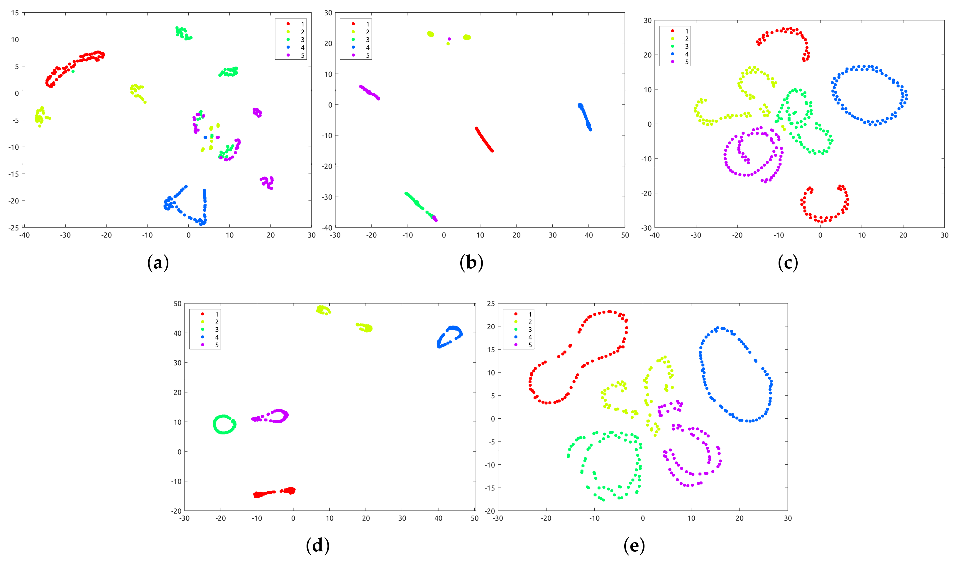
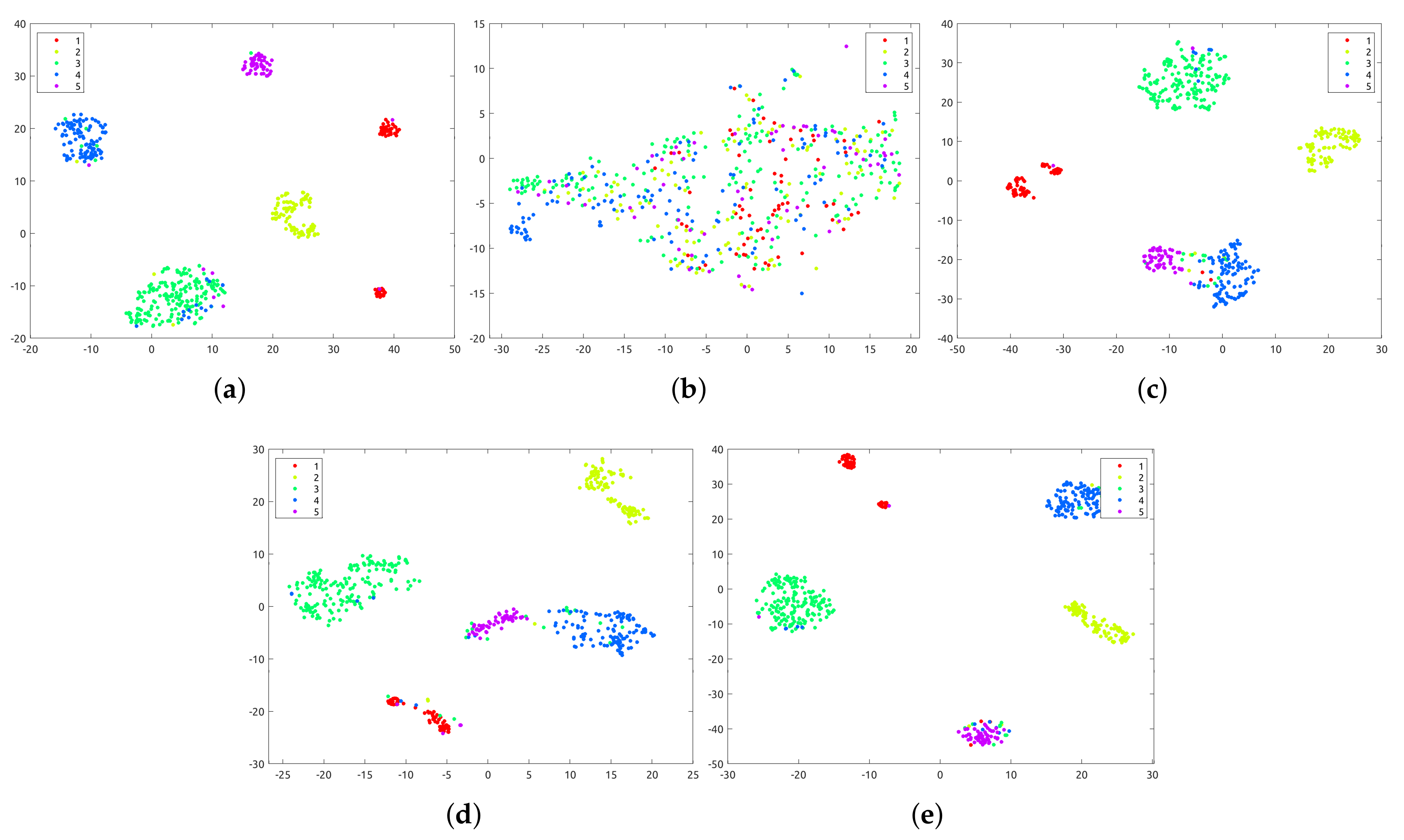
It is worth noting that MLAN, MCGC, GMC, and CGL are all multi-view clustering methods that involve the adaptive graph. From the results, we can say the proposed method that adopts the manifold topological structure has a superior performance, which further illustrates the effectiveness of adaptive manifold learning. Taking the datasets COIL-20 and BBCSport as examples, we carried out the t-SNE [36] to visualize the clustering results. As shown in Figure 2 and Figure 3, our model obviously achieves a much clearer clustering structure with better separability, and the gap between different clusters is evident, which further validates that our model can better uncover the intrinsic structure of the data. Considering that real-world data are usually sampled from a nonlinear low-dimensional manifold, our method is able to achieve a promising clustering performance in the general case.

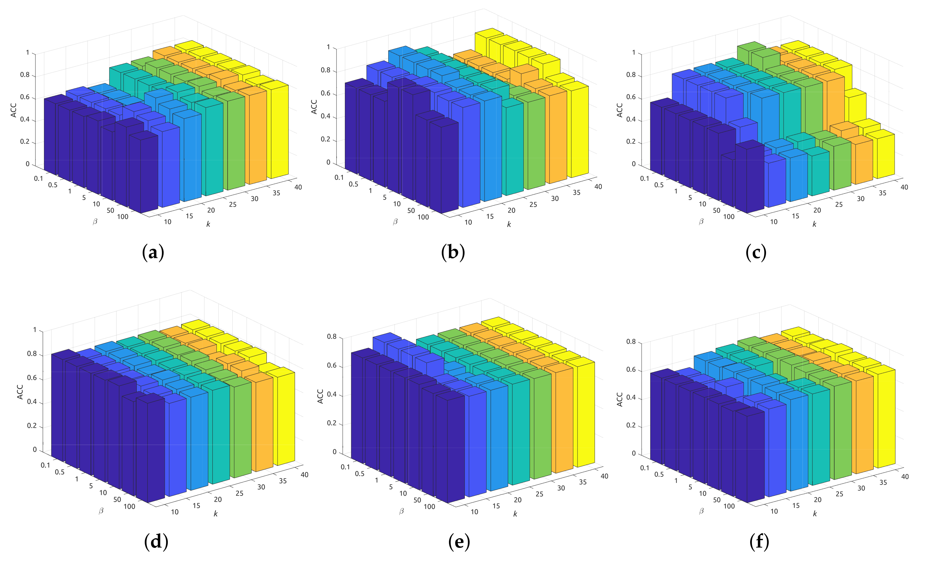
5.2. Sensitivity Analysis

We showcase the sensitivity of the proposed model with respect to different parameter settings. As described before, $\gamma$ is a self-adjusted parameter and can be tuned in a heuristic way. Thus, we only need to search the parameters $\alpha$ and $\beta$ properly. As mentioned in Equation (2), $\alpha$ can be determined according to the number of adaptive neighbors [10]. In this paper, we empirically search the adaptive neighbors k in the range [10,15,20,25,30,35,40] and $\beta$ in the range [0.1,0.5,1,5,10,50,100]. The clustering results of all datasets are plotted in Figure 4. It is obvious that our performance is relatively stable under a wide range of parameter settings, which pinpoints the robustness of our model. Generally speaking, we can expect a promising clustering performance when $\beta$ varies from 0.5 to 10, and k from 15 to 30, respectively.

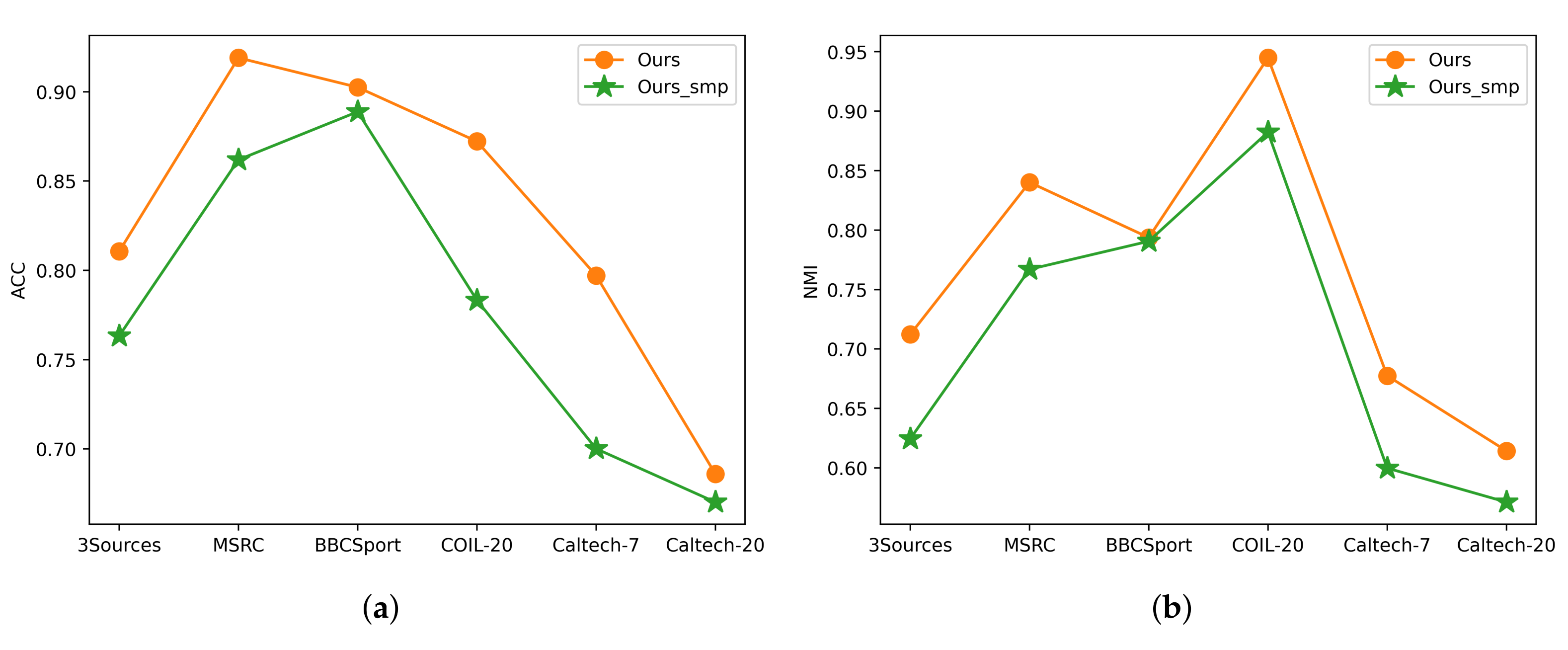
5.3. Ablation Study

In order to verify the importance of the auto-weight learning strategy in Equation (6), we tested a special case where all views are of the same importance to the clustering task, i.e., ${\mu }^{\left(v\right)}=\frac{1}{m}$, denoted as the simple version of our model. As shown in Figure 5, we report the clustering performance of two evaluation indexes (ACC and NMI) on six datasets, respectively. We can see that the experimental results of the auto-weight learning strategy (as described in Equation (6) are superior to those obtained by the simple average weighting strategy. Moreover, it can be seen that the overall improvement is remarkable, which obviously showcases the effectiveness of our auto-weight learning strategy.

5.4. Computational Performance

Given the computational complexity of our algorithm theoretical analyzed above, here, we empirically compare the computational speed of our method with other multi-view graph clustering approaches. The computational time of all algorithms on a machine with 2.60 GHz Intel Xeon Gold 6240 CPU and 256 GB RAM is shown in

Table 4. Comparison of computational time (seconds).

Dataset	SwMC	MLAN	AWP	WMSC	MCGC	CSMSC	GMC	COMSC	CGL	Ours
3Sources	0.51	0.11	0.08	0.16	0.50	0.19	0.22	27.29	0.34	0.66
MSRC	1.05	0.12	0.09	0.19	0.22	0.08	0.29	29.31	0.58	0.84
BBCSport	2.67	0.90	0.45	0.61	1.00	0.85	0.76	103.04	1.66	1.99
COIL-20	192.25	13.48	8.41	12.98	16.03	9.85	11.15	2015.47	26.08	10.94
Caltech-7	143.45	13.15	16.60	50.01	17.31	6.78	12.62	3493.87	54.16	19.89
Caltech-20	679.34	66.75	74.00	224.91	78.76	27.28	39.94	12484.65	201.20	75.11

. We see that COMSC and SwMC are the two timesaving-most algorithms, especially COMSC, which is slower than other methods by nearly two orders of magnitude. Generally speaking, our algorithm is faster than COMSC and SwMC and in line with other methods, which validates the efficiency of the proposed algorithm.

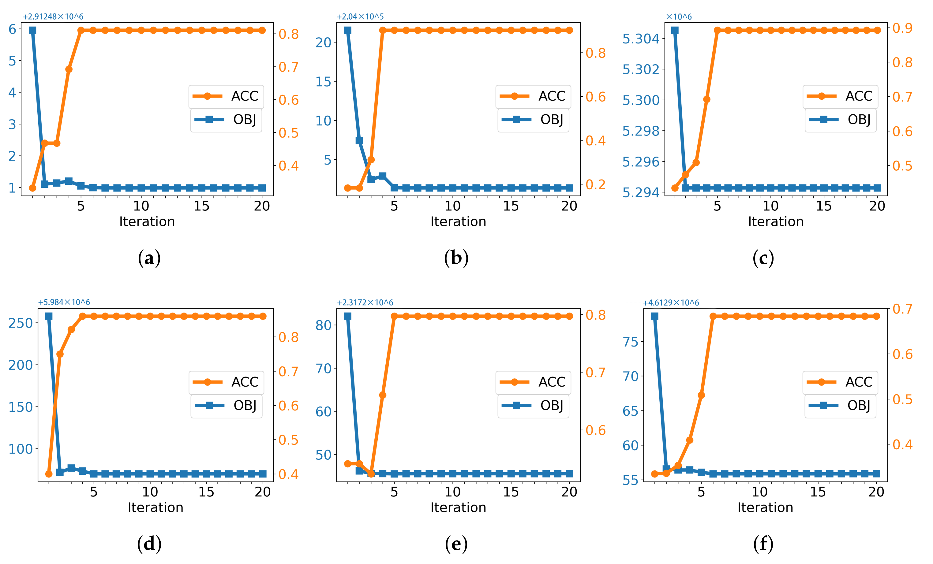
5.5. Convergence Study

The convergence property of our algorithm was theoretically analyzed previously. Here, we empirically validate the convergence speed of the proposed algorithm. The convergence curves along with the clustering results of our algorithm are shown in Figure 6, where the orange line represents the ACC of the proposed model, and the blue line denotes the value of the objective function. We can observe that the iterative updating algorithm converges very fast, which implies the efficiency of our algorithm.

6. Conclusions

In this paper, we explore the implied adaptive manifold for multi-view graph clustering. Our model seamlessly integrates multiple adaptive graphs into a consensus graph with the manifold topological structure considered. In addition, we manipulate the consensus graph with a useful rank constraint so that its connected components precisely correspond to distinct clusters. As a result, our model is able to directly achieve the discrete clustering result without any post-processing. An alternating iterative algorithm is introduced to solve the optimization problem. Experiments on several benchmark datasets illustrate the effectiveness of the proposed model, compared to the state-of-the-art algorithms in terms of four clustering evaluation metrics. In detail, the experimental results have shown that (1) our model achieved the best results in the majority of cases, (2) the proposed model is very stable across a wide range of parameter settings, and (3) the designed optimization algorithm is very efficient and converges fast. However, our model cannot deal with nonlinear data, which can be considered in future work. Furthermore, we are also interested in extending the proposed framework to other machine learning applications, such as medical data analysis and genetic data analysis.

References

1. Tang, C.; Zhu, X.; Liu, X.; Li, M.; Wang, P.; Zhang, C.; Wang, L. Learning a Joint Affinity Graph for Multiview Subspace Clustering. IEEE Trans. Multimed. 2019, 21, 1724–1736. [Google Scholar] [CrossRef]
2. Zhang, C.; Fu, H.; Hu, Q.; Cao, X.; Xie, Y.; Tao, D.; Xu, D. Generalized latent multi-view subspace clustering. IEEE Trans. Pattern Anal. Mach. Intell. 2018, 42, 86–99. [Google Scholar] [CrossRef] [PubMed]
3. Fan, S.; Wang, X.; Shi, C.; Lu, E.; Lin, K.; Wang, B. One2multi graph autoencoder for multi-view graph clustering. In Proceedings of the Web Conference 2020, Taipei, Taiwan, 20–24 April 2020; pp. 3070–3076. [Google Scholar]
4. Liu, J.; Liu, X.; Yang, Y.; Guo, X.; Kloft, M.; He, L. Multiview Subspace Clustering via Co-Training Robust Data Representation. IEEE Trans. Neural Networks Learn. Syst. 2021, 1–13. [Google Scholar] [CrossRef] [PubMed]
5. Jiang, R.; Yin, D.; Wang, Z.; Wang, Y.; Deng, J.; Liu, H.; Cai, Z.; Deng, J.; Song, X.; Shibasaki, R. DL-Traff: Survey and Benchmark of Deep Learning Models for Urban Traffic Prediction. In Proceedings of the 30th ACM International Conference on Information & Knowledge Management, Gold Coast, Australia, 1–5 November 2021; pp. 4515–4525. [Google Scholar]
6. Wu, H.; Lv, J.; Wang, J. Automatic Cataract Detection with Multi-Task Learning. In Proceedings of the International Joint Conference on Neural Networks, Shenzhen, China, 18–22 July 2021; pp. 1–8. [Google Scholar]
7. Nie, F.; Li, J.; Li, X. Self-weighted multiview clustering with multiple graphs. In Proceedings of the IJCAI, Melbourne, Australia, 19–25 August 2017; pp. 2564–2570. [Google Scholar]
8. Wang, X.; Fan, S.; Kuang, K.; Shi, C.; Liu, J.; Wang, B. Decorrelated clustering with data selection bias. In Proceedings of the IJCAI, Yokohama, Japan, 11–17 July 2020. [Google Scholar]
9. Kang, Z.; Shi, G.; Huang, S.; Chen, W.; Pu, X.; Zhou, J.T.; Xu, Z. Multi-graph fusion for multi-view spectral clustering. Knowl.-Based Syst. 2020, 189, 105102. [Google Scholar] [CrossRef] [Green Version]
10. Nie, F.; Wang, X.; Huang, H. Clustering and projected clustering with adaptive neighbors. In Proceedings of the KDD, New York, NY, USA, 24–27 August 2014; pp. 977–986. [Google Scholar]
11. Zhan, K.; Zhang, C.; Guan, J.; Wang, J. Graph learning for multiview clustering. IEEE Trans. Cybern. 2017, 48, 2887–2895. [Google Scholar] [CrossRef] [PubMed]
12. Nie, F.; Cai, G.; Li, X. Multi-View Clustering and Semi-Supervised Classification with Adaptive Neighbours. In Proceedings of the AAAI, San Francisco, CA, USA, 4–9 February 2017; pp. 2408–2414. [Google Scholar]
13. Zhuge, W.; Nie, F.; Hou, C.; Yi, D. Unsupervised single and multiple views feature extraction with structured graph. IEEE Trans. Knowl. Data Eng. 2017, 29, 2347–2359. [Google Scholar] [CrossRef]
14. Wang, H.; Yang, Y.; Liu, B. GMC: Graph-based Multi-view Clustering. IEEE Trans. Knowl. Data Eng. 2020, 32, 1116–1129. [Google Scholar] [CrossRef]
15. Zhan, K.; Nie, F.; Wang, J.; Yang, Y. Multiview consensus graph clustering. IEEE Trans. Image Process. 2018, 28, 1261–1270. [Google Scholar] [CrossRef] [PubMed]
16. Li, Z.; Tang, C.; Liu, X.; Zheng, X.; Yue, G.; Zhang, W.; Zhu, E. Consensus Graph Learning for Multi-view Clustering. IEEE Trans. Multimed. 2021, 24, 2461–2472. [Google Scholar] [CrossRef]
17. Wen, J.; Yan, K.; Zhang, Z.; Xu, Y.; Wang, J.; Fei, L.; Zhang, B. Adaptive graph completion based incomplete multi-view clustering. IEEE Trans. Multimed. 2020, 23, 2493–2504. [Google Scholar] [CrossRef]
18. Tkachenko, R.; Izonin, I. Model and principles for the implementation of neural-like structures based on geometric data transformations. In Proceedings of the International Conference on Computer Science, Engineering and Education Applications, Kiev, Ukraine, 18–20 January 2018; Springer: Berlin/Heidelberg, Germany, 2018; pp. 578–587. [Google Scholar]
19. Tkachenko, R. An Integral Software Solution of the SGTM Neural-Like Structures Implementation for Solving Different Data Mining Tasks. In Proceedings of the International Scientific Conference “Intellectual Systems of Decision Making and Problem of Computational Intelligence”, Zalizny Port, Ukraine, 24–28 May 2021; Springer: Berlin/Heidelberg, Germany, 2021; pp. 696–713. [Google Scholar]
20. Roweis, S.T.; Saul, L.K. Nonlinear dimensionality reduction by locally linear embedding. Science 2000, 290, 2323–2326. [Google Scholar] [CrossRef] [PubMed] [Green Version]
21. Zhang, Z.; Wang, J.; Zha, H. Adaptive manifold learning. IEEE Trans. Pattern Anal. Mach. Intell. 2011, 34, 253–265. [Google Scholar] [CrossRef] [PubMed] [Green Version]
22. Minh, H.Q.; Bazzani, L.; Murino, V. A unifying framework in vector-valued reproducing kernel hilbert spaces for manifold regularization and co-regularized multi-view learning. J. Mach. Learn. Res. 2016, 17, 1–72. [Google Scholar]
23. Wang, Q.; Chen, M.; Li, X. Quantifying and detecting collective motion by manifold learning. In Proceedings of the AAAI, San Francisco, CA, USA, 4–9 February 2017; pp. 4292–4298. [Google Scholar]
24. Huang, S.; Tsang, I.; Xu, Z.; Lv, J.C. Measuring Diversity in Graph Learning: A Unified Framework for Structured Multi-view Clustering. IEEE Trans. Knowl. Data Eng. 2021, 1–15. [Google Scholar] [CrossRef]
25. Nie, F.; Li, J.; Li, X. Parameter-free auto-weighted multiple graph learning: A framework for multiview clustering and semi-supervised classification. In Proceedings of the IJCAI, New York, NY, USA, 9–15 July 2016; pp. 1881–1887. [Google Scholar]
26. Huang, S.; Kang, Z.; Tsang, I.W.; Xu, Z. Auto-weighted multi-view clustering via kernelized graph learning. Pattern Recognit. 2019, 88, 174–184. [Google Scholar] [CrossRef]
27. Fan, K. On a theorem of Weyl concerning eigenvalues of linear transformations I. Proc. Natl. Acad. Sci. USA 1949, 35, 652–655. [Google Scholar] [CrossRef] [PubMed] [Green Version]
28. Huang, J.; Nie, F.; Huang, H. A new simplex sparse learning model to measure data similarity for clustering. In Proceedings of the IJCAI, Buenos Aires, Argentina, 25–31 July 2015; pp. 3569–3575. [Google Scholar]
29. Bertsekas, D.P. Nonlinear programming. J. Oper. Res. Soc. 1997, 48, 334. [Google Scholar] [CrossRef]
30. Bazaraa, M.S.; Sherali, H.D.; Shetty, C.M. Nonlinear Programming: Theory and Algorithms; John Wiley & Sons: Hoboken, NJ, USA, 2013. [Google Scholar]
31. Nie, F.; Huang, H.; Cai, X.; Ding, C.H. Efficient and robust feature selection via joint 2,1-norms minimization. In Proceedings of the Advances in Neural Information Processing Systems, Virtual, 6–12 December 2010; pp. 1813–1821. [Google Scholar]
32. Nie, F.; Tian, L.; Li, X. Multiview clustering via adaptively weighted procrustes. In Proceedings of the KDD, London, UK, 19–23 August 2018; pp. 2022–2030. [Google Scholar]
33. Zong, L.; Zhang, X.; Liu, X.; Yu, H. Weighted multi-view spectral clustering based on spectral perturbation. In Proceedings of the AAAI, New Orleans, LA, USA, 2–7 February 2018; pp. 4621–4628. [Google Scholar]
34. Luo, S.; Zhang, C.; Zhang, W.; Cao, X. Consistent and Specific Multi-View Subspace Clustering. In Proceedings of the AAAI, New Orleans, LA, USA, 2–7 February 2018; Volume 32. [Google Scholar]
35. Zhang, P.; Liu, X.; Xiong, J.; Zhou, S.; Zhao, W.; Zhu, E.; Cai, Z. Consensus One-step Multi-view Subspace Clustering. IEEE Trans. Knowl. Data Eng. 2020. [Google Scholar] [CrossRef]
36. Van der Maaten, L.; Hinton, G. Visualizing data using t-SNE. J. Mach. Learn. Res. 2008, 9, 2579–2605. [Google Scholar]
Figure 1. Illustration of topological relevance. The red data sample and the green data sample show a low similarity on spatial velocity, but they maintain high topological relevance to each other.
Mathematics 10 01821 g001
Figure 2. Visualization of the clustering results of the first 5 classes of COIL-20 with t-SNE. (a) MLAN. (b) MCGC. (c) GMC. (d) CGL. (e) Ours.
Mathematics 10 01821 g002
Figure 3. Visualization of the clustering results of the first 5 classes of BBCSport with t-SNE. (a) MLAN. (b) MCGC. (c) GMC. (d) CGL. (e) Ours.
Mathematics 10 01821 g003
Figure 4. Accuracy (ACC) with respect to β and the number of neighbors (k). (a) 3Sources. (b) MSRC. (c) BBCSport. (d) COIL-20. (e) Caltech-7. (f) Caltech-20.
Mathematics 10 01821 g004
Figure 5. Auto-weight learning strategy (adopted in Our original model) vs. average weighting strategy (denoted by Ours_smp). (a) ACC. (b) NMI.
Mathematics 10 01821 g005
Figure 6. Convergence analysis of the proposed method, where OBJ denotes the objective value. (a) 3Sources. (b) MSRC. (c) BBCSport. (d) COIL-20. (e) Caltech-7. (f) Caltech-20.
Mathematics 10 01821 g006