An Efficient Computational Technique for the Electromagnetic Scattering by Prolate Spheroids

Abstract

In this paper we present an efficient Matlab computation of a 3-D electromagnetic scattering problem, in which a plane wave impinges with a generic inclination onto a conducting ellipsoid of revolution. This solid is obtained by the rotation of an ellipse around one of its axes, which is also known as a spheroid. We have developed a fast and ad hoc code to solve the electromagnetic scattering problem, using spheroidal vector wave functions, which are special functions used to describe physical problems in which a prolate or oblate spheroidal reference system is considered. Numerical results are presented, both for TE and TM polarization of the incident wave, and are validated by a comparison with results obtained by a commercial electromagnetic simulator.

1. Introduction

In electromagnetic scattering problems it is often useful to refer to cases where scatterers are two-dimensional objects immersed in non-homogeneous scenarios, as in ground-penetrating radar, through-the-wall radar or wireless power transfer system applications with wearable or implantable devices [1,2,3,4,5,6,7,8]. For other specific applications, ranging from finding people in dangerous situations, such as after earthquakes, or in biological applications, it could be more interesting to model three-dimensional objects by means of spherical or spheroidal geometries.

To this aim, the use of spheroidal wave functions is appropriate. The latter, introduced by Hansen in 1935, are special functions widely used in mathematical physics where a prolate or oblate spheroidal reference system is used [9,10,11,12,13,14,15,16], and also have important applications in electromagnetic scattering problems. Spheroidal reference systems are used in applications which include, for example, the modelling of raindrops, in the calculation of rain attenuation of microwave signals in line-of-sight, and satellite telecommunication systems or the modelling of a human head in the calculation of the electromagnetic interaction between a head and a mobile phone [17,18].

Several analytical solutions involving spheroidal functions have been obtained over the years, [19,20,21,22,23,24,25,26] such as the field and current distribution analysis of a prolate spheroidal dipole antenna embedded in a larger dielectric confocal prolate spheroid with finite conductivity, carried out by Jen [27], and the exact solution for scattering from conducting prolate spheroids by an axially incident plane wave, proposed by Schultz [28]. Reitlinger provided the general solution for arbitrary incidence and arbitrary polarization but no numerical results were presented [29]. This approach presents two main disadvantages: one concerns a process of matrix inversion, which must be repeated each time the angle of incidence of the source is changed, and the second is that the matrix from which the coefficients of the scattered field are obtained cannot be used to determine the coefficients of the other polarization. The problem of the matrix inversion was removed by Sinha and MacPhie [30], who presented a solution involving matrices depending only on the scatterer.

In this contribution, we referred to the theory developed in [30] and proposed an efficient numerical implementation for both TE and TM modes. This implementation made use of a library of functions already available where the authors were not aware that they had ever been used for electromagnetic scattering problems. Truncation criteria previously proposed by other authors have been revisited. Comparisons with a commercial numerical electromagnetic solver, performed for both polarizations, several incident wave directions, and different scatterer shapes, have shown a good agreement. The paper is organized as follows. In Section 2 we summarize the analytical approach, in Section 3 we discuss the numerical implementation and present the results through a comparison with a commercial electromagnetic simulator. In Section 4 we draw the conclusions.

2. Theoretical Analysis

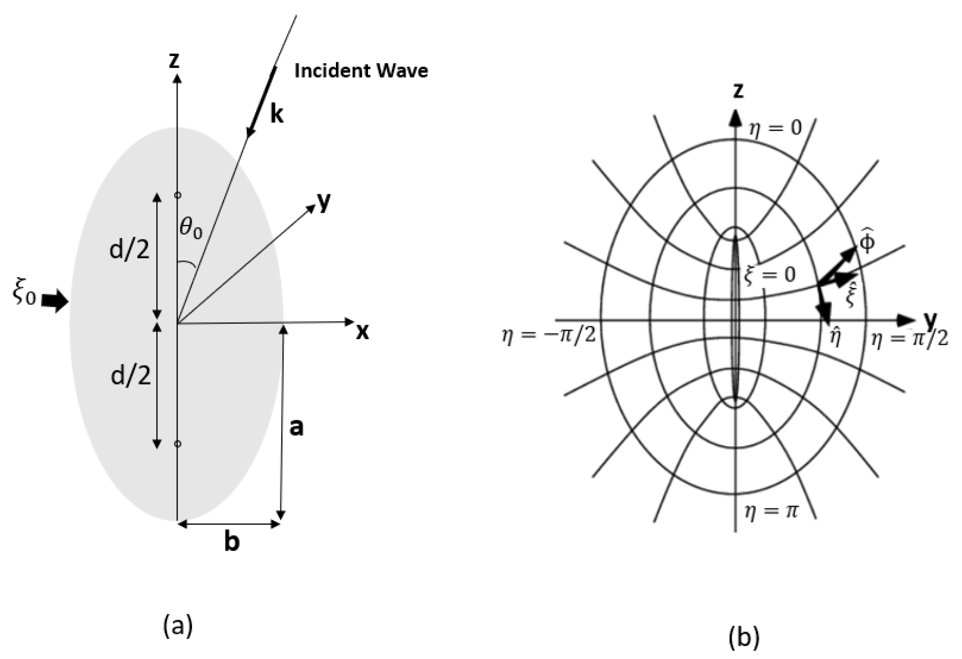
We are interested in studying the electromagnetic scattering of a plane, linearly polarized, monochromatic wave (with wavelength $\lambda$) from a perfectly conducting prolate spheroid. The spheroid was immersed in a homogeneous, isotropic, non-conductive, and non-magnetic medium. The geometry of the scattering problem is illustrated in Figure 1a, where the prolate spheroidal coordinates are related to the Cartesian coordinates by the following relations [20] (see Figure 1b):

$$\left\{\begin{array}{c}{\displaystyle x=\frac{d}{2}\sqrt{(1-{\eta }^2)({\xi }^2-1)}cos\varphi }\\ \\ {\displaystyle y=\frac{d}{2}\sqrt{(1-{\eta }^2)({\xi }^2-1)}sin\varphi }\\ \\ {\displaystyle z=\frac{d}{2}\eta \xi }\end{array}\right.$$

where d is the interfocal distance and $-1\le \eta \le 1,1\le \xi <\infty ,0\le \varphi \le 2\pi$.

The surface at $\xi ={\xi }_0=constant>1$ forms an elongated ellipsoid of revolution with major axis of length $d\xi$ and minor axis of length $d\sqrt{{\xi }^2-1}$. The value of ${\xi }_0$ is related to the major and minor axes of the ellipse (a and b, respectively) by the following relation:

$${\displaystyle {\xi }_0=\frac{a}{\sqrt{a^2-b^2}}=\frac{a/b}{\sqrt{{(a/b)}^2-1}}.}$$

We assume, without loss of generality, that the direction of propagation of the incident wave is in the $xz$-plane, and forms the angle ${\theta }_0$ with the z-axis. The plane-wave expressions for TE polarization (electric field normal to the $xz$-plane) and for TM polarization (electric field lying in the $xz$-plane), at a point of coordinates $\mathbf{r}$, are

$${\mathbf{E}}_{\mathrm{i}}^{\mathrm{TE}}\left(\mathbf{r}\right)={\mathrm{E}}_{\mathrm{i}0}^{\mathrm{TE}}{e}^{-j\mathbf{k}·\mathbf{r}}\widehat{y},$$

(1)

$${\mathbf{E}}_{\mathrm{i}}^{\mathrm{TM}}\left(\mathbf{r}\right)={\mathrm{E}}_{\mathrm{i}0}^{\mathrm{TM}}{e}^{-j\mathbf{k}·\mathbf{r}}(-\widehat{x}cos{\theta }_0+\widehat{z}sin{\theta }_0),$$

(2)

where ${\mathrm{E}}_{\mathrm{i}0}^{\mathrm{TE}}$ and ${\mathrm{E}}_{\mathrm{i}0}^{\mathrm{TM}}$ are the field amplitudes, $\mathbf{k}=-k(\widehat{x}sin{\theta }_0+\widehat{z}cos{\theta }_0$) is the propagation vector, with $k=2\pi /\lambda$. The temporal dependence, of the form $exp\left(j\omega t\right)$, is omitted for brevity.

Considering prolate spheroidal coordinates, the separation of scalar variables results in three independent functions: the radial spheroidal function $R_{mn}^{\left(i\right)}$, the angular spheroidal function $S_{mn}$ [20], and the sine and cosine functions. The expansion of a plane wave in terms of prolate spheroidal wave functions, given in [20], has the following expression:

$${\displaystyle e^{-j\mathbf{k}·\mathbf{r}}=2\sum _{m=0}^{\infty }\sum _{m=n}^{\infty }\frac{{ϵ}_m{j}^n}{N_{mn}\left(c\right)}{S}_{mn}(c,cos{\theta }_0)S_{mn}(c,\eta )R_{mn}^{\left(1\right)}(c,\xi )cos\left(m\varphi \right)}$$

(3)

where

$${\displaystyle c=\frac{1}{2}kd,}$$

${ϵ}_m$ is the Neumann number (${ϵ}_m=1$ for $m=0$ and ${ϵ}_m=2$ for $m>0$), and $N_{mn}\left(c\right)$ is the normalization factor of the angular function of the first kind.

It is possible to rewrite Equations (1) and (2) in terms of vector wave functions [20] as follows:

$${\mathbf{E}}_{\mathrm{i}}^{\mathrm{TE}}=\frac{{\mathrm{E}}_{\mathrm{i}0}^{\mathrm{TE}}}{kcos{\theta }_0}\sum _{n=m}^{\infty }\sum _{m=0}^{\infty }{A}_{mn}(c,{\theta }_0){\mathbf{M}}_{emn}^{x\left(1\right)}(c;\eta ,\xi ,\varphi ),$$

(4)

$${\mathbf{E}}_{\mathrm{i}}^{\mathrm{TM}}=\frac{{\mathrm{E}}_{\mathrm{i}0}^{\mathrm{TM}}}{k}\sum _{n=m}^{\infty }\sum _{m=0}^{\infty }{A}_{mn}(c,{\theta }_0){\mathbf{M}}_{emn}^{y\left(1\right)}(c;\eta ,\xi ,\varphi ),$$

(5)

where

$$A_{mn}(c,{\theta }_0)=\frac{2{ϵ}_m{j}^{n-1}}{N_{mn}}{S}_{mn}(c,cos{\theta }_0)$$

and the $\mathbf{M}$ vectors are the vector spheroidal wave functions, given in [20].

Taking into account that the scattered fields must satisfy the radiation condition at infinity, their expressions for TE and TM incident fields can be written as follows [30]:

$${\mathbf{E}}_{\mathrm{s}}^{\mathrm{TE}}=\sum _{m=0}^{\infty }\sum _{n=m}^{\infty }({\alpha }_{mn}{\mathbf{M}}_{em+1,n}^{+\left(4\right)}+{\gamma }_{mn}{\mathbf{M}}_{emn}^{z\left(4\right)})$$

(6)

and

$${\mathbf{E}}_{\mathrm{s}}^{\mathrm{TM}}=\sum _{m=0}^{\infty }\sum _{n=m}^{\infty }({\beta }_{mn}{\mathbf{M}}_{om+1,n}^{+\left(4\right)}+{\rho }_{m+1,n+1}{\mathbf{M}}_{om+1,n+1}^{z\left(4\right)})+\sum _{n=1}^{\infty }{\beta }_{1n}^{-}{\mathbf{M}}_{o1n}^{-\left(4\right)}$$

(7)

respectively, where ${\alpha }_{mn}$, ${\beta }_{mn}$, ${\gamma }_{mn}$, ${\rho }_{m+1,n+1}$, ${\beta }_{1n}^{-}$ are expansion coefficients.

Considering a perfectly conducting prolate spheroid, the boundary conditions to be imposed at the surface of the spheroid $\xi ={\xi }_0$ are as follows:

$$\left\{\begin{array}{c}{E}_{\mathrm{i}\eta }+E_{\mathrm{s}\eta }=0,\\ \\ E_{\mathrm{i}\varphi }+E_{\mathrm{s}\varphi }=0\end{array}\right.$$

(8)

where the subscripts $\eta$ and $\varphi$ denote, respectively, the $\eta$- and $\varphi$-components of the fields.

Let us first consider the TE polarization case. Inserting the expressions of the incident field (4) and the scattered field (6) into (8), we obtain the following, after some algebra:

$${(cos{\theta }_0)}^{-1}{\mathbf{Q}}_m^E{\mathbf{A}}_m=\left({\mathbf{R}}_m^E\right){\mathbf{S}}_m^E,m=0,1,2,\dots ,$$

and

$${(cos{\theta }_0)}^{-1}\left({\mathbf{Q}}_{+}^E\right){\mathbf{A}}_{+}=\left({\mathbf{R}}_{+}^E\right){\mathbf{S}}_{+}^E$$

(9)

where the expressions of ${\mathbf{Q}}_{+}^E$, ${\mathbf{A}}_{+}$, ${\mathbf{R}}_{+}^E$, ${\mathbf{S}}_{+}^E$, ${\mathbf{Q}}_m^E$, ${\mathbf{Q}}_{mm}^E$ and ${\mathbf{Q}}_{m,m+2}^E$ are given in [30]. The scattering column vector ${\mathbf{S}}^E$ can be obtained from the incident column vector ${\mathbf{I}}^E$ via the following transformation:

$${\mathbf{S}}^E=\left({\mathbf{G}}^E\right){\mathbf{I}}^E,$$

where

$$\left({\mathbf{G}}^E\right)=\left(\begin{array}{cccc}{\left({\mathbf{R}}_{+}^E\right)}^{-1}\left({\mathbf{Q}}_{+}^E\right)& \mathbf{0}& \mathbf{0}& \cdots \\ \mathbf{0}& {\left({\mathbf{R}}_0^E\right)}^{-1}\left({\mathbf{Q}}_0^E\right)& \mathbf{0}& \cdots \\ \mathbf{0}& \mathbf{0}& {\left({\mathbf{R}}_1^E\right)}^{-1}\left({\mathbf{Q}}_1^E\right)& \cdots \\ ⋮& ⋮& ⋮& ⋮\end{array}\right).$$

We consider now TM polarization of the incident wave. Inserting Equations (5) and (7) into (8), and using the orthogonality of the trigonometric functions and the spheroidal angular functions, we get

$$\left({\mathbf{Q}}^M\right){\mathbf{A}}_m=\left({\mathbf{R}}_m^E\right){\mathbf{S}}_m^M,m=0,1,2\dots ,$$

and

$$\left({\mathbf{Q}}_{+}^M\right){\mathbf{A}}_{+}=\left({\mathbf{R}}_{+}^M\right){\mathbf{S}}_{+}^M,$$

where $\left[Q_m^M\right]$, ${\mathbf{R}}_m^E$, ${\mathbf{A}}_m$, ${\mathbf{A}}_{+}$ are defined in [30]. We obtain, in the same way, the following matrix transformation:

$${\mathbf{S}}^M=\left({\mathbf{G}}^M\right){\mathbf{I}}^M,$$

3. Numerical Results and Discussion

The analytical method presented in Section 2 has been numerically implemented in Matlab. The $\mathtt{spheroidal}$ library was used to calculate the spheroidal wave functions [31], allowing the use of arbitrary precision arithmetic and the adaptive choosing of the number of expansion coefficients.

The arbitrary precision arithmetic was achieved by the GNU MPFR library [32]. It provided good accuracy in many of the computations, especially for high wave numbers and modes. All the examples in this paper were obtained using a precision of 500 bits. A preliminary step in the numerical evaluation of the spheroidal functions consisted of computing and storing the characteristic values and the expansion coefficients in order to speed-up the computations of the subsequent functions.

In the numerical evaluations, a truncation was introduced on the matrices and series described in the previous section. In accordance with [30] we used the following truncation rules:

$$m_t=⌊ka+4⌋,$$

where $⌊·⌋$ denotes the floor function, and all summations in Equations (3)–(7) are for $m=0,\dots ,(m_t-1)$ and $n=m,\dots ,(m_t-1)$.

3.1. TE Polarization

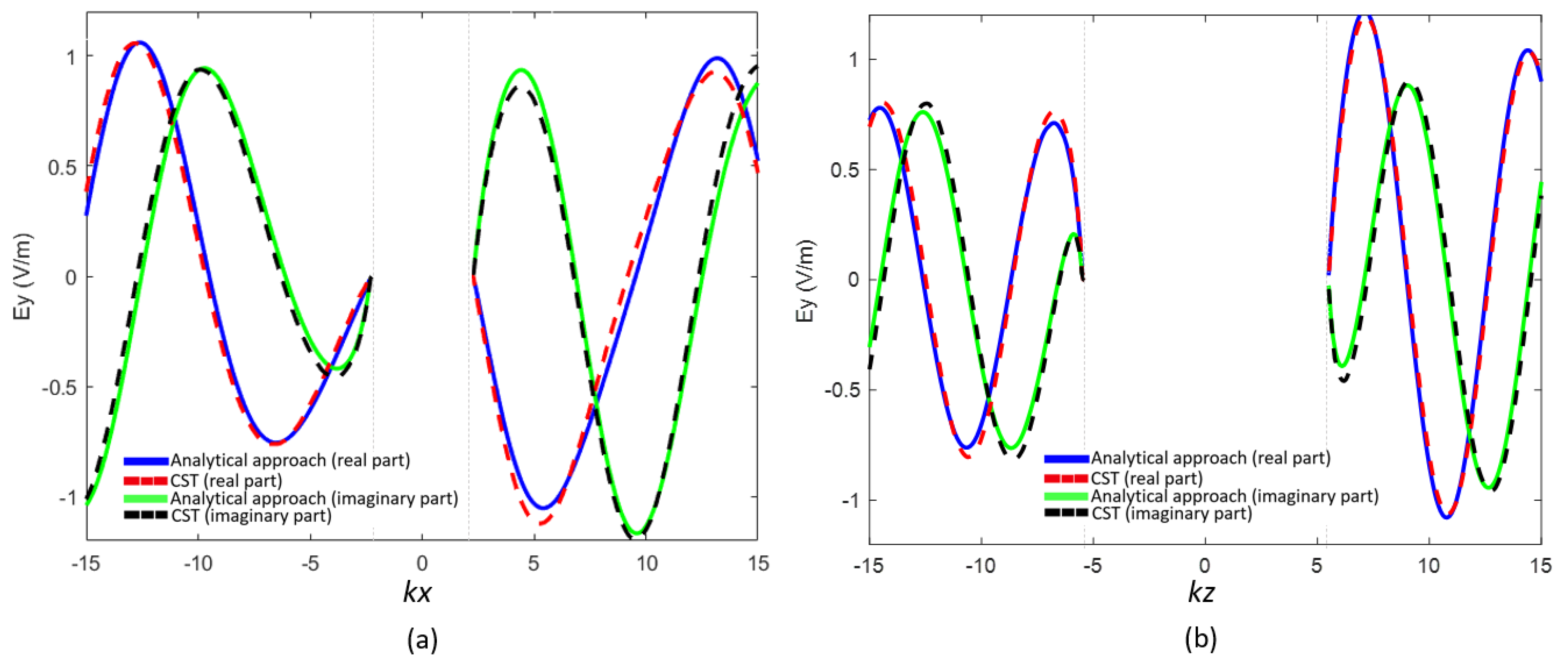
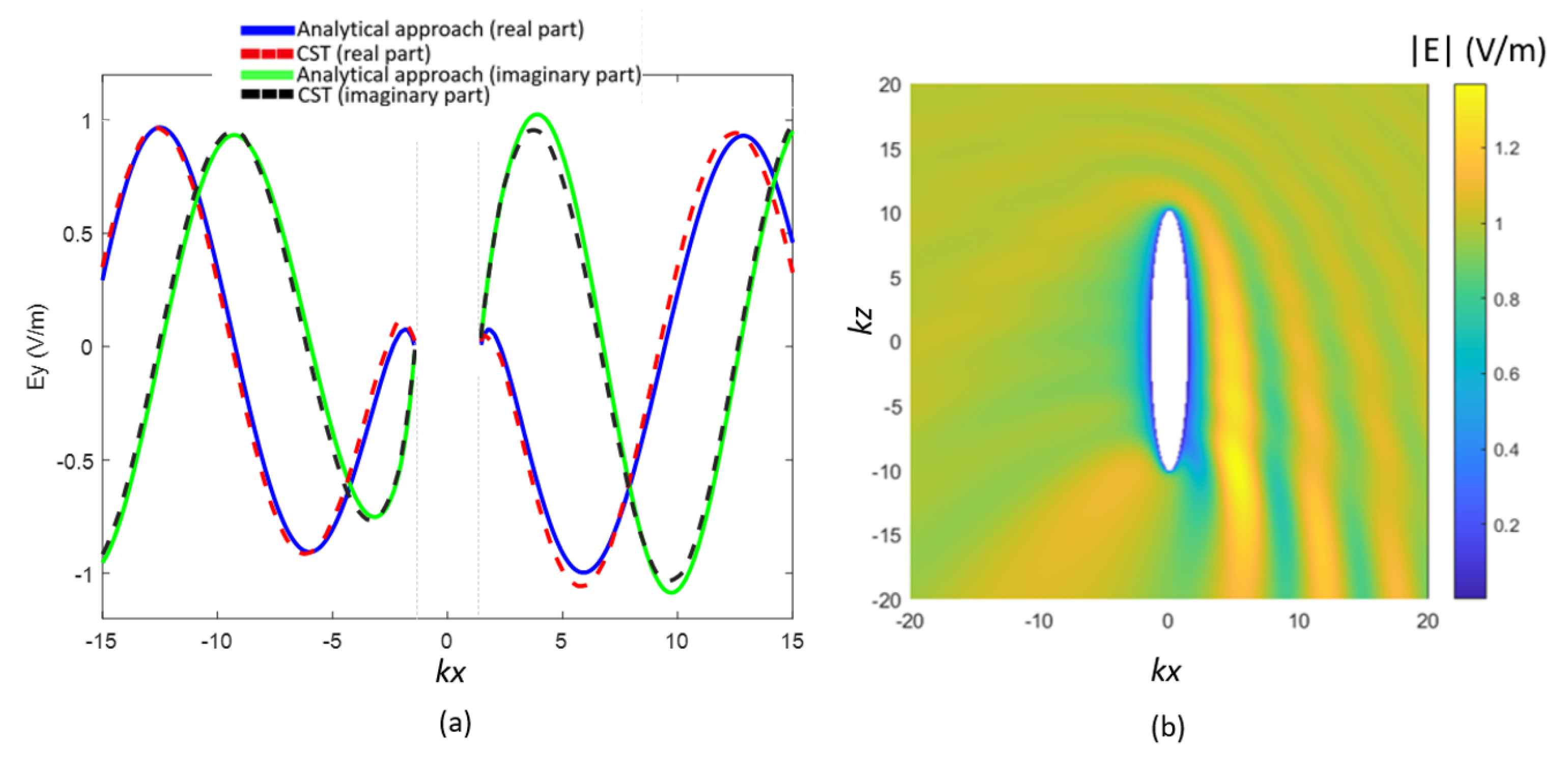
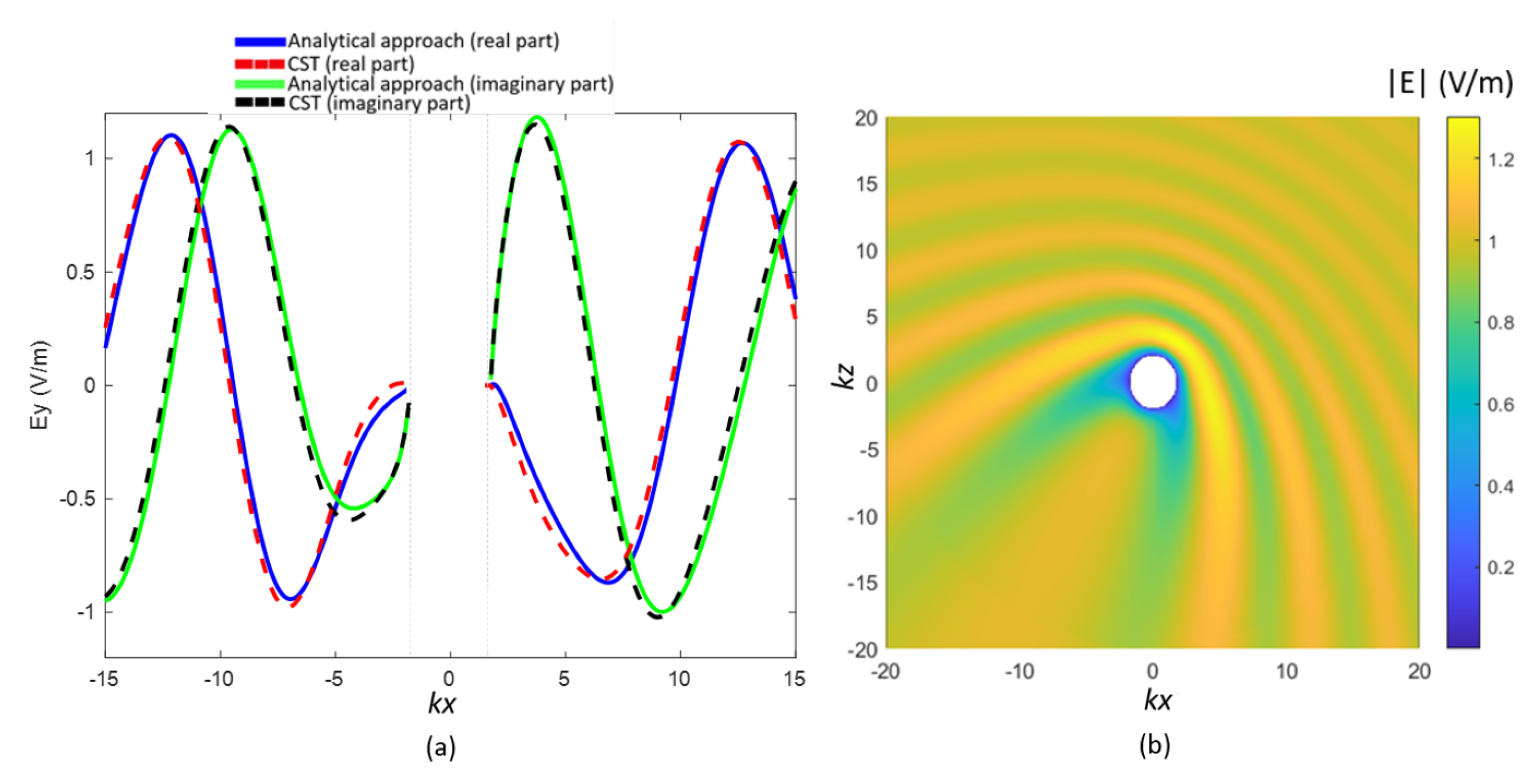
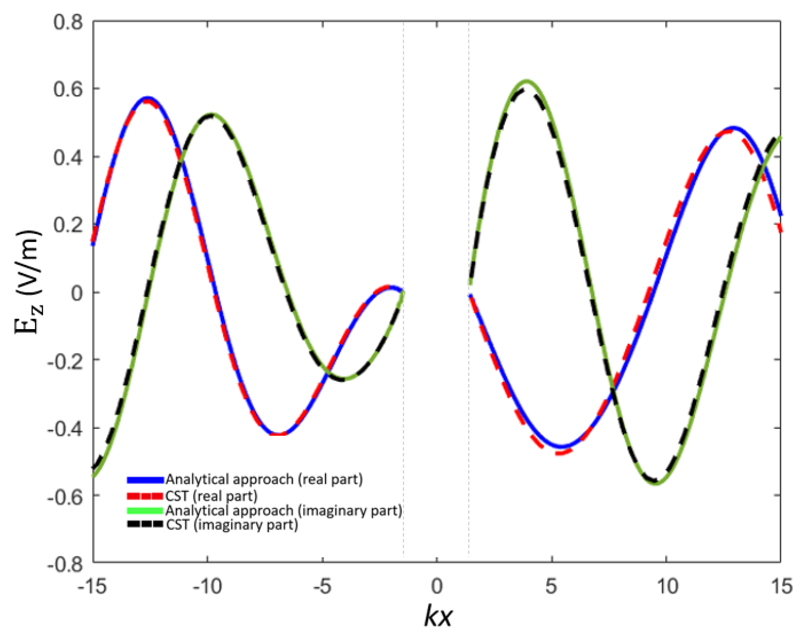
We first consider the case of TE polarization where the incident wave impinges onto the prolate spheroid with the incidence angle ${\theta }_0={30}^{\circ }$. In such a case the electric field of the incident wave is perpendicular to the incidence plane. The geometric parameters of the scatterer were ${\xi }_0=1.1$ and $kd=10$ (corresponding to $ka=5.5$, $kb=2.2913$, $c=5$, and $m_t=9$). The validation of our Matlab code is shown in Figure 2 through a comparison with the results obtained by modelling the spheroid in CST Microwave Studio. In particular, Figure 2a shows the real and imaginary parts of the electric field $E_y$ along the x-axis and Figure 2b shows those along the z-axis. In all the simulations performed in CST Microwave Studio with the time domain solver, the computation domain was meshed with hexahedral cells with sizes between $0.16/k$ and $0.33/k$. It could be seen that the agreement was excellent.

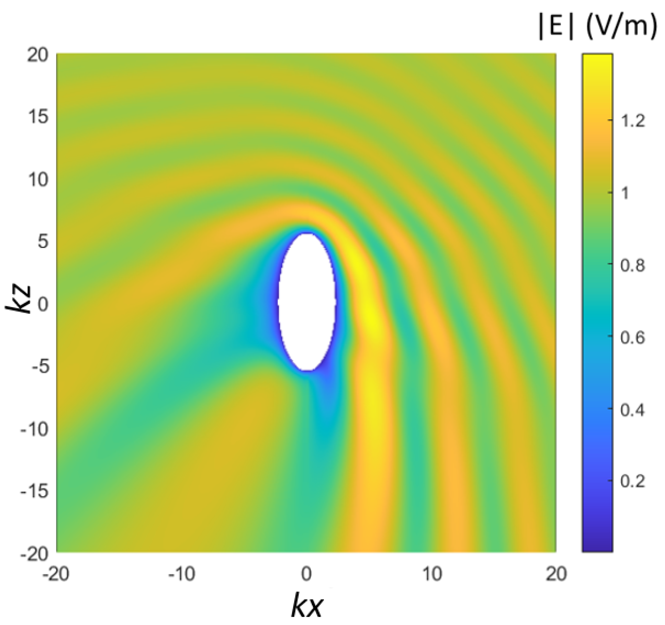
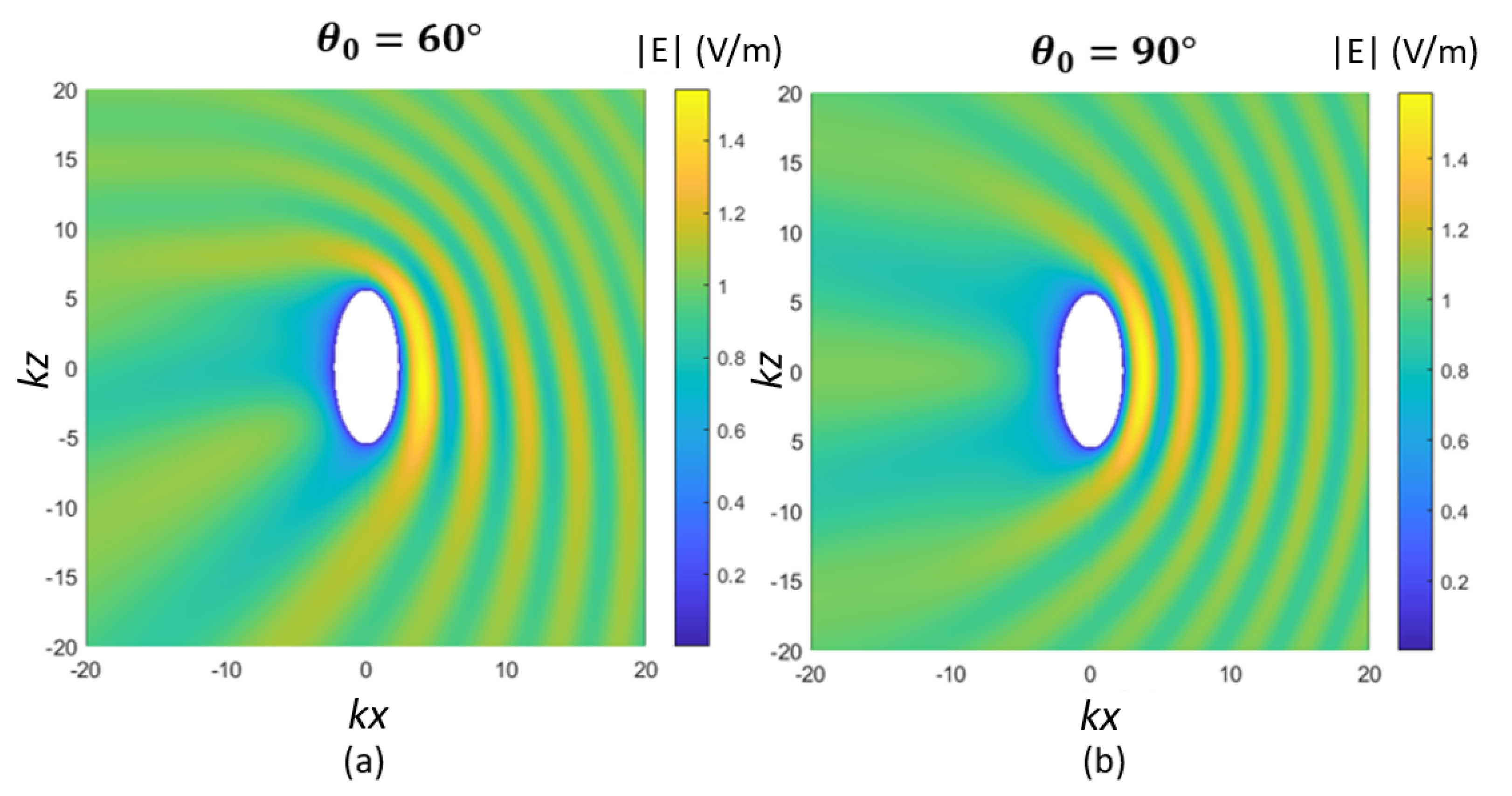
The magnitude of the electric field across the $xz$-plane is presented in Figure 3 for the same geometrical parameters considered in Figure 2. In Figure 4 the results obtained for different angles of incidence (${\theta }_0={60}^{\circ }$ and ${\theta }_0={90}^{\circ }$) are presented. The case of orthogonal incidence (${\theta }_0={90}^{\circ }$) was a special case, where the scattering column vector in Equation (9) is given by:

$${\mathbf{S}}^E=\left({\mathbf{G}}^E\right){\mathbf{I}}^E,$$

and ${\mathbf{I}}^E$ is obtained from $\mathbf{A}$ by replacing $A_{mn}$ by the following coefficients:

$$B_{mn}=0,\mathrm{with}(n-m)\mathrm{even}$$

$$B_{mn}=2\frac{{ϵ}_m{j}^{n-1}}{N_{mn}}\sum _{k=0}^{\infty }{c}_{2k}^{mn}=2\frac{{ϵ}_m{j}^{n-1}{(-1)}^{(n-m-1)/2}(n+m+1)!}{2^n\left(\frac{n-m-1}{2}\right)!\left(\frac{n+m+1}{2}\right)!},\mathrm{with}(n-m)\mathrm{odd}.$$

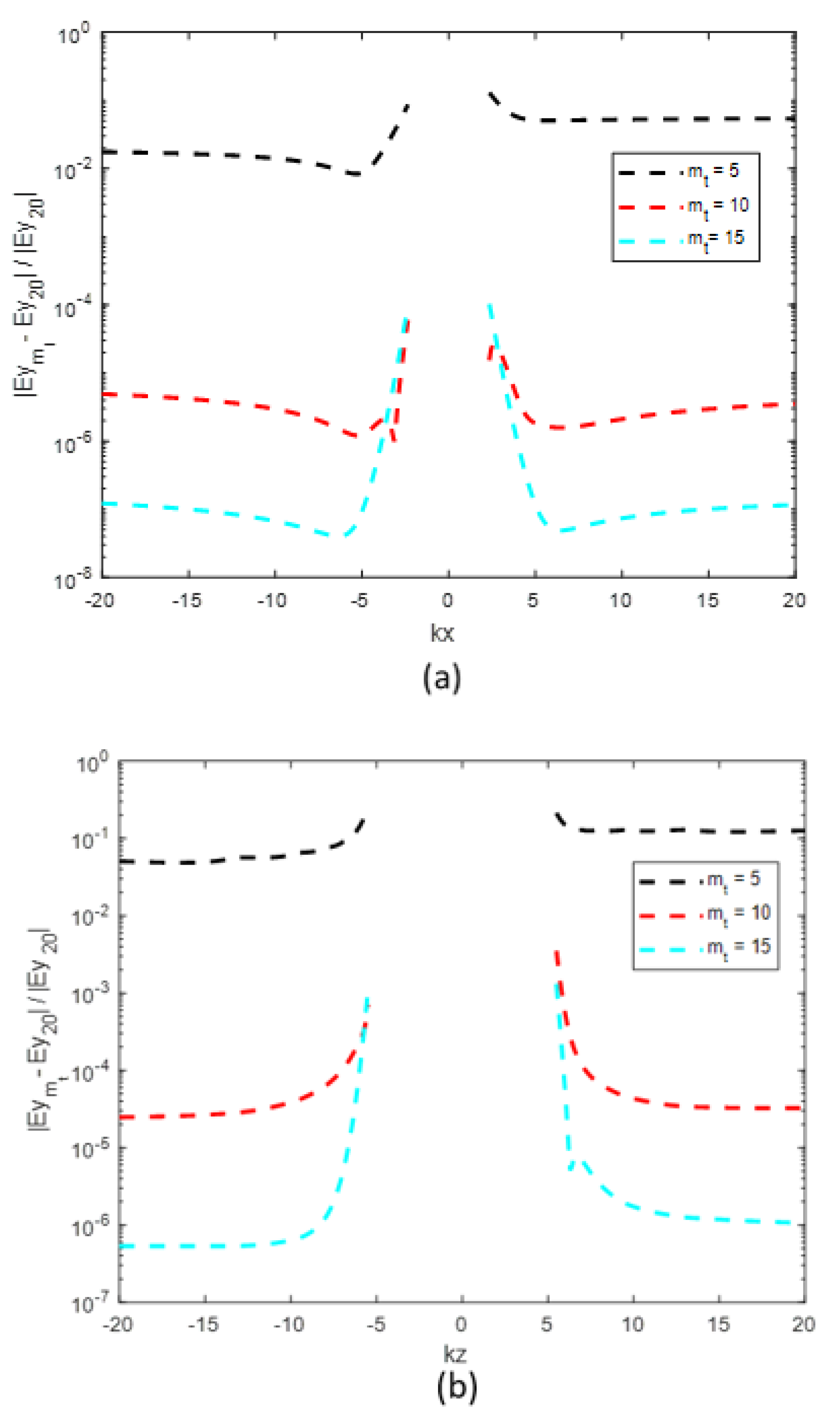
In order to validate the adopted truncation rule ($m_t=10$, in this case), we considered several cases with different truncation orders. In particular, we compared the results obtained with $m_t=5$, $m_t=10$ and $m_t=15$, to those obtained with a large value of $m_t$, for which the convergence of the method was taken for granted ($m_t=20$). As shown in Figure 5, the relative difference of the electric field magnitude was alway less than ${10}^{-4}$ when $m_t=10$.

Figure 6 shows the amplitudes of the terms of the $\mathbf{G}$ matrix for the geometrical parameters considered in Figure 5, with $m_t=9$. The matrix was composed of $99\times 99$ terms.

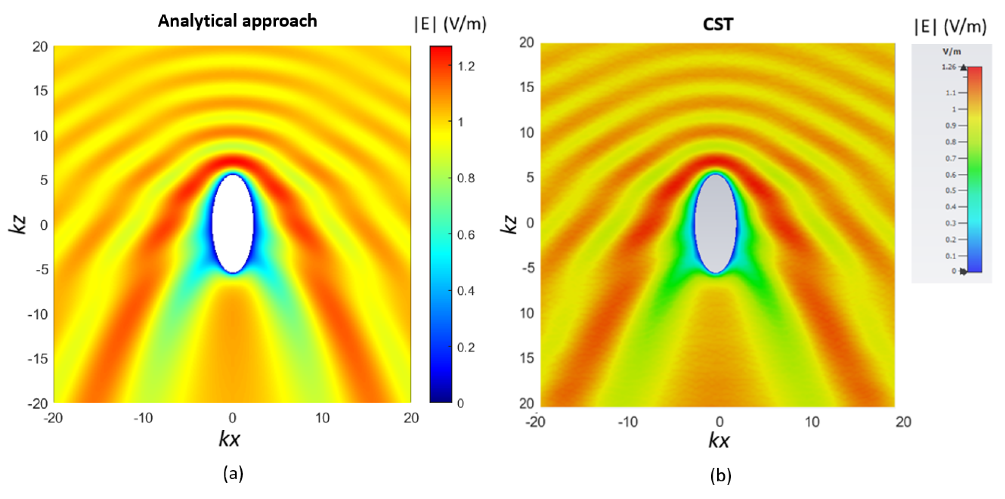
The case of axial incidence (${\theta }_0=0^{\circ }$) was also considered. In this case, the solution was greatly simplified by virtue of the symmetry. Figure 7 shows the magnitude of the E-field across the $xz$-plane for the incidence angle ${\theta }_0=0^{\circ }$, and the comparison between the results obtained from the analytical approach implemented in Matlab (a) and CST (b).

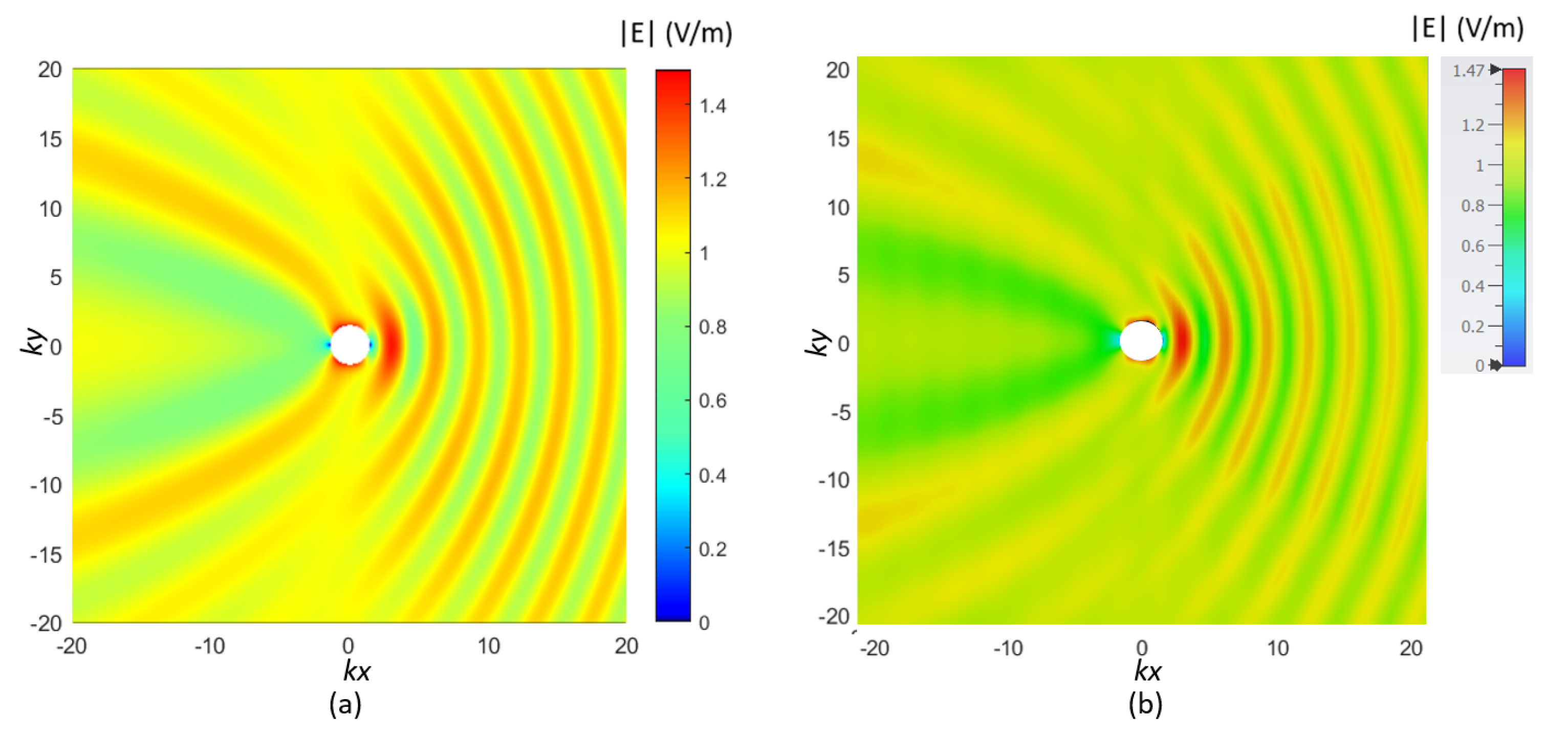
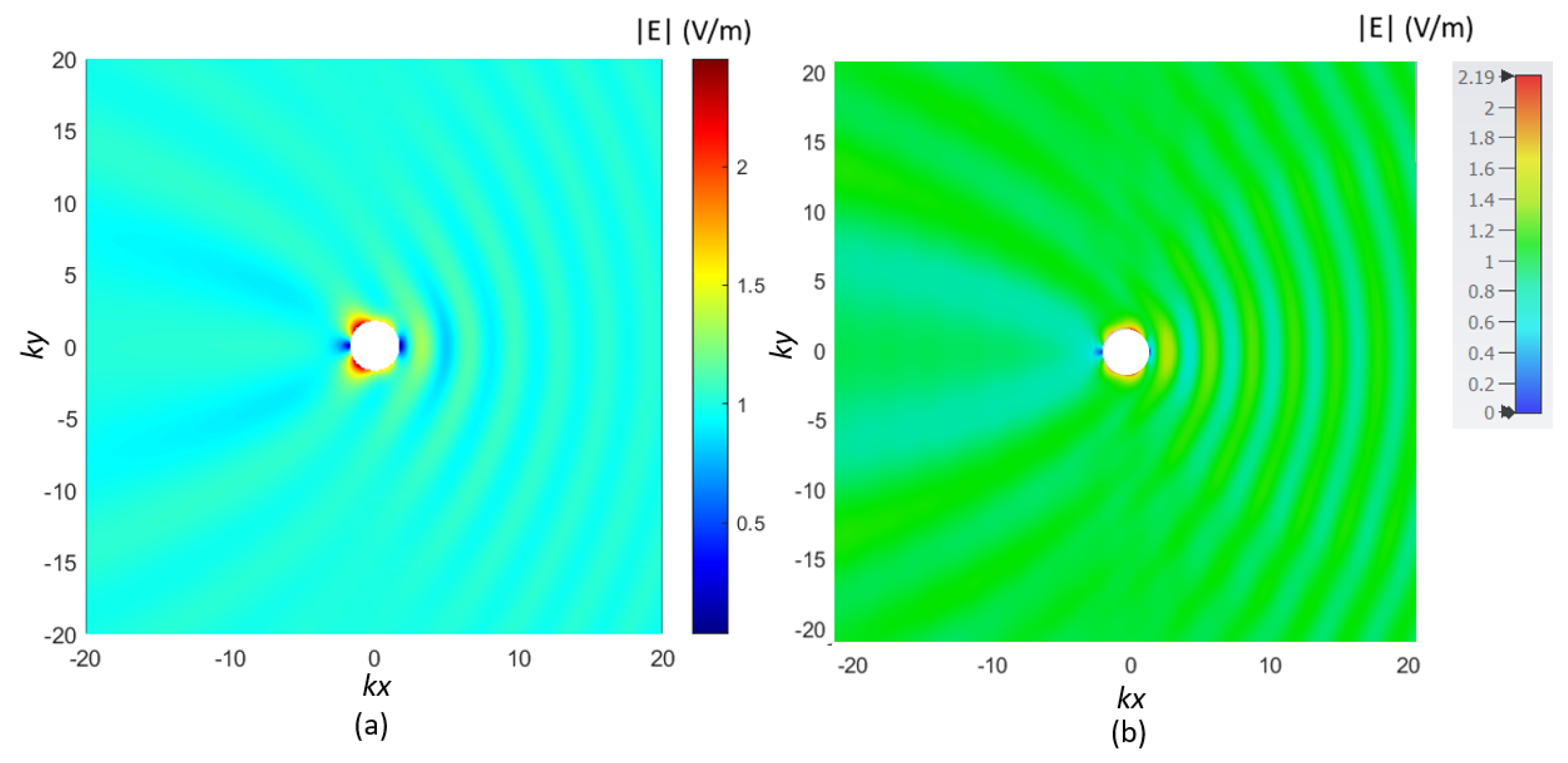
The method was then validated by changing the geometry of the spheroidal scatterer. In fact, two different cases were considered. In the first case, shown in Figure 8, we considered a spheroid with the following parameters: ${\xi }_0=1.01$ and $kd=20$ (corresponding to $ka=10.1$, $kb=1.4177$ and $c=10$). In this case the truncation order was chosen as $m_t=14$ and the $\mathbf{G}$ matrix size was $224\times 224$. It is worth noting that this limiting case could be compared with the case of a 2-D cylindrical geometry scatterer. The comparison between the electric field map across the $xy$ plane in the case of spheroidal geometry of Figure 8 (${\theta }_0={90}^{\circ }$) and that in the case of 2-D cylindrical geometry, obtained with CST, is presented in Figure 9.

The second limiting case is shown in Figure 10 where a spheroid with parameters ${\xi }_0=2$, $kd=2$, $ka=2$, $kb=1.7321$ is considered. In this case the truncation order was $m_t=6$ and the $\mathbf{G}$ size was $48\times 48$. Since the values of interfocal distance $kd$ and c were very small, the spheroid could be approximated by a sphere, the geometry of which represented a limiting case. In fact, in this case, the spheroidal angular and radial functions reduced to spherical Legendre and Bessel functions. The comparison with the case of spherical geometry, obtained with CST, is shown in Figure 11 (${\theta }_0={90}^{\circ }$).

3.2. TM Polarization

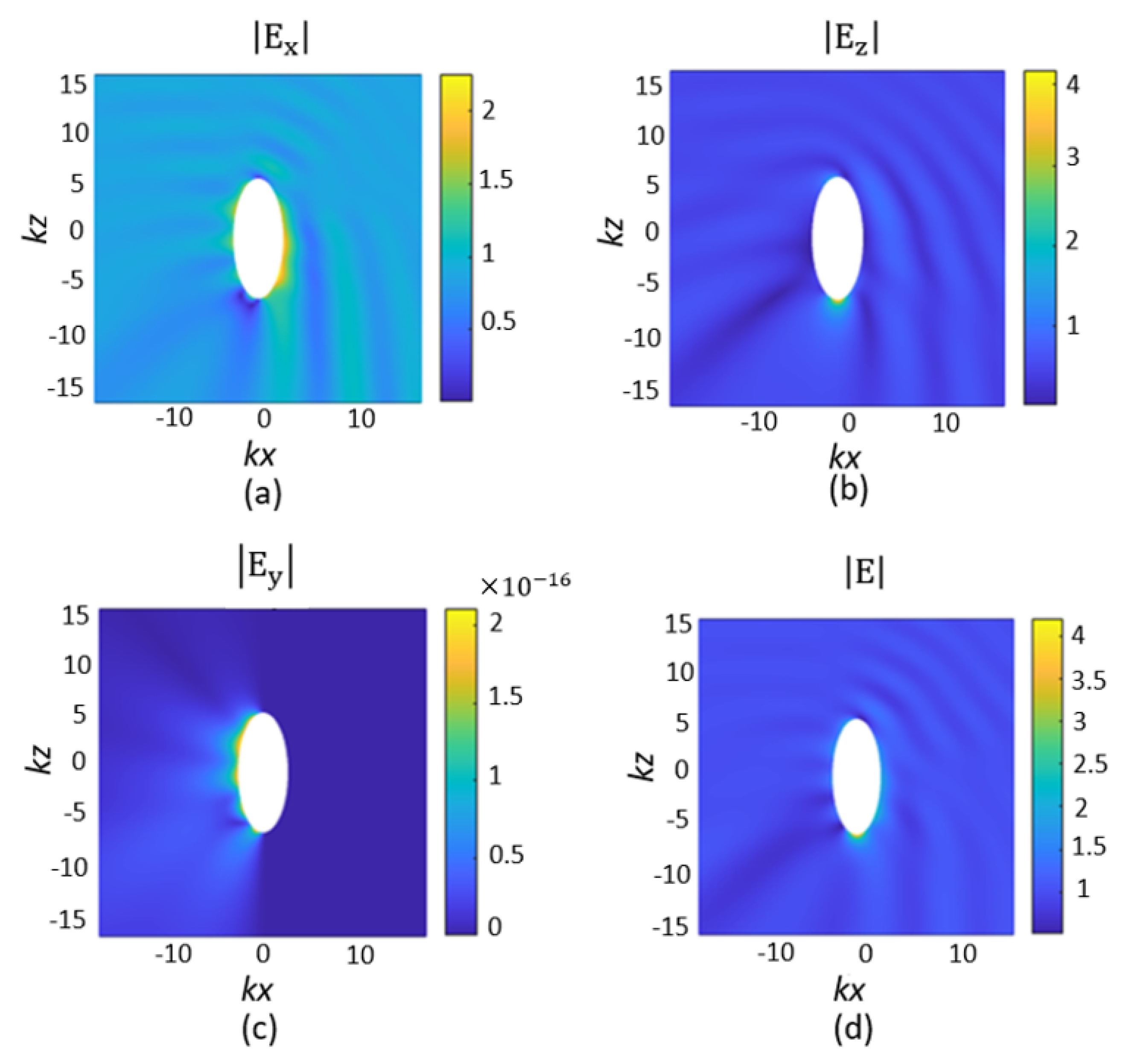
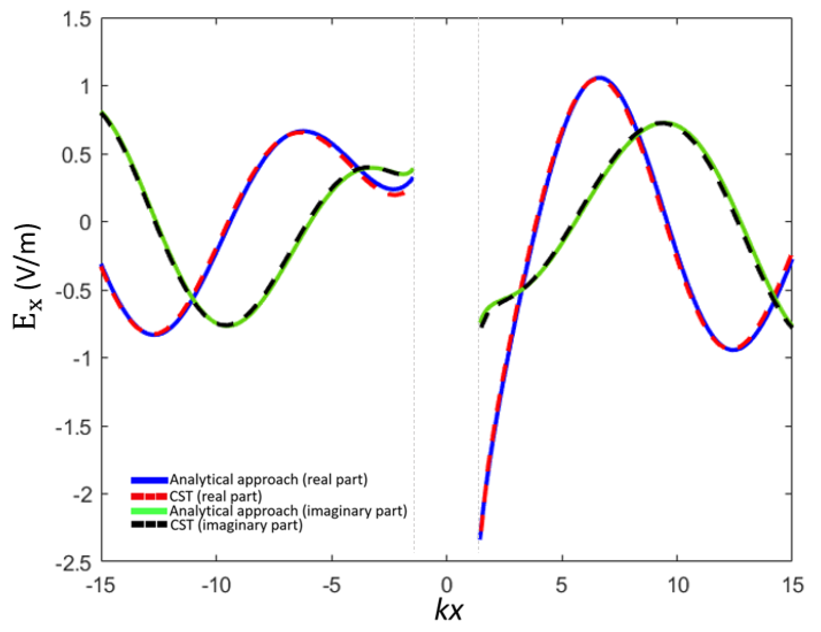
Here we consider the case of TM polarization. In this case the magnetic incident field is perpendicular to the incidence plane. Figure 12 shows the field maps across the $xz$-plane of the electric field. Figure 12a–c show the magnitude of the electric field components $\left|E_x\right|$, $\left|E_y\right|$, $\left|E_z\right|$, respectively. Figure 12d shows the magnitude of the electric field $\left|E\right|$. The geometry of the scatterer is the same in Figure 2. The real and imaginary parts, obtained in both Matlab and CST, of the x- and z-component of the electric field are shown in Figure 13 and Figure 14, respectively.

4. Conclusions

In this paper, we have presented a fast and ad hoc Matlab efficient numerical implementation of the theory of electromagnetic scattering of a plane wave by a conducting ellipsoid of revolution, also known as a spheroid. Numerical results, both for TE and TM polarization and for several propagation directions of the incident wave, have been validated by comparison with the commercial electromagnetic simulator CST Microwave Studio, showing an excellent agreement. To the authors’ knowledge, this is the first time that the libraries used in this work have been used to solve electromagnetic scattering vectorial problems. Truncation criteria were carefully considered. This method, being exact and fast, will allow the development of new analytical techniques that are capable of considering even the presence of a flat interface in the proximity of the spheroidal scatterer, e.g., for applications concerning ground penetrating radar or through-the-wall radar modelling. To this aim, field expansions of spheroidal vector wave functions in terms of plane wave will be considered in future works.

References

- Daniels, D.J. Surface Penetrating Radar, 2nd ed.; IEEE: London, UK, 2004. [Google Scholar]
- Amin, M.G. Through-the-Wall Radar Imaging; CRC Press: New York, NY, USA, 2011. [Google Scholar]
- Fiaz, M.A.; Frezza, F.; Pajewski, L.; Ponti, C.; Schettini, G. Asymptotic solution for a scattered field by cylindrical objects buried beneath a slightly rough surface. Near Surf. Geophys. 2013, 11, 177–184. [Google Scholar] [CrossRef]
- Frezza, F.; Pajewski, L.; Ponti, C.; Schettini, G. Through-wall electromagnetic scattering by N conducting cylinders. J. Opt. Soc. Am. A 2013, 30, 1632–1639. [Google Scholar] [CrossRef] [PubMed]
- Borghi, R.; Santarsiero, M.; Frezza, F.; Schettini, G. Plane-wave scattering by a dielectric circular cylinder parallel to a general reflecting flat surface. J. Opt. Soc. Am. A 1997, 14, 1500–1504. [Google Scholar] [CrossRef] [Green Version]
- Ponti, C.; Vellucci, S. Scattering by conducting cylinders below a dielectric layer with a fast non-iterative approach. IEEE Trans. Microw. Theory Tech. 2015, 63, 30–39. [Google Scholar] [CrossRef]
- Ponti, C.; Tognolatti, L.; Schettini, G. Electromagnetic scattering by metallic targets above a biological medium with a spectral-domain approach. IEEE Open J. Antennas Propag. 2021, 2, 3230–3237. [Google Scholar] [CrossRef]
- Tognolatti, L.; Ponti, C.; Schettini, G. Use of a set of wearable dielectric scatterers to improve electromagnetic transmission for a body power transfer system. IEEE J. Electromagn. Rf Microwaves Med. Biol. 2021. in early access. [Google Scholar] [CrossRef]
- Hansen, W.W. A new type of expansion in radiation problems. Phys. Rev. 1935, 47, 139–143. [Google Scholar] [CrossRef]
- Hansen, W.W. Directional characteristics of any antenna over a plane earth. J. Appl. Phys. 1936, 7, 460–465. [Google Scholar] [CrossRef]
- Hansen, W.W. Trasformations useful in certain antenna calculations. J. Appl. Phys. 1937, 8, 282–286. [Google Scholar] [CrossRef]
- Negishi, T.; Erricolo, D.; Uslenghi, P. Metamaterial spheroidal cavity to enhance dipole radiation. IEEE Trans. Antennas Propag. 2015, 63, 2802–2807. [Google Scholar] [CrossRef]
- Negishi, T.; Erricolo, D. Symmetry properties of spheroidal functions with respect to their parameter. IEEE Trans. Antennas Propag. 2017, 65, 4947–4951. [Google Scholar] [CrossRef]
- Erricolo, D.; Uslenghi, P. Exact radiation for dipoles on metallic spheroids at the interface between isorefractive half-spaces. IEEE Trans. Antennas Propag. 2005, 53, 3974–3981. [Google Scholar] [CrossRef]
- Borrelli, F.; Capozzoli, A.; Curcio, C.; Liseno, A. Numerical results for antenna characterization in a cylindrical scanning geometry using a spheroidal modelling. In Proceedings of the 2021 IEEE International Conference on Microwaves, Antennas, Communications and Electronic Systems (COMCAS), Tel Aviv, Israel, 1–3 November 2021; pp. 230–233. [Google Scholar] [CrossRef]
- Borrelli, F.; Capozzoli, A.; Curcio, C.; Liseno, A. A NFFF approach using spheroidal wave functions in a cylindrical scanning geometry. In Proceedings of the 2021 IEEE International Symposium on Antennas and Propagation and USNC-URSI Radio Science Meeting (APS/URSI), Singapore, 4–10 December 2021; pp. 887–888. [Google Scholar] [CrossRef]
- Li, L.-W.; Yeo, T.-S.; Kooi, P.-S.; Leong, M.-S. Microwave Specific Attenuation By Oblate Spheroidal Raindrops: An Exact Analysis of Tcs’s in Terms of Spheroidal Wave Functions. J. Electromagn. Waves Appl. 1998, 12, 709–711. [Google Scholar] [CrossRef] [Green Version]
- Li, L.-W.; Kang, X.-K.; Leong, M.-S. Spheroidal Wave Functions in Electromagnetic Theory; John Wiley & Sons: Hoboken, NJ, USA, 2004; Volume 166. [Google Scholar]
- Stratton, J.A. Electromagnetic Theory; McGraw-Hill: New York, NY, USA, 1941. [Google Scholar]
- Flammer, C. Spheroidal Wave Functions; Stanford University Press: Stanford, CA, USA, 1957; p. 220. [Google Scholar]
- Moffatt, D.L.; Kennaugh, E.M. The axial echo area of a perfectly conducting prolate spheroid. IEEE Trans. Antennas Propag. 1965, AP-13, 401–409. [Google Scholar] [CrossRef]
- Moffatt, D.L. The echo area of a perfectly conducting prolate spheroid. IEEE Trans. Antennas Propag. 1969, AP-17, 299–307. [Google Scholar] [CrossRef]
- Asano, S.; Yamamoto, G. Light scattering by a spheroidal particle. Appl. Opt. 1975, 14, 29–49. [Google Scholar] [CrossRef]
- Dalmas, J.; Deleuil, R. Multiple scattering of electromagnetic waves from two infinitely conducting prolate spheroids which are centered in a plane perpendicular to their axes of revolution. Radio Sci. 1985, 20, 575–581. [Google Scholar] [CrossRef]
- Dalmas, J.; Deleuil, R. Translational addition theorems for prolate spheroidal vector wavefunctions M’ and N’. Q. Appl. Math. 1986, 44, 213–222. [Google Scholar] [CrossRef] [Green Version]
- Merchant, B.L.; Moser, P.J.; Nagl, A.; Uberall, H. Complex pole patterns of the scattering amplitude for conducting spheroids and finite lenght cylinders. IEEE Trans. Antennas Propag. 1988, AP-36, 1769–1777. [Google Scholar] [CrossRef]
- Jen, L. A dipole antenna embedded in a prolate dielectric spheroid. Sci. Sin. 1962, 11, 173–184. [Google Scholar] [CrossRef]
- Schultz, F.V. Scattering by a Prolate Spheroid; Rep. VMM-42; Willow Run Research Center (University of Michigan): Ann Arbor, MI, USA, 1953. [Google Scholar]
- Reitlinger, N. Scattering of a Plane Wave Incident on a Prolate Spheroid at an Arbitrary Angle; Memo. No. 2868-506-M; Radiation Laboratory (University of Michigan): Ann Arbor, MI, USA, 1957. [Google Scholar]
- Sinha, B.P.; MacPhie, R.H. Electromagnetic scattering by prolate spheroids for plane waves with arbitrary polarization and angle of incidence. Radio Sci. 1977, 12, 171–184. [Google Scholar] [CrossRef]
- Adelman, R.; Gumerov, N.A.; Duraiswami, R. Software for computing the spheroidal wave functions using arbitrary precision arithmetic. arXiv 2014, arXiv:1408.0074. [Google Scholar]
- Fousse, L.; Hanrot, G.; Lefevre, V.; Pellissier, P.; Zimmermann, P. MPFR: A multiple-precision binary floating-point library with correct rounding. ACM Trans. Math. Softw. 2007, 33, 13. [Google Scholar] [CrossRef]
Figure 1.
Prolate spheroid geometry (a) and the spheroidal coordinate system (b).
Figure 2.
Real and imaginary parts of along the x-axis (a) and the z-axis (b): comparison between results obtained through the analytical approach implemented in Matlab and the results obtained through CST Microwave Studio, for the case , , , , , , . TE polarization.
Figure 3.
Magnitude of the E-field across the plane for the same geometrical parameters considered in Figure 2. TE polarization.
Figure 4.
Magnitude of the E-field across the plane for the same geometrical parameters of Figure 2 but for different incident angles of the plane wave: (a) , (b) .
Figure 5.
Validation of the truncation method. Comparison between the results obtained with , , and , to those obtained with : (a) relative error along the x-axis; (b) relative error along the z-axis. TE polarization.
Figure 6.
Amplitude of the elements of the matrix for the case with , , , , , , . All elements with zero value are represented in white.
Figure 7.
Magnitude of the E-field across the -plane for the case of axial incidence (), for the same geometry considered in Figure 2, obtained through the analytical approach in Matlab (a) and through CST Microwave Studio (b). TE polarization.
Figure 8.
Real and imaginary parts of along the x-axis and comparison with the results obtained through CST Microwave Studio (a); magnitude of the E-field across the -plane (b). Used parameters were as follows: , , , , , , . TE polarization.
Figure 9.
Magnitude of the E-field across the -plane: (a) spheroidal geometry with the same geometrical parameters considered in Figure 8 (analytical approach); (b) cylindrical geometry (2-D) (CST Microwave Studio). Cylinder radius was . TE polarization.
Figure 10.
Figure 11.
Magnitude of the E-field across the -plane: (a) spheroidal geometry with the same geometrical parameters considered in Figure 10 (analytical approach); (b) spherical geometry (2-D) (CST Microwave Studio). Sphere radius was . TE polarization.
Figure 12.
Field maps across the -plane for the case of TM polarization for the same case as in Figure 2, the magnitude of the electric field components , , are shown in (a–c), respectively. The magnitude of the electric field is shown in (d).
Figure 13.
Real and imaginary parts of : comparison between the analytical approach implemented in Matlab and CST Microwave Studio, for the geometry of Figure 2. TM polarization.
Figure 14.
Publisher’s Note: MDPI stays neutral with regard to jurisdictional claims in published maps and institutional affiliations. |
© 2022 by the authors. Licensee MDPI, Basel, Switzerland. This article is an open access article distributed under the terms and conditions of the Creative Commons Attribution (CC BY) license (https://creativecommons.org/licenses/by/4.0/).
Share and Cite
MDPI and ACS Style
Tognolatti, L.; Ponti, C.; Santarsiero, M.; Schettini, G. An Efficient Computational Technique for the Electromagnetic Scattering by Prolate Spheroids. Mathematics 2022, 10, 1761. https://doi.org/10.3390/math10101761
AMA Style
Tognolatti L, Ponti C, Santarsiero M, Schettini G. An Efficient Computational Technique for the Electromagnetic Scattering by Prolate Spheroids. Mathematics. 2022; 10(10):1761. https://doi.org/10.3390/math10101761
Chicago/Turabian StyleTognolatti, Ludovica, Cristina Ponti, Massimo Santarsiero, and Giuseppe Schettini. 2022. "An Efficient Computational Technique for the Electromagnetic Scattering by Prolate Spheroids" Mathematics 10, no. 10: 1761. https://doi.org/10.3390/math10101761
Note that from the first issue of 2016, this journal uses article numbers instead of page numbers. See further details here.