Assessing the Relevance of Information Sources for Modelling Student Performance in a Higher Mathematics Education Course

Abstract

In recent years, most educational institutions have integrated digital technologies into their teaching–learning processes. Learning Management Systems (LMS) have gained increasing popularity, particularly in higher education, due to their ability to manage teacher–student interactions. These systems store valuable information which describes students’ behaviour throughout a course. These data can be utilised to construct statistical models that represent learner behaviour within an online LMS platform. In this study, we aim to compare different sources of information and, more ambitiously, to provide insights into which source of information is most valuable for inferring student performance. The considered sets of information come from (i) the Moodle LMS; (ii) socio-economic data about students acquired from a survey; and (iii) subject marks achieved throughout the course. To determine the relevance of the incorporated information, we use artificial intelligence (AI) methods, and we report the importance measures of four state-of-the-art methods. Our findings indicate that the selected methodology is suitable for making inferences about student performance while also shedding light on model decisions through explainability.

1. Introduction

Improving the quality of education is a crucial objective for achieving sustainable development, as recognised by the United Nations in its fourth Sustainable Development Goal (https://www.un.org/sustainabledevelopment/education/ (accessed on 15 May 2023)). Access to quality education is essential for enhancing people’s lives and promoting sustainable development. A primary objective related to higher education is to ensure access to affordable technical, vocational, and higher education, as well as to expand scholarships for developing countries in these fields.

In particular, mathematics has garnered special attention due to its cross-disciplinary nature and connections with teaching–learning methodologies such as STEM education [1], which emphasises Science, Technology, Engineering, and Mathematics. Mathematics plays a critical role in Computer Science programs in higher education. Specifically, it serves as one of the core foundations for developing theories and methods in computer and information sciences. The formalism and logical language of mathematics are instrumental in fostering computational reasoning and thinking.

In recent years, Learning Management Systems (LMSs) have been widely adopted by universities. As a result of the COVID-19 pandemic, many face-to-face courses transitioned to fully online or blended learning [2] environments, guided by educational, hygienic, and/or political considerations. This shift in educational paradigms has substantially impacted the conventional approaches to teaching, learning, and interaction for both teachers and students.

The cornerstone of educational technology is the Learning Management System (LMS). It is typically an online platform designed to organise, invigorate, mentor, assess, manage, and administer learning activities [3]. Its primary responsibilities include managing users (students, teachers, and administrators), resources, and activities, as well as monitoring the educational process through assessments and reports. Furthermore, it equips members of the educational community with communication tools such as internal messaging, chats, video conferencing, forums, and more. By utilising such a virtual platform, teachers and students can benefit from accessing and sharing a unified information source. Figure 1 provides a visual representation showcasing the various functions of a standard LMS.

In recent educational research, the subject of student performance analysis and prediction has attracted considerable attention [3,5,6]. Traditionally, inferences about student grades have been made using various offline data sources, such as student grades, demographics, social, and school-related characteristics, primarily collected through school reports. This methodology is demonstrated in [7]. The use of LMS has introduced the incorporation of student data obtained through an online platform when examining student behaviour throughout the course, including aspects such as activity, platform engagement, assistance, and assessments.

The current era is predominantly defined by technological developments such as computers and intelligent mobile phones, fueled by the vast number of data collected and generated by both humans and machines [4]. These technological tools driven by data are closely intertwined with advancements in mathematics. Increasing success in higher education, particularly in mathematics, is of crucial importance [8].

Computer tools, such as data logging systems, graphing tools, simulation, and modelling environments, can also influence learning by facilitating changes in classroom interactions [9]. The information captured by these systems has been shown to be useful in describing students’ behaviour [6,10]. Furthermore, the study by [4] emphasises the importance of user interactions on LMS platforms for obtaining relevant information about students. Despite the breadth of literature on this topic, we found that most works focus on the stored information within LMSs [11]. This line of study has received special attention [12] with the advent of Artificial Intelligence. Moreover, it has been extensively investigated [13] to gain a better understanding of student behaviour and to design appropriate educational environments that facilitate the teaching–learning process.

In [14], the authors discuss the limitations of certain electronic learning environments and advocate for math-friendly systems that allow for the exchange of mathematics diagrams and notation between instructors and students. The study concludes that learning difficult concepts in these math-friendly environments is comparable to doing so in face-to-face courses. We recognize the importance of using such math-friendly environments and have opted to utilize the Moodle Learning Management System (LMS), which supports the use of LaTeX (https://www.latex-project.org (accessed on 15 May 2023)) for sharing diagrams with students. LaTeX has proven to be the predominant language for document preparation in the scientific community, particularly in the field of mathematics, due to its compatibility with mathematical symbols and syntax. The use of multimedia sources has also been demonstrated to be effective in mathematics education. For example, in [15], the authors employed an interactive, multimedia-based instructional system in a mathematics methods class for pre-service elementary school teachers. Their findings revealed that students were more likely to integrate knowledge acquired from the system into their teaching methods compared to conventional approaches. LMSs have also proven to be valuable tools during the COVID era [16], where teachers confronted the complexities of online instruction and developed innovative forms of collaborative work.

In this study, we investigate three different sources of information to make inferences about student performance through artificial intelligence (AI) models. Specifically, we examine three distinct approaches. Firstly, we used purely LMS-generated data from the platform collected in the course log-file. We adopted the methodology recently proposed in [6]. This information is based solely on activities conducted within the LMS and encompasses data in the Event Name and Event Context columns of the log-file. It quantifies students’ interaction in terms of activities, file downloads, forum participation, class attendance, and more. For further details, see

Table 1. Feature number and description, containing information about the 38 features extracted from the Moodle LMS according to [6].

#	Description	#	Description
1	A file has been uploaded	20	Quiz attempt submitted
2	A submission has been submitted	21	Quiz attempt summary viewed
3	Badge listing viewed	22	Quiz attempt viewed
4	Calendar event created	23	Remove submission confirmation viewed
5	Calendar event deleted	24	Scheduler booking added
6	Comment created	25	Scheduler booking form viewed
7	Comment deleted	26	Scheduler booking removed
8	Course module instance list viewed	27	Step shown
9	Course module viewed	28	Submission created
10	Course user report viewed	29	Submission form viewed
11	Course viewed	30	Submission updated
12	Grade overview report viewed	31	Status’ submission has been updated
13	Grade user report viewed	32	Status’ submission has been viewed
14	Group deleted	33	Tour ended
15	Group member added	34	Tour started
16	Group member removed	35	User graded
17	Group updated	36	User list viewed
18	Quiz attempt reviewed	37	User profile viewed
19	Quiz attempt started	38	Zip archive of folder downloaded

. Secondly, we used data acquired from a survey that gathers socio-economic features of students. We adapted the survey proposed in [7]. The set of features collected in the survey is detailed in

Table 2. Socio-economic features extracted from an adapted survey [7].

#	Name	Detailed Description
1	gender	student’s gender (male, female, other)
2	age	student’s age
3	address	student’s home address type (urban or rural)
4	famsize	family size
5	Pstatus	parent’s cohabitation status
6	Medu	mother’s education
7	Fedu	father’s education
8	Mjob	mother’s job
9	Fjob	father’s job
10	reason	reason for choosing this university
11	guardian	student’s guardian
12	traveltime	home-t0 faculty travel time
13	studytime	weekly study time
14	failures	number of past class failures
15	famsup	family educational support
16	paid	extra paid classes within the course subject
17	activities	extra-curricular activities
18	higher	wants to take higher education (post-grade)
19	romantic	with a romantic relationship
20	famrel	quality of family relationships
21	freetime	free time after school
22	goout	going out with friends
23	Walc	weekend alcohol consumption
24	health	current health status
25	absences	number of school absences

. Finally, we used students’ marks generated during the course, which contribute to their final course grades. In-depth information about the marks can be found in

Table 3. Student performance throughout the Computer Science course in the Mathematics degree, as indicated by their grades.

Number	Detailed Description
1	Classroom works mark
2	Exam mark
3	Videos’ mark
4	Seminars’ mark
5	Practicals’ marks
6	Voluntary homework’s marks

. By analysing these information sources, we aim to better understand and predict student performance in educational settings.

The remainder of this work is organised as follows. Section 2 reviews the materials and methods used in the present study. It offers insights into the AI methods used to make inferences about students’ performance and their corresponding model interpretation. Additionally, it explains the data acquisition and harmonisation procedure. Section 3 presents an exhaustive description of the experiment and the results achieved, along with their interpretation. Finally, in Section 3 provides the concluding remarks and some suggestions for possible extensions of our work.

2. Materials and Methods

This section elaborates on the statistical learning methodology employed in the experimental setup, offering a broad comparison across four different methods utilised in the machine learning field. Furthermore, it delves into the details of the data set designed specifically for this study. In particular, we provide a comparison among data generated from the Moodle LMS, a socio-economic survey, and students’ marks achieved in the subject. In our study, we propose applying the artificial intelligence techniques in order to exploit the LMS-generated data [13]. This combination of AI and educational data exploitation has acquired relevant interest in the Educational area [12].

2.1. Statistical Learning Models

In this section, we outline the various methods employed in the experimental Section 3, along with the metrics used to measure their performance.

In particular, we used four state-of-the-art methods for predicting student performance in the teaching subject of computer science within the Mathematics degree at the University of València. We considered these four models due to their strong performance in regression tasks and their ability to provide understandable explanations for their decisions through model weight inspection. These models are the Gaussian Processes regression (Section 2.1.1) (GP), a powerful nonlinear model; the Partial Least Squares (Section 2.1.2) (PLS), a model useful in small sample size problems and robust to multicollinearity [17]; LASSO (Section 2.1.3), a model that yields a sparse representation; and Ridge Regression (Section 2.1.4) (RR).

In the following, we consider a data set $\mathcal{D}$ of n observations,

$$\mathcal{D}=\left\{({\mathbf{x}}_i,y_i)\in {\mathbb{R}}^{d\times 1}|i=1,\dots ,n\right\},$$

where the d-dimensional input vector ${\mathbf{x}}_i$, referred to as the feature vector, contains a representative set of d features representing the i-th student, and the output scalar $y_i$ represents the associated student’s mark in the subject. The goal of our work is to fit a model f between input feature vector ${\mathbf{x}}_i$ and the corresponding output value $y_i$, i.e., $f\left({\mathbf{x}}_i\right)=y_i,i=1,\dots ,n$. One advantage of this model is its ability to make inferences on a new, unseen feature vector ${\mathbf{x}}^{*}$ through $f\left({\mathbf{x}}^{*}\right)$. Recent AI techniques rely on the Empirical Risk Minimisation principle and provide risk guarantees through Statistical Learning principles, which offer statistical guarantees and good performance in model fitting [18,19]. All the methods used in this study are based on this theory and are revisited below.

2.1.1. Gaussian Process Regression

Gaussian Process Regression (GPR) [20] is a probabilistic model that offers a nonlinear least squares regression model through the use of kernel methods [21]. Specifically, we used the Automatic Relevance Determination (ARD) kernel covariance function,

$$k_{ARD}({\mathbf{x}}_i,{\mathbf{x}}_j)=exp\left(-\frac{1}{2}{({\mathbf{x}}_i-{\mathbf{x}}_j)}^{\top }{\mathrm{\Sigma }}^{-1}({\mathbf{x}}_i-{\mathbf{x}}_j)\right),$$

(1)

where $\mathrm{\Sigma }$ is a diagonal matrix with a diagonal composed of $\{{\sigma }_1^2,\dots ,{\sigma }_d^2\}$ parameters to weigh each input dimension. The ARD kernel is a natural extension of the Radial Basis Function (RBF) with only one parameter, as it weighs each feature independently (the scale factor is ignored in both covariance functions for the sake of convenience). For a comprehensive understanding of the model formulation and a broader study of Gaussian Processes theory, refer to [20]. One advantage of using the ARD kernel is that it allows for estimates of the importance of each variable. In particular, we define the importance measure of the i-th input feature ($1\le i\le d$) as the $\frac{log\left({\sigma }_i^2\right)}{{\sum }_{j=1}^d{\sigma }_j^2}$. This measure reveals the importance assigned to the i-th input feature by the GP model.

We choose this method for several reasons. First, it is nonlinear and provides robust estimations when the relationship between input and output data is nonlinear. Second, since it is based on a probabilistic approach, it offers confidence intervals for inferred values. Third, the ARD kernel allows for the establishment of an importance ranking for input features, shedding light on the model behaviour during the inference process.

2.1.2. Partial Least Squares

Partial Least Squares [22] (PLS) is a statistical method that finds a linear regression model by projecting the predicted variables and the observable variables onto a new space. The PLS model seeks to identify the multidimensional direction in the input space of X (formed by the input vectors) that accounts for the maximum multidimensional variance direction in the output space (formed by the values in y). PLS regression is particularly suitable when the predictor matrix has more variables than observations ($d>n$) and when there is multicollinearity [17] among the input variables.

In summary, the PLS model is advantageous when there are more dimensions than input samples. Moreover, it is well-suited to deal with multicollinearity, which refers to the presence of highly correlated input features.

All models have been statistically trained through the leaving-one-out procedure [23] (LOO), a robust statistical technique with theoretical guarantees. This technique selects one sample for model testing and uses remaining samples for model building. Once the model is trained with the $n-1$ samples, it is tested over the remaining samples. This process is repeated n times by permuting the sample, and the final averaged error is provided.

2.1.3. LASSO

Some models are considered black-box models as they do not provide information about their decision-making process. One approach to circumvent this issue is to examine the model weights, which express the importance or relevance of the input variables in the inference process. We propose using L1-constrained linear least squares fits [24] (LASSO). LASSO is a least squares problem formulation with an L1 penalty term applied to the model weights. This method enforces sparsity on the model weights, aiming to set non-relevant features in the input data to zero. Consequently, this allows for a clearer representation of which input features are relevant when the model performs inferences.

2.1.4. Ridge Regression

The method of least squares regression (LS) is a standard inference technique. It utilises a data matrix $\mathbf{X}\in {\mathbb{R}}^{\mathbf{n}\times \mathbf{d}}$, containing real-valued observed variables. Here, n represents the total number of samples, and d is the number of variables or covariates in the study. The goal is to make inferences about another variable $\mathbf{y}\in {\mathbb{R}}^{\mathbf{n}}$ through linear model weights $\mathbf{w}\in {\mathbb{R}}^{\mathbf{d}}$. In this case, the estimated output variable is $\widehat{\mathbf{y}}=Xw$. One of its limitations arises in the presence of multicollinearity when some input variables are correlated, which is the case in our study. Several alternatives exist to address this issue, one of the most accepted being Ridge Regression (RR). In the context of multicollinearity, standard linear regression may result in poor estimates. To overcome this, a regularisation term can be added to the original least squares problem, known as Tikhonov regularisation, which leads to ridge regression. The regularisation term can be adjusted to match the amount of noise in the input data.

2.2. Data-Set Harmonisation

In this section, we describe the three different sources of information: the Moodle (https://moodle.org/ (accessed on 15 May 2023)) LMS, a survey capturing students’ socio-economic characteristics, and scores obtained in various tasks such as homework and coursework.

Our student sample consists of a full course of computer science within the mathematics degree. In particular, the study was developed with a total of 18 students in a first-semester course ranging from September to December of 2022.

2.2.1. Moodle Log-File Data

We adopted the methodology proposed in [6] to extract an informative set of variables from the Moodle platform throughout the subject. This approach is effective for obtaining activity data generated on the online LMS platform. It involves creating occurrence matrices from the raw log-file of the online course by counting the amount of activity generated by each student in terms of the Event Name and Event Context components. The former, Event Name, pertains to activities such as questionnaires or quizzes proposed by the teacher, while the latter, Event Context, refers to Moodle’s internal categorisation of the created Event Name.

Table 1 presents the 38 features exhibiting activity during the mathematics course within the mathematics degree. In a log-file, the LMS sequentially stores raw log data. Event observers are unable to alter event data or stop the dispatching of events since the communication connection is one-way. The variables that Moodle stores serve as the primary source of data for the inference procedures that are taken into consideration in this study. The raw Moodle log-file, which is kept in plain text format, is specifically made up of a series of user-performed events. This log file only records a student’s activities within a course; it excludes other log data, such as internal system mistakes. As a result, it offers a wealth of data that may be used to identify and describe student activities throughout the teaching–learning process. In particular, the information used has been shown to comprise practical variables to aid in inference [5,6,25].

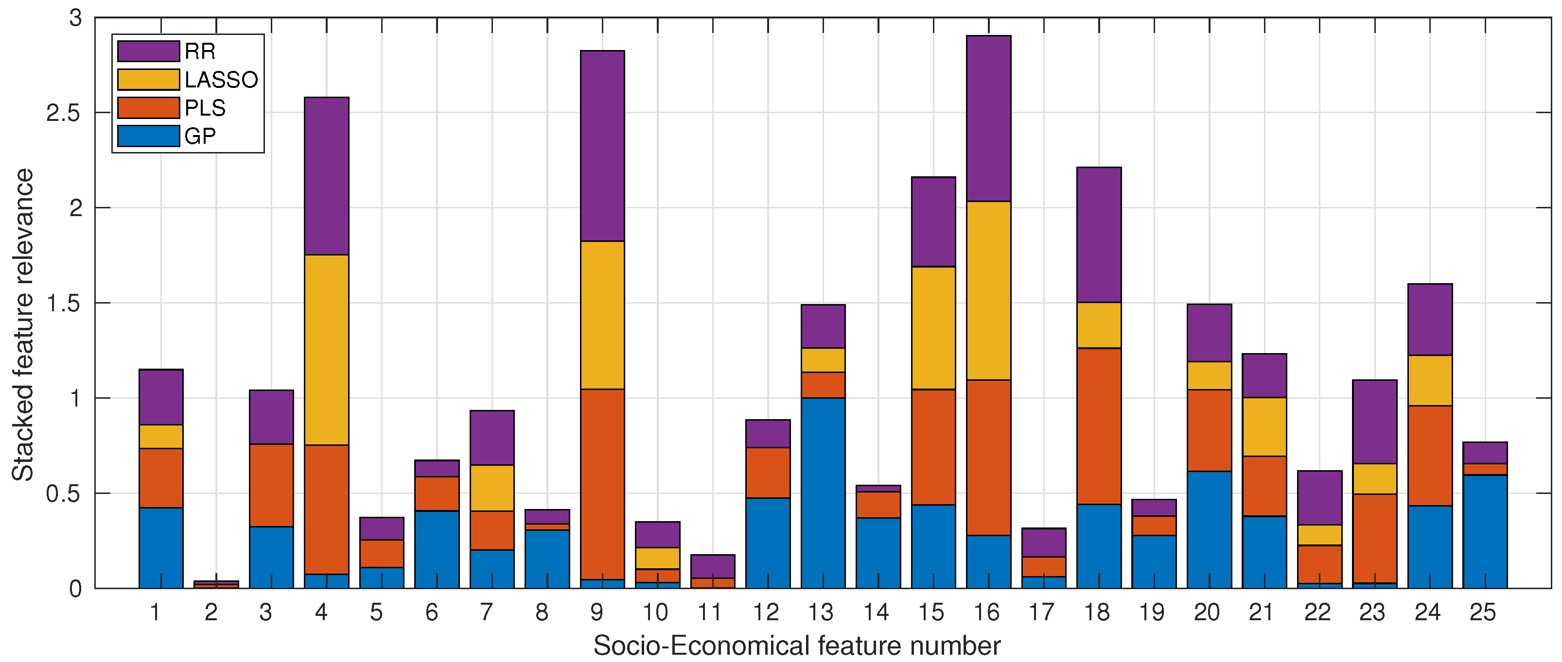
2.2.2. Socio-Economic Data

Table 2 displays the various features used to describe the socio-economic aspects of the student population in this study. We administered a test comprising 29 features, as outlined in [7]. Specifically, the attributes from 2 to 30 can be found at the url cited therein (https://archive.ics.uci.edu/ml/datasets/student+performance (accessed on 15 May 2023)). For the sampled students, certain variables remained constant, such as the lack of extra educational support (schoolsup) received by any of them, the absence of attendance at nursery school (nursery), the presence of internet access at home (internet) for all, and no alcohol consumption on workdays (Dalc). These data were obtained through a survey administered to the students.

2.2.3. Course Marks

To fully investigate the topic at hand, we examine the impact of student performance throughout the course. In particular, we consider the grades presented in Table 3, which include marks for classroom assignments, exams, seminars, practicals, and voluntary homework.

3. Experiments and Results

3.1. Correlation Analysis

In this section, we analyse the correlation between input variables, as well as the correlation between input variables and the output variable.

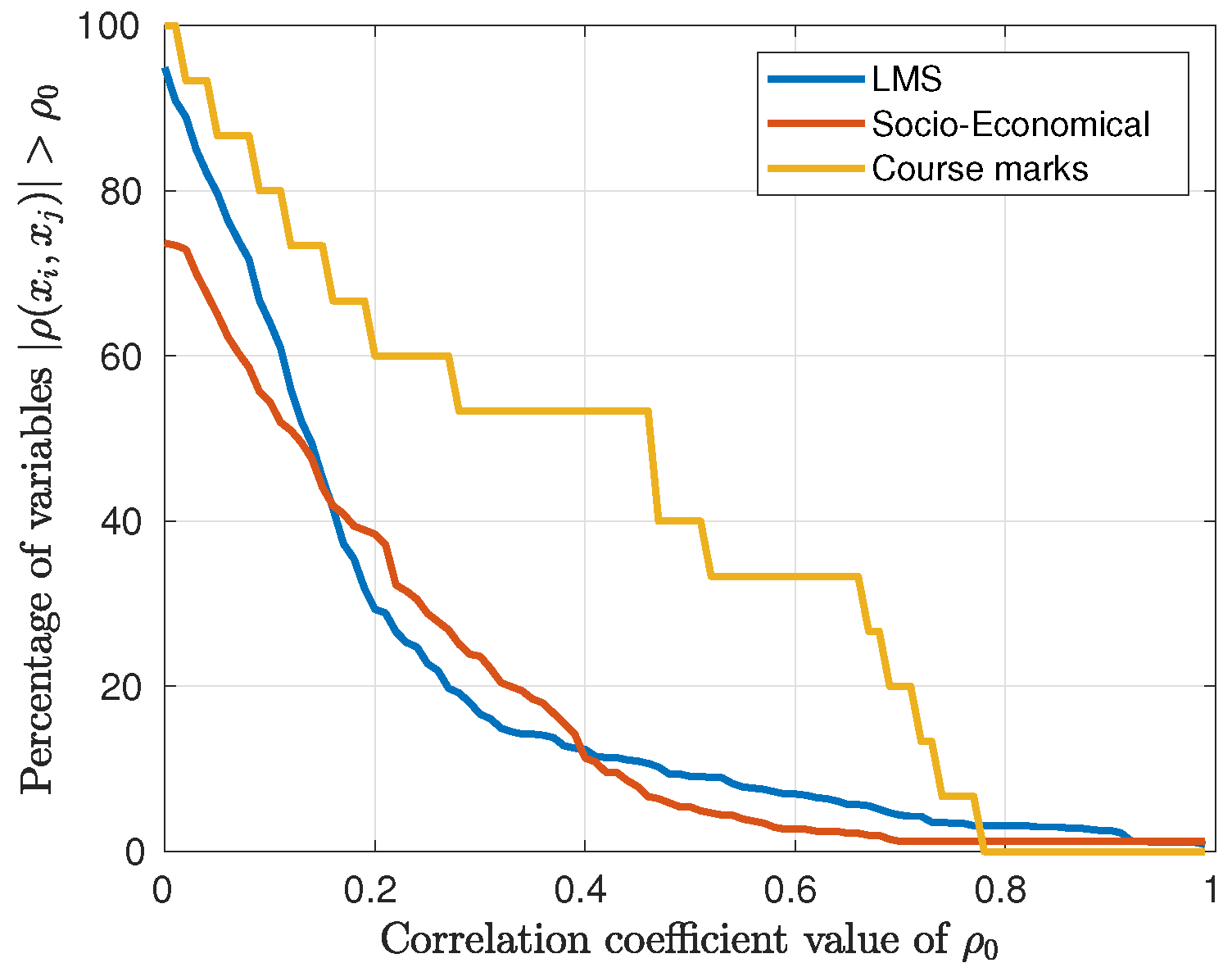
3.1.1. Correlation between Input Variables

We computed the correlation between observed variables within each data set source separately. Recall that we have three different sources of information: Moodle LMS, socio-economic data, and subject marks.

Our data correlation study detected multicollinearity, which refers to the presence of high-correlation coefficients $\rho$ between variables. We consider the Pearson correlation coefficient [26] to measure the correlation between two variables $x,y$ as shown in the equation

$$\rho =\frac{{\sum }_{i=1}^n(x_i-\overline{x})(y_i-\overline{y})}{\sqrt{{\sum }_{i=1}^n{(x_i-\overline{x})}^2}\sqrt{{\sum }_{i=1}^n{(y_i-\overline{y})}^2}}.$$

We deliberately chose the above-proposed method due to its robustness under the assumption of multicollinearity among input variables. Multicollinearity occurs when one predictor variable in a multiple regression model can be linearly predicted from the others with a high degree of precision. In this case, minor adjustments to the model or the data may result in unpredictable changes in the coefficient values of the multiple regression changing. However, in our sample data set, multicollinearity only affects computations related to specific variables and does not impact the overall predictive potential or reliability of the model. We also included results in terms of the Spearman’s rank correlation coefficient [27] $r_s={\rho }_{R\left(x\right),R\left(y\right)}$, where the n raw scores $x_i,y_i$, with $1\le i\le n$, are converted to ranks $R\left(x_i\right),R\left(y_i\right)$. This means that $r_s\in [-1,1]$ provides the highest values (recall that it is bounded by 1) if higher values in x corresponded with higher values of y.

Figure 2 represents the percentage of input variable pairs $x_i,x_j,1\le i,j\le n$ that exhibit a correlation $|\rho (x_i,x_j)|>{\rho }_0,$ for a fixed value of ${\rho }_0\in [0,1]$. This provides an indication of the number of correlated variables for a given threshold ${\rho }_0$. At a threshold of ${\rho }_0=0.2$, the LMS and socio-economic data sets display a correlation of around 40% of variables. However, the proportion of variables with a correlation value above ${\rho }_0>0.5$ is less than 10% in these data sets. The course marks data set, which is the smallest, shows a slower decay of the correlation values but also exhibits a relatively low proportion of correlated variables.

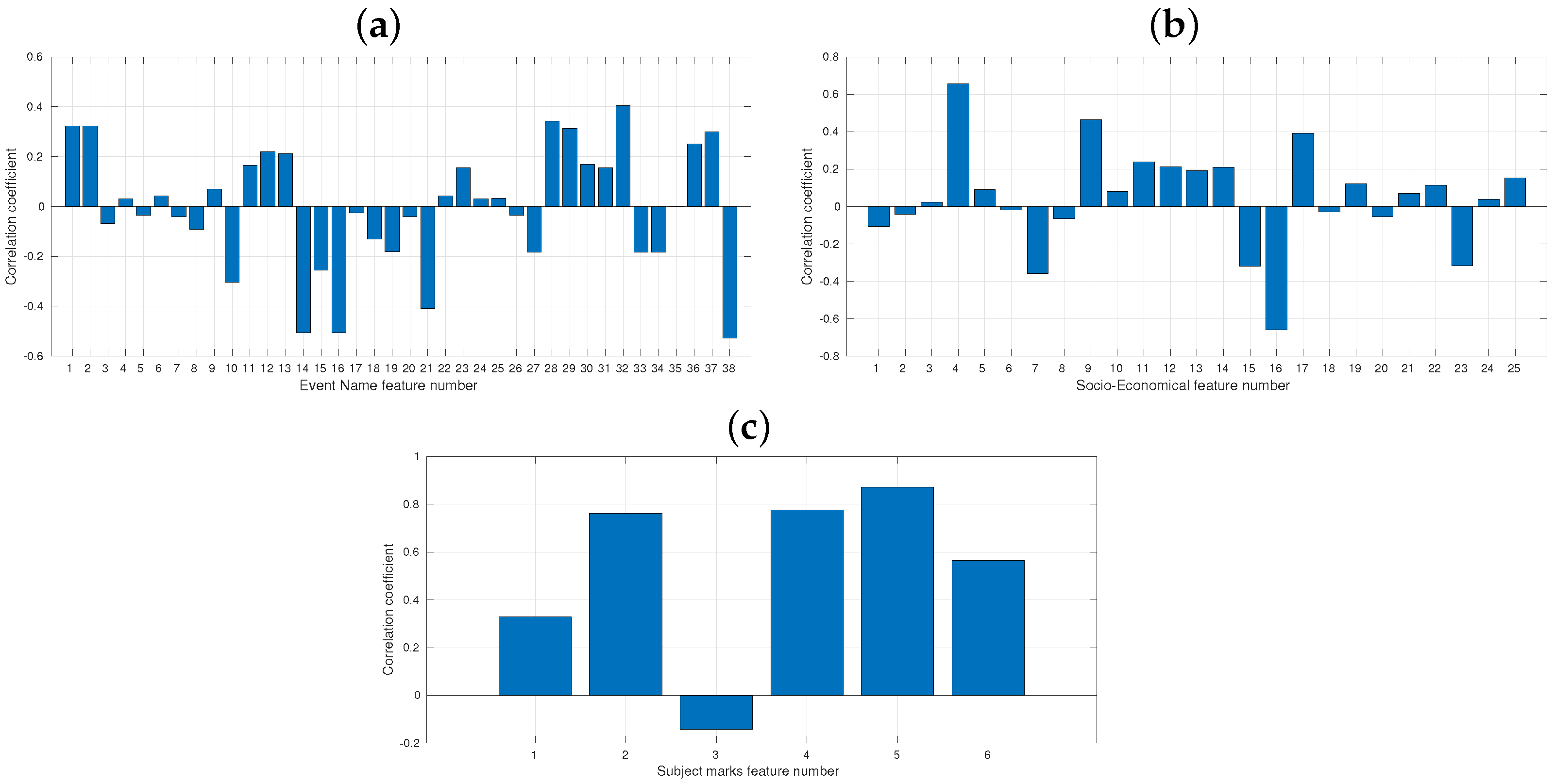
3.1.2. Correlation between Inputs and Output Variable

Before studying the correlation between the input variables and the output variable, we will provide some information about the marks (the output variable). Figure 3 illustrates the kernel density estimation of the students’ final marks. It is visually evident that most of the students passed the subject. Around 2% had a score of 3 (out of a maximum of 10), while there was a peak around the 8.5 mark value, indicating the good performance of the students in the subject.

Figure 4 illustrates correlations between the input variables and the output variable, the students’ final course mark y. In Figure 4a, the correlations of LMS variables with y are presented. The variables with the highest negative correlation coefficients are 14, 16, 21, and 38, with $\rho$ values around −0.5. These variables correspond to Group deleted, Group member removed, Quiz attempt submitted, and Zip archive of folder downloaded, respectively (refer to Table 1). The variable with the highest positive correlation coefficient is 32, corresponding to Status’ submission has been viewed. In Figure 4b, the correlations of socio-economic variables with y are shown. The two variables with the highest correlation coefficients are variable 4 (Family size), with a coefficient over 0.6, and variable 16 (Extra paid classes), with a negative coefficient (refer to Table 2). In Figure 4c, the correlation among the students’ course marks is shown, with a total of four out of six variables achieving relatively high correlation coefficients, with values over 0.7 with the output variable y (refer to Table 3).

3.2. Feature Ranking Analysis

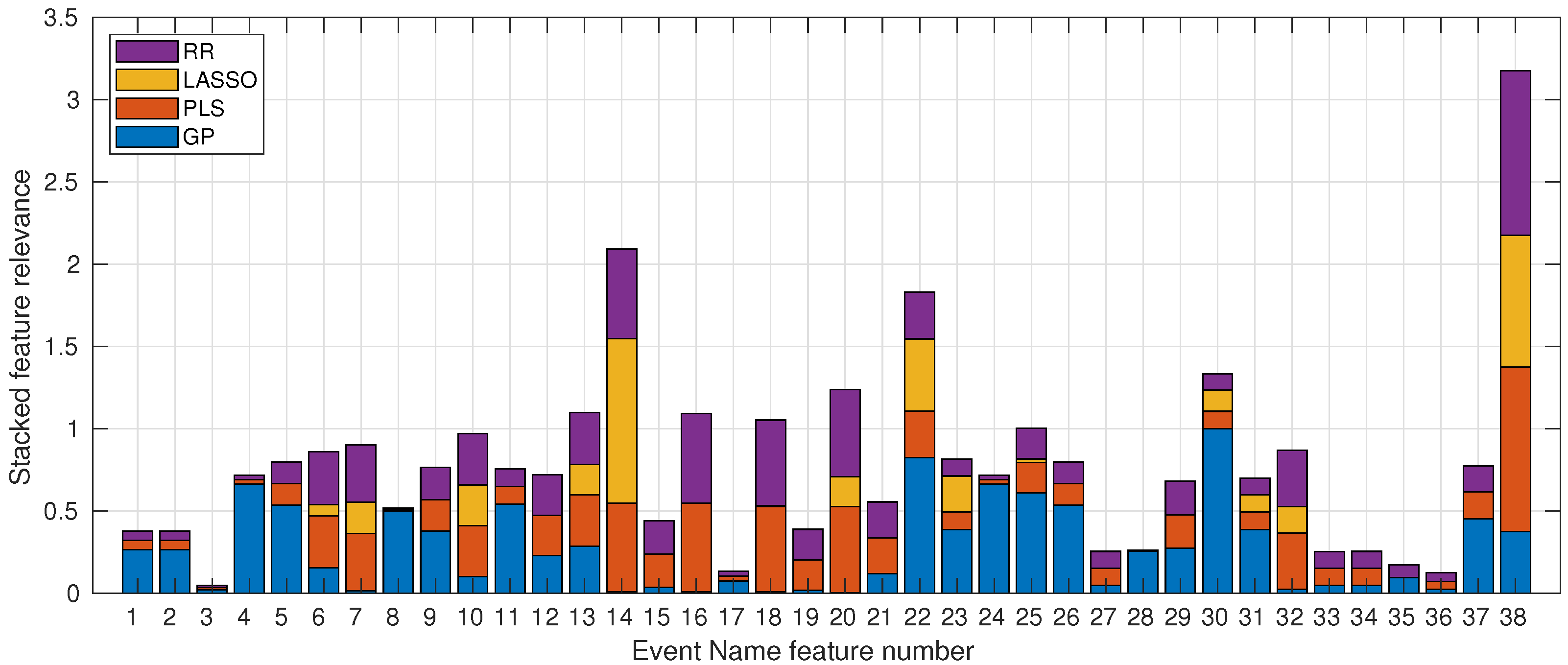
One of the key features of machine learning (ML) methods is their ability to be interpreted as black-box models [28]. Black-box models are systems or processes that can be constructed based solely on their inputs and outputs, without any understanding of how they operate internally. However, the proposed ML models can be interpreted through the inspection of their weights, which provides information about the relevance of the variables in the final trained model [29]. In the following sections, we provide the weights of the models in absolute value and normalised form for the PLS, LASSO, and RR methods. For the GP method, the values of the kernel ARD (see Equation (1)) are transformed to $|log{\sigma }_i^2|$ and then normalised to sum up to 1. We provide a detailed study of the weights of the models, as they contain valuable information about the relevance of the variables in the final trained model.

3.2.1. Moodle LMS

Figure 5 shows a stacked bar plot of the four different models applied to the Moodle LMS dataset. Each color represents one of the proposed methods, from bottom to top: GP, PLS, LASSO, and RR. The four most relevant features are numbers 38, 14, 22, and 30, based on the highest bars achieved by the four methods. These correspond to Zip archive or folder downloaded, Group deleted, Quizz attempt viewed, and Submission updated, respectively (see Table 1). Most of them are related to the activity of the students along the Moodle platform, particularly downloading and resolving tasks and quizzes, which quantify the continuous evaluation of students and are the most relevant features for the inspected models.The most balanced features among the methods coincide with the first and third most relevant features, numbers 38 and 22. It is worth noting that the GP considers the second most relevant feature, number 14, to be the least relevant, which is related to system maintenance tasks. The least weighted features are 3, 17, and 36, which refer to Badge listing viewed, Group updated, and User list viewed, respectively. These features are related to student inspection of lists about the course, such as seeing the rest of the students. It seems reasonable that inspecting lists does not affect the final student mark as much as interacting with the continuous evaluation tasks mentioned above. Among the proposed methods, only the LASSO model enforces sparsity on the weight models through the minimisation of the L1-norm. As can be seen visually, the LASSO bars are usually smaller than the bars of other methods and take values of zero or closer to zero in most cases.

3.2.2. Socio-Economic Data

Figure 6 displays the weights of the features that are related to the socio-economic survey, as calculated by the models used in this study. Notably, the top five most relevant features (i.e., those with the highest bars) are features 16, 9, 4, 18, and 15, respectively. These numbers correspond to extra paid classes, father’s job, family size, and family education support, as listed in Table 2. It is interesting to observe that both extra academic support and family education support are deemed relevant by the models. Additionally, variables related to family, such as the father’s job and family size, appear to influence the model’s predictions. While the study time variable (number 13) did not make it to the top five, it still received a relatively high score in terms of its relevance.

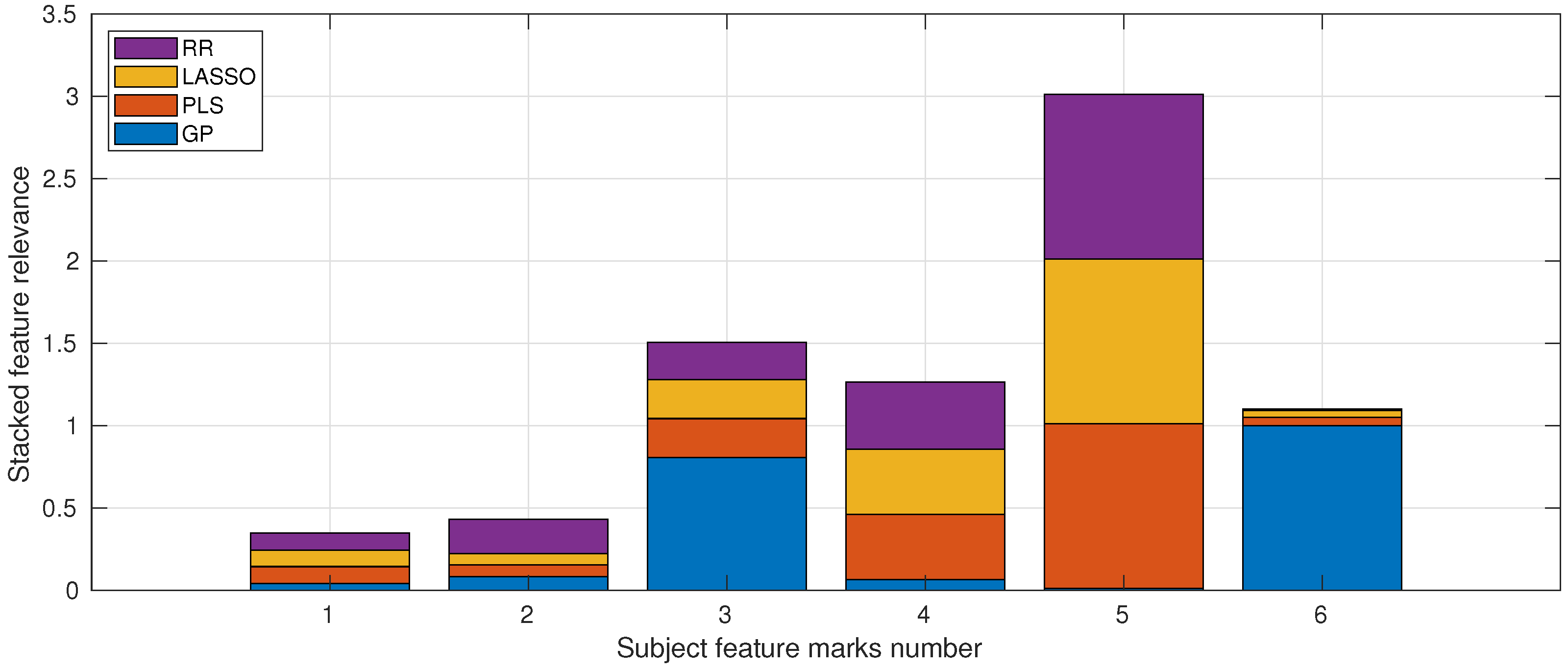
3.2.3. Subject’s Marks

In each particular subject course, there is a categorisation of marks that ultimately contribute to the final grade earned. These marks have been presented in Table 3. Our aim is to identify the most significant source of marks for the models under consideration.

Figure 7 depicts the weights attained by the models. The Practical marks feature attained the highest weight, followed by the Video marks and the Seminar marks, corresponding to features 5, 3, and 4, respectively. Notably, the GP method attributed less weight value to the Practical marks and more to the Video marks and Voluntary Homework marks.

As a concluding remark to this experiment, analyzing the models’ weights provides valuable insights into the factors that have the greatest impact on students’ final marks. This quantitative approach can be useful in comparing different methodologies and evaluation strategies and in designing and validating them. Thus, the present experiment has shed light on the importance of different parts of the methodology in determining students’ marks and has highlighted the significance of factors such as practices, videos, and seminars in this regard.

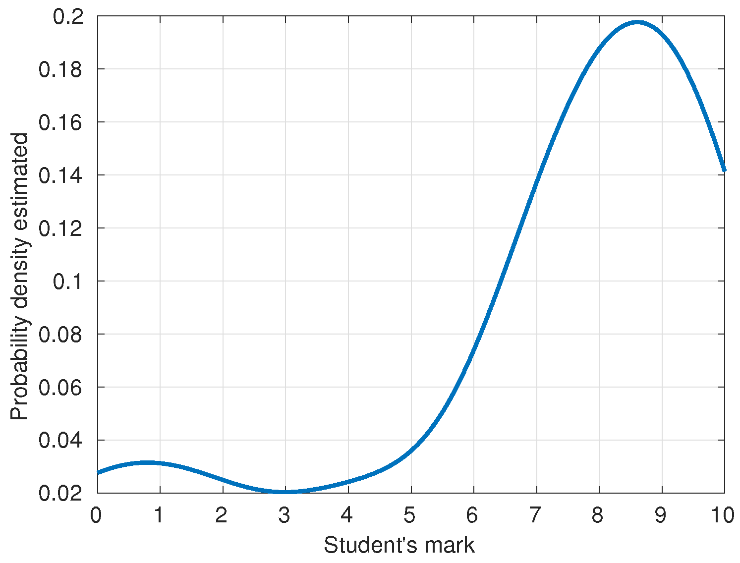
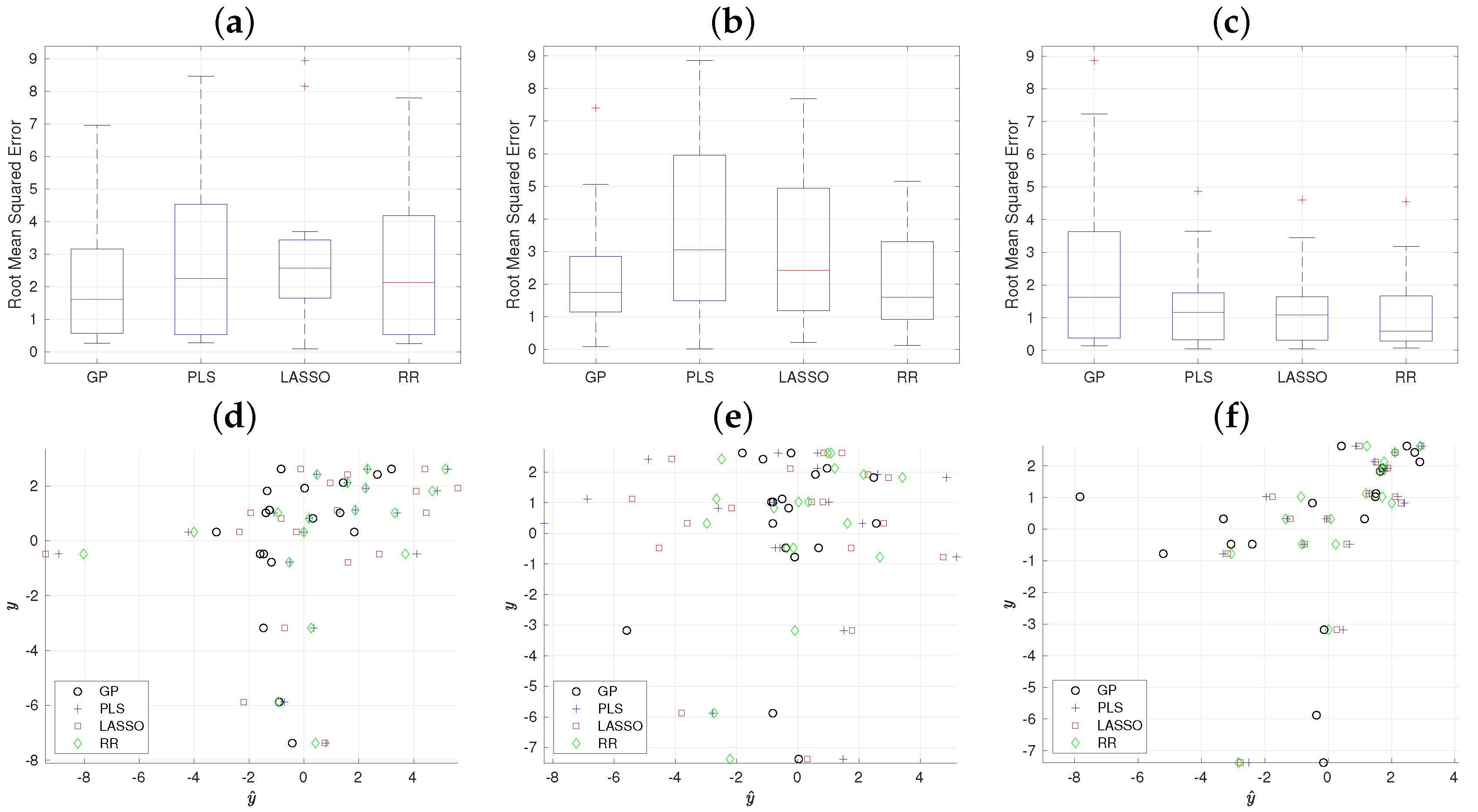
3.3. Student Performance Analysis

This section provides a comprehensive comparison of the various methods and data sets used in the study to evaluate student performance. We evaluate the performance of four machine learning methods: Gaussian Processes (GP), Partial Least Squares (PLS), LASSO, and Ridge Regression (RR). The metrics chosen to measure the accuracy are the Root Mean Squared Error (RMSE), which indicates the averaged error between the estimated student marks $\widehat{y}$ and the true values y according to

$$\mathrm{RMSE}(y,\widehat{y})=\sqrt{\frac{{\sum }_{i=1}^n{(y-\widehat{y})}^2}{n}}.$$

The Coefficient of Variation (CV) is a measure of dispersion of a frequency distribution; in our case, we compute the CV $=\frac{\sigma }{\mu }$ as the quotient between the standard deviation and the mean of the achieved RMSE.

Figure 8 displays the box plots of the proposed methods (GP, PLS, LASSO, and RR) across the three considered data sets. This information is presented in the first row of the figure. The median value of the GP model, denoted with the red line, achieves the best result in all three data sets. The second row of the figure shows the scatter plots of the proposed methods. In order to further evaluate the performance of each method and dataset, the correlation values are presented in

Table 4. Results of the leaving-one-out procedure in terms of performance metrics: Root Mean Squared Error (RMSE) and its standard deviation in brackets (best results are bolded), normalized RMSE (NRMSE), Coefficient of Variation $\mathrm{CV}=\frac{\sigma }{\mu }$, where values of CV $>1$ are in bold, and the Pearson and Spearman Correlation Coefficients with associated p-value in brackets, where best results are in bold and brackets in bold indicate statistical significance.

Metric	Data Source	GP	PLS	LASSO	RR
RMSE	Moodle	2.04 (1.82)	2.76 (2.58)	2.93 (2.30)	2.61 (2.39)
	Socio-Economic	2.26 (1.84)	3.58 (2.98)	3.15 (2.30)	2.10 (1.58)
	Subject marks	2.45 (2.59)	1.38 (1.36)	1.29 (1.28)	1.11 (1.22)
NRMSE	Moodle	0.20 (0.18)	0.28 (0.26)	0.29 (0.23)	0.26 (0.24)
	Socio-Economic	0.23 (0.18)	0.36 (0.30)	0.31 (0.23)	0.21 (0.16)
	Subject marks	0.24 (0.26)	0.14 (0.14)	0.13 (0.13)	0.11 (0.12)
CV	Moodle	0.89	0.93	0.78	0.92
	Socio-Economic	0.81	0.83	0.73	0.75
	Subject marks	1.06	0.99	0.99	1.09
Pearson	Moodle	0.33$(2·{10}^{-1})$	0.25 $(3·{10}^{-1})$	0.30 $(2·{10}^{-1})$	0.30 $(2·{10}^{-1})$
	Socio-Economic	0.24 $(3·{10}^{-1})$	−0.06 $(8·{10}^{-1})$	0.07 $(8·{10}^{-1})$	0.42 $(8·{10}^{-2})$
	Subject marks	0.22 $(4·{10}^{-1})$	0.74 $(5·{10}^{-4})$	0.77 $(2·{10}^{-4})$	0.81 $(5·{10}^{-5})$
Spearman	Moodle	0.50 $(4·{10}^{-2})$	0.54 $(2·{10}^{-2})$	0.45 $(6·{10}^{-2})$	0.57 $(1·{10}^{-2})$
	Socio-Economical	−0.02 $(9·{10}^{-1})$	−0.10 $(7·{10}^{-1})$	−0.01 $(1·{10}^0)$	0.34 $(2·{10}^{-1})$
	Subject marks	0.67 $(2·{10}^{-3})$	0.73 $(5·{10}^{-4})$	0.75 $(4·{10}^{-4})$	0.81 $(5·{10}^{-5})$

.

Table 4 presents various metrics and statistics on the performance of the proposed methods in the student performance task across the three different scenarios: the Moodle LMS data set, the socio-economic survey, and the marks obtained in the mathematics subject. The first row-block displays the Root Mean Squared Error (RMSE) of the different methods, where the best results are shown in bold and belong to the GP and RR methods. It is worth noting that GP is a nonlinear method that can fit the data to more complex relations between inputs and outputs, in our case, between features and marks. Ridge Regression (RR), on the other hand, is a regularised version of the classical least squares, which leads to good results when dealing with multicollinearity relations. In the second row-block, the results achieved for the Normalized RMSE (NRMSE) are shown, where NRMSE $=\frac{\mathrm{RMSE}}{y_{\max }-y_{\min }}.$ This measure provides a percentage interpretation of the result, and the best results, highlighted in bold, were achieved by the GP model and Ridge Regression (RR). The third row-block contains results about the Coefficient of Variation (CV), which is a quotient between the mean and the standard deviation of the errors. It quantifies the ratio of dispersion in the achieved results and expresses the precision and repeatability of an experiment. Typically, a value of CV $>1$ is considered as representing high-valued variance distributions. In our results, in the subject marks data set, values of CV > 1 are marked in bold. Finally, the Pearson correlation coefficient $\rho$ reveals the same conclusions as the RMSE but in a bounded range of $\rho \in [-1,1]$. The best results are presented in bold, and they can be compared with state-of-the-art studies presented in the literature [5,6].

4. Conclusions and Future Work

4.1. Conclusions from the Presented Study

In this study, we have presented a comprehensive comparison of different sources of information on students’ behaviour and its components during a computer science course in the mathematics degree. Student performance is a critical area in education that requires a rich set of relevant features to build specific models that can describe this task. Our study provides a broader comparison of different sources of information commonly employed in the related literature but rarely reviewed together.

We conducted an exhaustive comparison of the data sets using four state-of-the-art machine learning and artificial intelligence methodologies. The inspection of model weights allowed us to gain insights into which features are more relevant to affecting the final student’s marks. The results obtained in the student performance task are comparable with other state-of-the-art methodologies published in the educational area, indicating the effectiveness of the proposed approach.

4.2. Limitations and Future Work

Limitations of our work can be found in the number of years used in the study. In addition, the benefits can be further explored, and more robust conclusions can be obtained from a wider study in terms of the timeline. Also, the present study was centred on a single university, a point which can be further considered to expand in future work.

In future research, one promising direction is to explore the combination of multiple sources of information to build more accurate models that can capture the complex interplay of various factors influencing student performance. This may involve developing novel feature-engineering techniques or adopting more advanced machine learning algorithms to leverage the heterogeneity and complementarity of different data sources. Furthermore, extending the comparative study to include additional courses or educational contexts could help generalise the findings and uncover new patterns and challenges in the prediction of student performance. Such investigations could also contribute to the development of more generalised and transferable models that can be applied to diverse educational settings.

References

1. González, H.B.; Kuenzi, J.J. Science, Technology, Engineering, and Mathematics (STEM) Education: A Primer; Technical Report; Congressional Research Service: Washington, DC, USA, 2012. [Google Scholar]
2. Vo, H.M.; Zhu, C.; Diep, N.A. The effect of blended learning on student performance at course-level in higher education: A meta-analysis. Stud. Educ. Eval. 2017, 53, 17–28. [Google Scholar] [CrossRef]
3. Turnbull, D.; Chugh, R.; Luck, J. Learning Management Systems: An Overview. In Encyclopedia of Education and Information Technologies; Tatnall, A., Ed.; Springer International Publishing: Cham, Switzerland, 2019; pp. 1–7. [Google Scholar] [CrossRef]
4. Van Vaerenbergh, S.; Pérez-Suay, A. Intelligent Learning Management Systems: Overview and Application in Mathematics Education. In Strategy, Policy, Practice, and Governance for AI in Higher Education Institutions; Almaraz-Menéndez, F., Maz-Machado, A., López-Esteban, C., Almaraz-López, C., Eds.; IGI Global: Hershey, PA, USA, 2022; pp. 206–232. [Google Scholar]
5. Bravo-Agapito, J.; Romero, S.J.; Pamplona, S. Early prediction of undergraduate Student’s academic performance in completely online learning: A five-year study. Comput. Hum. Behav. 2021, 115, 106595. [Google Scholar] [CrossRef]
6. Pérez-Suay, A.; Van Vaerenbergh, S.; Diago, P.D.; Pascual-Venteo, A.B.; Ferri, F.J. Data-Driven Modelling through the Moodle Learning Management System: An Empirical Study based on a Mathematics Teaching Subject. IEEE Rev. Iberoam. Tecnol. Aprendiz. 2023, 18, 19–27. [Google Scholar] [CrossRef]
7. Cortez, P.; Silva, A.M.G. Using Data Mining to Predict Secondary School Student Performance. In Proceedings of the 5th Future Business Technology Conference (FUBUTEC 2008), Porto, Portugal, 9–11 April 2008; Brito, A., Teixeira, J., Eds.; pp. 5–12. [Google Scholar]
8. Van Vaerenbergh, S.; Pérez-Suay, A. A Classification of Artificial Intelligence Systems for Mathematics Education. In Mathematics Education in the Age of Artificial Intelligence: How Artificial Intelligence can Serve Mathematical Human Learning; Richard, P.R., Vélez, M.P., Van Vaerenbergh, S., Eds.; Springer International Publishing: Cham, Switzerland, 2022; pp. 89–106. [Google Scholar]
9. Maor, D.; Taylor, P.C. Teacher epistemology and scientific inquiry in computerized classroom environments. J. Res. Sci. Teachnol. 1995, 32, 839–854. [Google Scholar] [CrossRef]
10. Kim, M.C.; Hannafin, M.J.; Bryan, L.A. Technology-enhanced inquiry tools in science education: An emerging pedagogical framework for classroom practice. Sci. Educ. 2007, 91, 1010–1030. [Google Scholar] [CrossRef]
11. Engelbrecht, J.; Harding, A. Teaching Undergraduate Mathematics on the Internet: PART 1: “Technologies and Taxonomy”. Educ. Stud. Math. 2005, 58, 235–252. [Google Scholar] [CrossRef]
12. Balacheff, N.; Kaput, J.J. Computer-Based Learning Environments in Mathematics. In International Handbook of Mathematics Education; Bishop, A.J., Keitel, C., Kilpatrick, J., Laborde, C., Eds.; Kluwer Academic Publishers: Dordrect, The Netherlands, 1996; pp. 469–504. [Google Scholar]
13. Hollebrands, K.; Anderson, R.; Oliver, K. Online Learning in Mathematics Education; Research in Mathematics Education; Springer International Publishing: Cham, Switzerland, 2021. [Google Scholar]
14. Gordon Smith, G.; Ferguson, D. Diagrams and math notation in e-learning: Growing pains of a new generation. Int. J. Math. Educ. Sci. Technol. 2004, 35, 681–695. [Google Scholar] [CrossRef]
15. Bitter, G.G.; Hatfield, M.M. Training Elementary Mathematics Teachers Using Interactive Multimedia. Educ. Stud. Math. 1994, 26, 405. [Google Scholar] [CrossRef]
16. Xingfeng, H.; Huang, R.; Trouche, L. Teachers’ learning from addressing the challenges of online teaching in a time of pandemic: A case in Shanghai. Educ. Stud. Math. 2022, 112, 103–121. [Google Scholar] [CrossRef]
17. Gujarati, D. Multicollinearity: What Happens If the Regressors Are Correlated; Economic Series; McGraw Hill: New York, NY, USA, 2003. [Google Scholar]
18. Vapnik, V.N. The Nature of Statistical Learning Theory; Springer: New York, NY, USA, 1995. [Google Scholar]
19. Hastie, T.; Tibshirani, R.; Friedman, J. The Elements of Statistical Learning; Springer Series in Statistics; Springer: New York, NY, USA, 2001. [Google Scholar]
20. Rasmussen, C.E.; Williams, C.K.I. Gaussian Processes for Machine Learning (Adaptive Computation and Machine Learning); The MIT Press: Cambridge, MA, USA, 2005. [Google Scholar]
21. Schölkopf, B.; Smola, A.J.; Bach, F. Learning with Kernels: Support Vector Machines, Regularization, Optimization, and Beyond; The MIT Press: Cambridge, MA, USA, 2018. [Google Scholar]
22. Garthwaite, P.H. An Interpretation of Partial Least Squares. J. Am. Stat. Assoc. 1994, 89, 122–127. [Google Scholar] [CrossRef]
23. Bishop, C.M. Pattern Recognition and Machine Learning (Information Science and Statistics), 1st ed.; Springer: New York, NY, USA, 2007. [Google Scholar]
24. Tibshirani, R. Regression Shrinkage and Selection via the Lasso. J. R. Stat. Soc. (Ser. B) 1996, 58, 267–288. [Google Scholar] [CrossRef]
25. Bogarín Vega, A.; Romero Morales, C.; Cerezo Menéndez, R. Aplicando minería de datos para descubrir rutas de aprendizaje frecuentes en Moodle. Edmetic 2016, 5, 73–92. [Google Scholar] [CrossRef]
26. Pearson, K. Note on regression and inheritance in the case of two parents. Proc. R. Soc. Lond. 1895, 58, 240–242. [Google Scholar]
27. Spearman, C. The Proof and Measurement of Association between Two Things. Am. J. Psychol. 1987, 100, 441–471. [Google Scholar] [CrossRef] [PubMed]
28. Bunge, M. A General Black Box Theory. Philos. Sci. 1963, 30, 346–358. [Google Scholar] [CrossRef]
29. Molnar, C. Interpretable Machine Learning, 2nd ed.; Lulu Press: Morrisville, NC, USA, 2022. [Google Scholar]
Figure 1. Learning Management System scheme. Adapted from [4] with authors’ permission.
Education 13 00555 g001
Figure 2. Percentage of input variables achieving a value of correlation greater than a threshold value ρ 0 , i.e., | ρ ( x i , x j ) | > ρ 0 , where ρ 0 [ 0 , 1 ] .
Education 13 00555 g002
Figure 3. Kernel density estimate of student marks.
Education 13 00555 g003
Figure 4. Correlations of input variables x i , 1 i n , (a) LMS, (b) socio-economic data, and (c) course marks, with the output variable y (student marks).
Education 13 00555 g004
Figure 5. Stacked feature relevance of the Moodle LMS variables considered in the study. The numbered Event Name Feature (x-axis) are detailed in Table 1.
Education 13 00555 g005
Figure 6. Stacked feature relevance of the socio-economic variables considered in the study. The numbered socio-economic features (x-axis) are detailed in Table 2.
Education 13 00555 g006
Figure 7. Stacked feature relevance of the subject marks considered in the study. The numbered socio-economic features (x-axis) are detailed in Table 3.
Education 13 00555 g007
Figure 8. (ac): box-plots of the four methods used in the experimentation (GP, PLS, LASSO, RR). (df): scatter plot of the true student performance mark y versus the estimated y ^ of each method. The columns represent a data set, the Moodle data, the socio-economic survey, and the subject marks.
Education 13 00555 g008