Introduction to Computational Mathematics Using the Historical Solutions of the “Hundred Fowls” Problem

Abstract

Through programming tasks, the skills and abilities used to solve mathematical problems are developed and improved. In this article we present a programming teaching trajectory using the solutions presented throughout the history of the “hundred fowls” problem. The proposed itinerary is graduated, meaning that it can be used for different educational stages.

1. Introduction

1.1. On Problem Solving

Word problems, especially arithmetic-algebraic ones, occupy a privileged position in mathematics instruction [1,2,3,4]. However, despite the fact that word problems have traditionally been a vehicle for teaching mathematics throughout history, problem solving has not received the same attention in mathematics curricula at different educational levels [5]. In recent decades, problem solving is regaining relevance thanks to different curricular proposals which consider problem solving as an integral part of all mathematical learning and a process standard to be acquired by students [6]. With regard to problem solving in the teaching–learning processes of mathematics, it is usually used in the classroom as a way of practicing what has been learned in the theoretical part or as content in itself [7]. In what follows, we intend to support a methodological proposal based on problem solving as content.

1.2. On the “Hundred Fowls” Problem

In certain cases, the historical study of problems allows for substantiating alternative methodological proposals for the teaching of specific concepts related to mathematics [8]. In this article, we use a number of the solutions shown throughout the history of descriptive problems that are similar to the primitive problem of the “hundred fowls”, which we denote as HF, to design a formative itinerary for teaching computational mathematics.

HF has its origin in China, crosses the East (India and Islam), and finally reaches the medieval West [9]. It appears for the first time in the work of Zhan Qiujian around the fifth century, and has different versions ([8] citing Shen et al., 1999; [9] citing Quian, 1963), one of them being the following:

Problem 1

“A partridge is worth 5 coins; a dove 3 coins; and three sparrows 1 coin. With 100 coins we buy 100 of them. How many partridges, pigeons and sparrows do we have?”

(China, fifth century, cited in Shen et al. [10], 1999, p. 416)

In the compilation of problems by Alcuin of York (775 AD), the problem appears again in the following forms, among others [8]:

Problem 2

“A merchant said: I want to buy 100 pigs for 100 denarii; however, he would pay 10 denarii for a male, 5 for a female, and one for two piglets. Say, whoever knows, how many males, how many females and how many piglets should there be so that none are left over or missing?”

(Alcuin [11], 1863, 804, p. 1145)

Problem 3

“A certain paterfamilias had 20 servants. He ordered that 20 modios of corn be distributed to them in the following way: that the men receive three modios, the women two, and the children half a modius. Say, who can, how many men, how many women and how many children should there be?”

(Alcuin [11], 1863, 804, p. 1154)

Problem 4

“A certain bishop ordered 12 loaves to be distributed among the clergy. He thus provided for each priest to receive two loaves; a half deacon and a reader a quarter. Acting in this way the number of clerics and loaves is the same. Say, who wants, how many priests, deacons and readers should there be?”

(Alcuin [11], 1863, 804, p. 1155)

A more detailed list of versions of the problem of one hundred fowls presented by Alcuin can be found in Table 1 of Martín [9] (2017). Alcuin does not show the resolution procedure in which a possible solution is taken and the values in the equations are substituted to check whether it is correct or not. In addition, it does not offer the various solutions to the problems [9].

In Fibonacci’s work, Liber Abaci, a section of a chapter dedicated to this type of problem appears, where we find problems such as [8]:

Problem 5

A man buys 30 birds that are partridges, pigeons and sparrows, for 30 pence. He buys a partridge for 3 pence, a dove for 2 pence, and 2 sparrows for 1 denarius, that is, 1 sparrow for 1/2 denarius. He asks himself how many birds he buys from each kind.

(Fibonacci [12], 1202, p. 257)

In modern language, the HF problem would be formulated as an indeterminate system of Diophantine equations:

$$\left\{\begin{array}{c}ax+by+dz=p,\hfill \\ x+y+z=q,\hfill \end{array}\right.$$

(1)

where $a,b,d$ are the prices of the birds, p is the total price we have to spend, and q is the number of birds we can buy. In these problems, it is common for the following conditions to be met:

$$\left(C\right)\left\{\begin{array}{c}a,b,p,q,c\in \mathbb{N},\hfill \\ a,b\ge 1,d=\frac{1}{c},c\ge 1,p=q.\hfill \end{array}\right.$$

The solutions are whole numbers greater than 0.

1.3. On Computational Tasks Based on Programming as Problem Solving Tasks

By the end of the twentieth century, easy access to computers offered the opportunity to provide mathematics education with new perspectives for both research and teaching. In addition, the effective use of new emerging technologies in turn allowed for addressing existing knowledge in an improved way, allowing the development of new types of knowledge and mathematical practices [13]. Specifically, and partly thanks to the push of Seymour Papert’s seminal works on constructionism [14], the 1970s and 1980s were marked by strong development of teaching proposals based on programming in computer environments. The objective of these proposals was to facilitate the learning of mathematical concepts and procedures related to problem solving, the use of heuristic strategies, algorithm design, abstraction or logical reasoning.

In the past, these proposals shaped the creation of various programs, aimed at school-level students, such as Logo or Basic (see, among others, [14,15,16,17]). These programs, based on block programming, have today evolved into the well-known Scratch software (https://scratch.mit.edu/, accessed on 11 November 2022). Its ease of use allows it to be used by those without prior programming knowledge. Following these ideas, today we find a multitude of didactic proposals based on this and other similar programs that allow students to start out in computational mathematics by dragging and linking already programmed instructions, like pieces of a puzzle, to create complex programs, games, or interactive simulations (for example, [18,19]).

In all these proposals, in addition to the motivational element offered by technological environments, programming-based computational environments allow new pedagogical objectives that contribute to the development of mathematical thinking in users [20]. Other authors have pointed out that programming tasks favor mathematical reasoning and allow the development of skills and abilities in problem solving [14,17,21,22]. This is mainly due to the similarities between the tasks of writing and designing a program and solving a problem from the point of view of heuristics. Blume and Schoen point out that both activities require [17]:

• Analyzing the problem situation and planning its solution;
• Choosing and applying a resolution strategy;
• Checking and verifying the complete program and the solution.

On the other hand, this paper tries to respond to the recommendations that both teachers’ associations and international organizations have launched on the practical incorporation of technology in the teaching and learning of mathematics [6].

2. Aims

In this article, we present a proposal for the introduction of programming as a possible learning trajectory for problem solving through the history of mathematics, and in particular the historical solutions of the problem of the “Hundred Fowls” presented by Gómez and Martín  [8,9]. More precisely, the aims of this work are:

Aim 1

To design a programming teaching trajectory using the historic solutions of the “Hundred Fowls” problem

Aim 2

To discuss the implementation of the designed pathway with first-year students taking a degree in chemistry

3. Material and Methods

3.1. The Design of the Teaching Trajectory

In order to achieve Aim 1, we design a teaching itinerary to learn computational mathematics based on the classical HF problem and the solutions presented throughout history. To this end, we introduce all the necessary functions or commands showing examples when they are of a higher degree of difficulty. The proposed pathway is divided into sections introducing one or several functions depending on the historical solution presented. For clarity, the complete programming teaching proposal is detailed in Section 4.

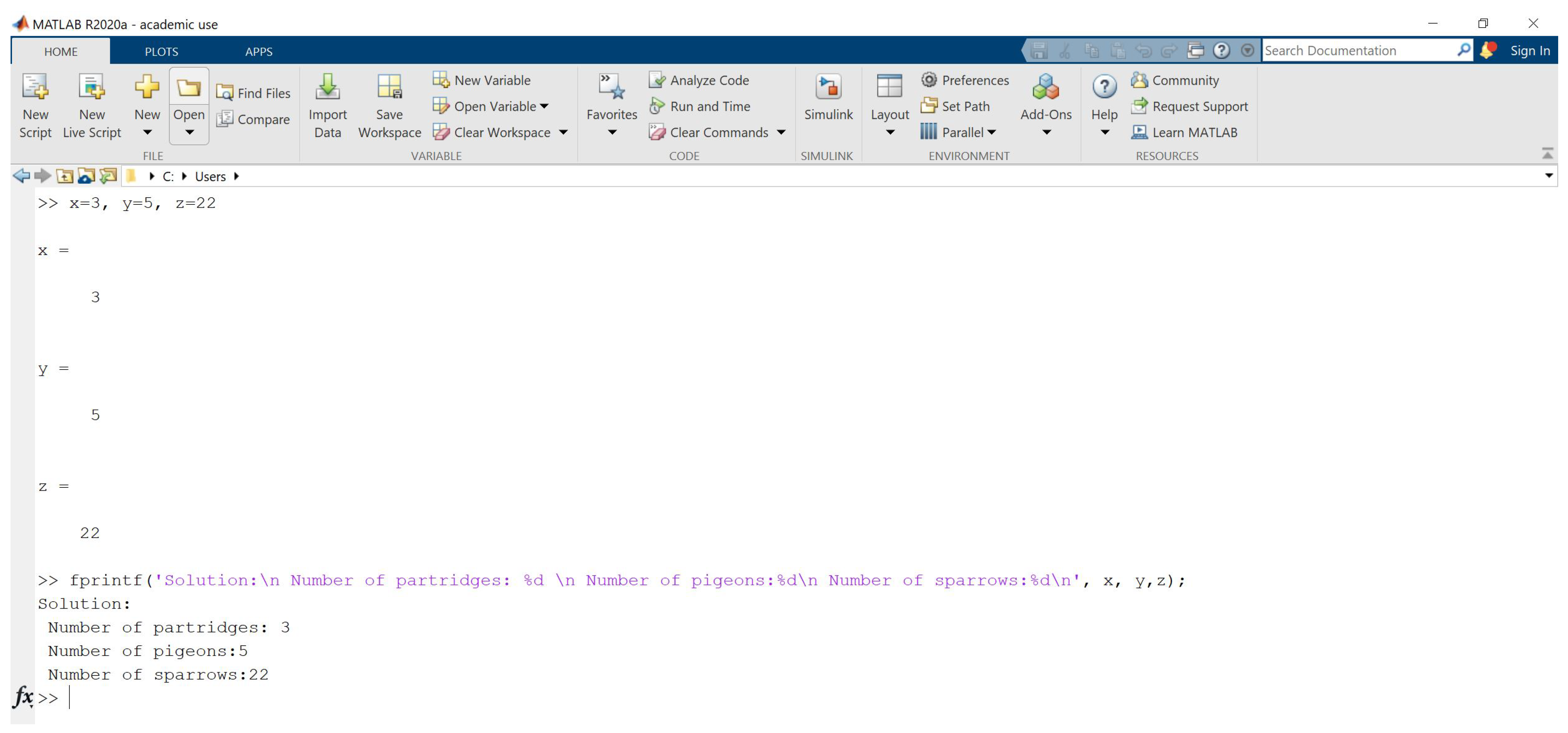
We use Matlab software (https://es.mathworks.com/ (accessed on 11 November 2022), Figure 1), which is a program specially designed for solving mathematical problems from a computational approach. However, the routines can be adapted to other programming languages such as Python, GNU Octave, Scilab, SageMath, etc. They can be seen as pseudocode algorithms.

3.2. The Exploratory Teaching Experiment

Aim 2 is addressed through an exploratory implementation of the designed proposal in an educational context with nearly 180 first-year students taking a degree in chemistry at the University of Valencia in Spain. The experience was configured as a fully online learning intervention previous to the ordinary classes of the course “Numerical Mathematics”, where the following theoretical results were taught: basic statistics, Lagrange interpolation, numerical integration, and numerical solutions of partial differential equations.

Through the material presented in this paper (Section 4) and a set of explanatory online videos, students were instructed on basic programming concepts. The videos can be viewed at the following address: https://www.youtube.com/playlist?list=PLiPJNI1xCP1u_s3i5U_6jnVWKal64jr5R (accessed on 11 November 2022). Thus, this teaching sequence based on the classic HF problem has been used to learn to code the methods seen in theory.

4. The Programming Teaching Trajectory Using the “Hundred Fowls” Problem

4.1. The Data of the Problem: Input and Output Variables

In every program we have a series of input variables (inputs), which in our case is the data we have in the problem, i.e., the price of each of the animals, total price to spend, and number of animals to be purchased if we take into account the conditions (C), that is, the variables $a,b,c$ and p. To enter data, we use the input function. In our particular case, the algorithm is as shown in Algorithm 1.

Algorithm 1: Introduction of input variables

a = input(’Input the price of the partridges\n’);

b = input(’Input the price of the sparrows\n’);

d = input(’Input the price of the pigeons\n’);

p = input(’Input the total number of animals that you want to buy\n’);

The equals symbol (=) in Matlab means assignment; that is, the name of the variable is assigned whatever is written on the screen. The quote symbol (‘…’) means that the phrase appears on the screen, and it is the user who must write the variable. Finally, the \n command means “line break” when the sentence has been typed. If we are interested in knowing the value of $c=1/d$, we introduce that line in our program. When the semicolon symbol is entered at the end of a line, the program does not display the variable. The output variables are the integers $x,y,z$, which represent the number of each type of animal that we can buy with the money. In order to display the results on the screen, we use the following fprintf function that allows us to write the solution to our problem. The use that we make of this is seen in Algorithm 2, although there are many other possibilities, where %d indicates that an integer type variable is displayed, then the name of the variable to be displayed is entered (see Figure 1).

Algorithm 2: Paint variables on the screen
x =	3; y = 5; z = 22;
	fprintf ([’Solution: \n Number of partridges: %d\n’…
	’Number of pigeons: %d\n’…
	’Number of sparrows: %d\n’], …
	x, y, z);

4.2. Programming Qiujian’s Solution with Trial and Error: The if and for Statements

According to [9], Qiujian provides all the possible solutions to the HF problem, though he does not explain in detail a procedure for finding them. We assume that Qiujian solved the problem by trial and error; thus, we program Matlab to carry out this trial and error, trying as far as is possible to make it optimal in terms of operations to be performed by the computer.

To raise the score, we use these two sentences. First of all, the “for” command allows us to give values to a variable. At the end of the instructions, we have to write “end”. Given the complexity of the loops that can be generated with this instruction, we provide the following two simple examples.

Example 1.

Design a program that solves the sum value of the first ten numbers, that is:

$$S=1+2+3+4+5+6+7+8+9+10=\sum _{i=1}^{10}i.$$

First of all, we have to initialize the S variable, which is the variable that stores each of the values. Therefore, we initialize to 0. Subsequently, the variable S is assigned to itself plus i iterating from 1 to 10 (Algorithm 3).

Algorithm 3: Program to calculate the sum of the first 10 numbers
S = 0;	%Initialize the variable S to 0.
for i = 1:10	%(i from 1 to 10)
S = S + i;	%(It assigns to S, the value S+i).
end

In Table 1, we see the value of S in each iteration from Example 1.

Table 1. Value of the sum in each iteration of Example 1.

i	1	2	3	4	5	6	7	8	9	10
S	1	3	6	10	15	21	28	36	45	55

Table 1. Value of the sum in each iteration of Example 1.

i	1	2	3	4	5	6	7	8	9	10
S	1	3	6	10	15	21	28	36	45	55

Example 2.

Design a program that returns the factorial of a number entered by a user (input function); find

$$n!=n(n-1)\dots 1=\prod _{i=1}^{n}i.$$

We have to ask the user to enter a number n, to initialize a variable, and to use the “for” command. Thus, we obtain Algorithm 4.

Algorithm 4: Program to calculate the factorial of a number entered by the user
n = input(’Insert a number \n’);
f = 1;	%Initialize the result, f = 1.
for i = 1:n	%(i from 1 to 10)
f = f ∗ i;
end
f

In Example 2, the value of the factorial number is f. In each iteration, it is multiplied by the value already found and by the next number up to 10.

The second function we work on in this section is If. By means of the if function, we check whether a statement is true or not. As with the for command, end is entered at the end of the statements. This command is used to check an assertion; if it is true, a set of instructions are executed. It is possible to enter other instructions in case the statement is false; however, it is not used in this article. Below, we can see two programs that exemplify their use (Algorithms 5 and 6).

Algorithm 5: Function of the if command
k = 1;	%Initialize k = 1.
p = 1;	%Initialize p = 1.
if p == 1	%It means: if p is equal to 1
k = 2;	%then 2 is inserted in the variable k
end
k

In this case, the result is that the variable k changes, because the statement “p equals 1” is true. In the second example (Algorithm 6), the variable k does not change, as the statement “p is equal to 1” is false.

Algorithm 6: Function of the if command
k = 1;	%Initialize k = 1.
p = 2;	%Initialize p = 1.
if p == 1	%It means: if p is equal to 1
k = 2;	%then 2 is inserted in the variable k
end
k

With these functions, we can program the solution by “trial and error” (Algorithm 7). We analyze the interval where the solutions are contained in order to optimize the program, that is, to perform a smaller number of operations. From the first equation, we have

$$ax+by+dz=p\to ax<p\to 0<x<\frac{p}{a},0<y<\frac{p}{b}.$$

From the second equation, we have

$$x+y+z=p\to z=p-(x+y).$$

Algorithm 7: Program hundredfowls0 to solve the HF problem

a = input(’Input the price of the partridges\n’);

b = input(’Input the price of the sparrows\n’);

d = input(’Input the price of the pigeons\n’);

p = input(’Input the total number of animals that you want to buy\n’);

%x from 1 to p/a

for x = 1:p/a

%y from 1 to p/b

for y = 1:p/b

%We force that z satisfies the second equation.

z = p − (x + y);

%We check the first equation

if (a ∗ x + b ∗ y + d ∗ z == p)

%We show the solutions

fprintf ([’Solution: \n Number of partridges: %d\n’,…

’Number of pigeons: %d\n Number of sparrows:%d\n’],…

x, y, z)

end

end

end

4.3. Programming the Fibonacci Solution: The mod Function

Fibonacci explains the method of solving the problem using the method of alloys:

Divide the 30 pence by the 30 birds; the quotient will be 1 denarius. Say, therefore, I have with 1/2, money with 2 and money with 3, and I want to have money with 1. It is clear that, as in similar problems, the procedure is by the method of alloys, since we have an integer bird’s. Therefore, since the cheapest kind of birds is equal in number to the most expensive kind, say, I have money with 1/2, and money with 2, and money with 3, and wish to have money with 1; that is, I have money with 1, and money with 4, and money with 6, and I want to have money with 2; make the first alloy with the sparrows and partridges and you will get 5 birds for 5 denarii, or 4 sparrows and 1 partridge, and make a second alloy with the sparrows and doves, and you will have 3 birds for 3 de-narii, or 2 sparrows and 1 dove; then in order to have 30 birds in the alloy, put the first alloy three times which will be 12 sparrows and 3 partridges, and there will be 15 birds left to alloy, for which put the second alloy five times, and you will have 10 sparrows and 5 pigeons, and thus, of the previously mentioned 30 birds, there will be 22 sparrows and 5 pigeons and 3 partridges, as shown in the problem.

(Gómez, 2016 citing Fibonacci, 1202, p. 256)

Fibonacci uses the alligation rule; that is, combining the different types of animals, the result is one animal for one denarius. In the first example, he makes an alloy between sparrows and partridges, obtaining four sparrows (at price 1/2) and one partridge (at price 3), for five animals at a price of five pence. The second alloy is then made up of two sparrows (at price 1/2) and one dove (at price 2). If we write the solution offered by Fibonacci in modern mathematical language, we have

$$ax+dz=x+z\to (a-1)x=(1-d)z\to z=\frac{a-1}{1-d}x.$$

If we take $x=1$, $d=1/c$, we have

$$z=\frac{c(a-1)}{c-1}.$$

Therefore, we find that

$$A=c\frac{a-1}{c-1}+1=\frac{ca-1}{c-1}$$

is the number of animals in the first alloy. Similarly, for the second alloy, we have

$$B=\frac{cb-1}{c-1}.$$

In the first example, we find that $A=5$ and $B=3$. To program these two variables, we only have to write the formulas found on the screen.

Finally, we look for how many times the first alloy (denoted as $\overline{x}$) and second alloy ($\overline{y}$) have to appear, making the final result p. In modern parlance, this would be

$$A\overline{x}+B\overline{y}=p\to A\overline{x}=p-B\overline{y}\to \overline{x}=\frac{p-B\overline{y}}{A}.$$

Therefore, it looks for values $(p-B\overline{y})$ that are multiples of A. To program the solution, we can provide values to the variable $\overline{y}$ and check whether they are multiples of A. For that, we use the following mod command, which returns the remainder of the division between two values. The use of this function is direct, that is, if we perform R = mod(8,5), then we are assigning a value of the remainder of 8 divided by 5 to the variable R, which is 3.

With this command along with those previously seen, we can already carry out the program that finds the solutions to the HF problem. First, we analyze the interval where the variable $\overline{y}$ is contained in order to provide it with values. Thus,

$$A\overline{x}=p-B\overline{y}\to 0<p-B\overline{y}\to 0<\overline{y}<\frac{p}{B}=:k.$$

Then, $\overline{y}\in [1,p/B]$. If we have calculated the values A and B, the text of the program is as shown in Algorithm 8.

Algorithm 8: Program to solve the HF problem using the Fibonacci solution

a = input(’Input the price of the partridges\n’);

b = input(’Input the price of the sparrows\n’);

d = input(’Input the price of the pigeons\n’);

p = input(’Input the total number of animals that you want to buy\n’);

c = 1/d;

A = (c∗a-1)/(c-1);

B = (c∗b-1)/(c-1);

k = p/B;

for yb = 1:k         %We start with yb from 1 to p/B

r = mod(p-B∗yb,A);

if r == 0

x = (p-B∗yb)/A;

y = yb;

z = p-(x + y); %We calculate z, using the second equation.

fprintf ([’Solution: \n Number of partridges: %d\n’…

’Number of pigeons:%d\n Number of sparrows: %d\n’],…

x, y, z);

end

end

4.4. Programming the Ventallol Solution

Following the order proposed by Gómez in [8], we can analyze the resolution provided by Ventallol:

A man wants to make a treat and gave his buyer 36 salaries to buy three kinds of fowls, that is, blackbirds, 3 for a salary, chickens, at 2 salaries a piece and capons, at 3 wages the piece; and he wants, that among all there are 36, and that they cost him 36 salaries. I ask, how many will he buy of each lot? He buys the 36 of those that are worth less, that is, shit, and you will find that they cost 12 salaries. Take them out of 36, there are 24 left. See first what a shit is worth and you will find that it is worth 1/3 of salary. Now see how much more a chicken is worth than a piece of shit and you’ll find 1 2/3, put them aside. Then he looks at how much more a capon is worth than a piece of shit, and you will find 2 salaries and 2/3. Now make thirds of everything, that is, of 1 2/3 and they will be 5/3, and likewise of 2 2/3 and they will be 8/3, then you will make 24 thirds of salaries, and they will be 72/3. Now of these 72 make such two parts that one can be divided by 5 and the other by 8 and that there is nothing left in the partition. You will find this like this: remove 5 from 72 as many times, until there is a number that can be divided by 8 exactly, and you will find that it will be 32; and the other will be 40. Divide 32 by 8 and 4 will come; then divide 40 by 5, and 8 will come. And so you see that there will be 4 capons and 8 hens, which are 12, up to 36 there are 24, and there will be so many pieces of shit. And so you will do of all the similar ones.

(Gómez, 2016 citing a Ventallol, 1521/1621, pp. 472–473)

In this case, what Ventallol does is propose a solution by multiplying the second equation by the lower price, which in our case is $1/c$. Thus,

$$\left\{\begin{array}{c}ax+by+\frac{c}{z}=p,\hfill \\ (x+y+z)\frac{1}{c}=\frac{p}{c}.\hfill \end{array}\right.$$

If we subtract, we have

$$\left\{\begin{array}{c}\left(a-\frac{1}{c}\right)x+\left(b-\frac{1}{c}\right)y=\left(1-\frac{1}{c}\right)p,\hfill \\ (ac-1)x+(bc-1)y=(c-1)p.\hfill \end{array}\right.$$

As can be seen in both solutions, Fibonacci’s and Ventallol’s solutions are equivalent; we only have to divide by $c-1$ in the two members of the previous equation. In fact, when calculating x we perform the same calculations, as we can see when $\left(\right(c-1)p-(bc-1\left)y\right)$ is a multiple of $ac-1$. Therefore, the programming is similar (Algorithm 9).

Algorithm 9: Program to solve HF problem using Ventallol’s solution

a = input(’Input the price of the partridges\n’);

b = input(’Input the price of the sparrows\n’);

d = input(’Input the price of the pigeons\n’);

p = input(’Input the total number of animals that you want to buy\n’);

c = 1/d;

A = (c∗a-1);

B = (c∗b-1);

k = (c-1)∗p/(c∗b-1);

for yb = 1:k

r = mod((c-1)∗p-B∗yb,(c∗a-1));

if r == 0

x = ((c-1)∗p-B∗yb)/(c∗a-1);

y = yb;

z = p-(x+y);

fprintf ([’Solution: \n Number of partridges: %d\n’…

’Number of pigeons:%d\n Number of sparrows: %d\n’],…

x, y, z);

end

end

4.5. Diophantine Equations and Their Solutions

Diophantus of Alexandria is considered to be the father of algebra. Little is known about the historical figure. Historians have pointed out that the bishop of Ladoicea, Anatolii, who begins his episcopate in the year 270 BC, dedicates a book on Egyptian computing to his friend Diophantus [23,24]. Therefore, it is known that he lived around the third century BC in Alexandria, and the age at which he died is known thanks to the following riddle dating from the fourth century according to [23], or the fifth or sixth according to [25]:

“God granted him to be a boy for a sixth of his life, and adding to this a twelfth part, He covered his cheeks with hair; He enlightened her with the light of marriage after a seventh part, and five years after their marriage he gave her a son. But alas! Unhappy child born late; after reaching half the measure of his father’s life, cold fate took him away. After consoling his sorrows with the science of numbers for four more years, he ended his life.”

(Boyer, 1986, p. 235 citing Cohen & Drabkin, 1948, p. 27)

If we solve this puzzle, considering x the age at which Diophantus dies, we obtain the following equation:

$$\frac{x}{8}+\frac{x}{12}+\frac{x}{7}+5+\frac{x}{2}+4=x$$

the solution to which is $x=84$. However, we cannot assume this is true either, considering the century in which it is dated [23].

Diophantus’ most important work is the Arithmetica, a compendium of thirteen books, only six of which are preserved. It is a work of great ingenuity and mathematical skill, dedicated especially to the exact resolution of determined and indeterminate equations. The theory that is dedicated to the resolution of indeterminate problems is called Diophantine analysis in modern mathematics and falls under number theory rather than elementary algebra. However, in Arithmetica we find abbreviations and symbols to represent the powers of numbers and the relationships between them [25]. The work of Diophantus is in the second stage of the historical development of algebra, according to Boyer in [25]. This fact justifies his being considered the father of algebra.

Arithmetica consists of a collection of 150 problems, solved with simple numerical examples, where it is intended to show a general method [25]. In these problems, certain equations appear that only admit rational solutions. Especially relevant in the history of mathematics is the first sentence of Problem 8 of Book II, “Divide a given square number into the sum of two squares”, which inspired Fermat to state his famous last theorem:

“On the other hand, it is impossible to separate a cube into two cubes, or a biquadrate into two biquadrates, or generally any power except a square into two powers with the same exponent. I have discovered a truly marvelous proof of this, which however the margin is not large enough to contain”.

(Cohen & Drabkin, 1948 p. 30)

However, we define the diophantine equations as follows:

$$f(x,y)=0,$$

where f is a polynomial with integer coefficients and solutions that are integer values. In particular, we focus in the following equation:

$$Ax+By=P,A,B,P\in \mathbb{Z}.$$

More details on the Diophantine Equations can be found in ([24], Chapter 3).

4.5.1. On the Diophantine Equation $Ax+By=P$

Brahmagupta, the Hindu mathematician of the late sixth century, is known among other contributions for systematizing the arithmetic of negative numbers and zero. In addition, he is credited with discovering a general solution for the linear indeterminate Diophantine equation

$$Ax+By=P,$$

with $A,B,P$ integer numbers different from 0. Brahmagupta knew that if $A,B$ are relatively prime numbers, then the solutions of the equation can be expressed in the following way:

$$x=x_0+tB,y=y_0-tA,$$

with $(x_0,y_0)$ being a particular solution of the equation and t an integer number (Boyer, 1986). Thus, if $A{x}_0+B{y}_0=P$, then

$$A(x_0+tB)+B(y_0-tA)=A{x}_0+B{y}_0+(tAB-tAB)=A{x}_0+B{y}_0=P.$$

This linear equation does not appear in the Diophantus’ work; possibly, he considered it too easy to mention [23].

However, it is not necessary that A and B be relatively prime numbers in order for a solution to exist. This condition can be relaxed, as the linear Diophantine equation has a solution if and only if the greatest common divisor of A and B divides to P, i.e., $gcd(A,B)=d|P$. Indeed, we know (the detailed proof can be found in Burton [23]’s Theorem 2–3, 2007, p. 25) that if $gcd(A,B)=d$, then there exist $x_0$ and $y_0$ integers such that

$$A{x}_0+B{y}_0=d,$$

and from $d|P$ there exists an integer t such that $P=dt$. Thus,

$$(A{x}_0+B{y}_0)t=dt\to A\left(x_{0}t\right)+B\left(y_{0}t\right)=P.$$

On the other hand, if $gcd(A,B)=d$, then there exist $r,s$ such that $A=dr$, $B=ds$. Thus, if there exists a solution to the Diophantine equation, we have

$$P=A{x}_0+B{y}_0=d(r{x}_0+s{y}_0)\to d|P.$$

In fact, we know (from Theorem 2–9 of Burton [23], 2007, p. 40) that the general solution to the equation is provided by

$$x=x_0+t(B/d),y=y_0-t(A/d),t\in \mathbb{Z}.$$

4.5.2. Euclid’s Algorithm as a Solution of the Diophantine Equation $Ax+By=P$

Euclid (325 BC–265 BC), in Book VII, Proposition II of his work The Elements, describes an algorithm for calculating the greatest common divisor by using geometry for the proof of this proposition. We transcribe this proposition and its proof from Euclid’s work using the book [26] in order to make this article self-contained. The proposition is stated as follows: Given two non-prime numbers, find their maximum common measure.

Let AB and CD be two non-prime numbers (for Euclid, these two numbers represent the length of two segments). If CD measures AB (the verb measure is used by Euclid in the same way as the verb divide is used today), then, as CD measures itself, it is common measure to CD and AB, and is therefore the maximum measure. If CD does not measure AB, then by subtracting the smaller number from the larger one successively we can obtain a number EB. In Euclid’s work, it is made explicit that the number EB cannot be the unit, as in the previous proposition it is said that:

Given two unequal numbers and successively subtracting the smaller one from the larger one, if the remaining one never measures the previous one until one unit remains, the initial numbers will be relatively prime numbers.

(Proposition 1. The Elements, Book VII, Euclid; cited in [26])

EB is less than CD; thus, we perform the same process with EB and CD. If EB measures CD, because CD + EB = AB, then EB measures AB, and therefore EB is a common measure. If EB does not measure CD, then another number FD exists such that FD + EB = CD; if FD measures EB, then FD measures FD + EB = CD. If FD measures CD and EB, then FD measures CD + EB = AB, and is therefore a common measure.

Having this common measure, we can now suppose that there exists another measure H which is greater than FD and which measures both AB and CD. If it measures both, then it measures the difference, i.e., H measures AB − CD = EB. If it measures EB and CD, then H measures the difference CD − EB = FD. We have now reached an absurdity, as H is greater than FD and yet divides it.

Let us use an example by assigning numbers to the letters. Thus, we set $AB=10$ and $CD=6$ and calculate its greatest common divisor (which is 2). We start by subtracting $AB-CD=10-6=4=EB$; then, as $EB=4$ does not measure $CD$, we subtract again and obtain

$$CD-EB=6-4=2=FD$$

Now, we measure $EB=4$ with $FD=2$, meaning that $EB=2FD$. As $FD$ measures $EB$, then $FD$ measures $EB+FD$, i.e.,

$$CD=EB+FD=2FD+FD=3FD$$

As $FD$ measures $CD$ and $EB$, then $FD$ measures $CD+EB$:

$$AB=CD+EB=3FD+2FD=5FD$$

Therefore, it is a common measure. Suppose H possesses a value greater than $FD$ that divides $AB$ and $CD$, i.e.,

$$H>FD,H|AB,H|CD,$$

then,

$$H\left|\right(AB-CD)\to H|EB\to H\left|\right(CD-EB)\to H|FD;$$

from $H>FD$ and $H|FD$, we arrive at a contradiction. By means of Euclid’s algorithm in its extended version, a solution to the linear Diophantine equation $Ax+By=P$ can be obtained, provided that (as described in the previous section) the greatest common divisor of A and B divides P. The existence of a solution is provided by Bezout’s Lemma (1730–1783).

Euclid’s extended algorithm consists of obtaining the remainders of the division, clearing them, and inverting the obtained equalities.

We now continue with the example introduced previously; if we have the Diophantine equation $10x+6y=2$, using Euclid’s extended algorithm we obtain

$$\begin{array}{cc}\hfill & 10=6·1+4,\hfill \\ \hfill & 6=4·1+2,\hfill \\ \hfill & 4=2·2+0.\hfill \end{array}$$

Then,

$$2=6-4=6-(10-6)=-10+2·6.$$

As we have seen above, with $x_0=-1$, $y_0=2$, the general solutions is

$$x=x_0+6/2t=-1+3t,y=y_0-10/2t=2-5t,t\in \mathbb{Z}.$$

Let us use another example of the Diophantine equation with $gcd(a,b)=1$. Thus,

$$5x+3y=30.$$

Using Euclid’s extended algorithm, we have

$$\begin{array}{cc}\hfill & 5=3·1+2,\hfill \\ \hfill & 3=2·1+1,\hfill \\ \hfill & 2=2·1.\hfill \end{array}$$

then, $gcd(5,3)=gcd(3,2)=gcd(2,1)=1$. If we apply the algorithm inversely, we obtain

$$1=3-2·1=3-(5-3)=-1·5+2·3.$$

Therefore, $(-30,60)$ is a particular solution of the equation, and the general one is

$$x=-30+3t,y=60-5t,t\in \mathbb{Z}.$$

The only solution with $x,y>0$ is $x=3,y=5$.

4.5.3. Programming a Solution for Diophantine Equations: Functions, Use of Vectors, the while Statement and the abs and ceil Commands

Functions in Matlab are program files that have a series of input and output variables with variables that are internal, that is, they are not modified in the working environment. These are subprograms that execute auxiliary calculations. In our case, we create a function to return the variables of the extended Euclidean algorithm. As input, we have the values A and B, while as output we have the values $gcd(A,B)$ and the particular solution $(x_0,y_0)$, with $y_0\le 0\le x_0$. To perform this function, we analyze the different reminders that we obtain:

$$\begin{array}{cc}\hfill & A=b{q}_1+r_3,\hfill \\ \hfill & B=r_3{q}_2+r_4,\hfill \\ \hfill & r_3=r_4{q}_3+r_5,\hfill \\ \hfill & r_4=r_5{q}_4+r_6,\hfill \\ \hfill & ⋮\hfill \\ \hfill & r_{n-2}=r_{n-1}{q}_{n-2}+r_n,\hfill \\ \hfill & r_{n-1}=r_n{q}_{n-1}+0,\hfill \end{array}$$

where $r_n$ is equal to the greatest common divisor, as we have seen above. We set $r_1=A$ and $r_2=B$ in the i-th step; thus, we have

$$r_{i-2}=r_{i-1}{q}_i+r_i\to r_i=r_{i-2}-r_{i-1}{q}_i.$$

Supposing that

$$\begin{array}{cc}\hfill & r_{i-2}=s_{i-2}A+t_{i-2}B,r_{i-1}=s_{i-1}A+t_{i-1}B\to \hfill \\ \hfill & \to r_i=s_{i-2}A+t_{i-2}B-(s_{i-1}A+t_{i-1}B)q_i=(s_{i-2}-s_{i-1}{q}_i)A+(t_{i-2}-t_{i-1}{q}_i)B,\hfill \end{array}$$

We have

$$\begin{array}{cc}\hfill & s_i=(s_{i-2}-s_{i-1}{q}_i),\hfill \\ \hfill & t_i=(t_{i-2}-t_{i-1}{q}_i).\hfill \end{array}$$

Finally, we determine $s_1,s_2,t_1$ and $t_2$ as follows:

$$\begin{array}{cc}\hfill & A=r_1=s_{1}A+t_{1}B\to s_1=1,t_1=0,\hfill \\ \hfill & B=r_2=s_{2}A+t_{2}B\to s_2=0,t_2=1.\hfill \end{array}$$

Entering a vector in Matlab is similar to assigning a value to a variable, using parentheses with the value of the vector coordinate inside. For example, if we want to introduce $\overrightarrow{v}=(7,-8,5)$, we use the commands in Algorithm 10.

Algorithm 10: Insert the vector $\overrightarrow{v}=(7,-8,5)$ as a Matlab variable

v(1) = 7;   v(2) = −8;  v(3) = 5;

    The while command is used in a similar way to for. As long as the condition is met, the indicated instructions are executed. If the condition is not met, the program exits the while loop. For example, if we want to make a program of the sum of the first ten numbers using while, we write Algorithm 11.

Algorithm 11: Program to add the first 10 numbers using the command while

k = 0; S = 0; %Initialize the variables.

while (k< = 10)

S = S + k;

k = k + 1;

end

S

In a function, the function command is entered, then the output variables; an assignment equals the name of the function and the input variables of the function. If we have initialized all the variables, the function designed in Algorithm 12 is the one corresponding to the Extended Euclidean Algorithm with values A and B.

Algorithm 12: Extended Euclidean algorithm

function [x,y,m]=algeuclext(A,B)

r(1)=A;    %Initialize the vector r

r(2)=B;

s(1)=1;    %Initialize the vector s

t(1)=0;

s(2)=0;

t(2)=1;

i=2;

while (r(i)~=0)

q(i)=floor(r(i-1)/r(i));

r(i+1)=mod(r(i-1),r(i));

s(i+1)=s(i-1)-q(i)∗s(i);

t(i+1)=t(i-1)-q(i)∗t(i);

i=i+1;

end

m=r(i-1); %solution.

x=s(i-1);

y=t(i-1);

In the Euclidean algorithm, we force the solution $x_0$ to always be positive or equal to 0, as all solutions are of the form

$$x_0+tB/d.$$

Because t is an integer, we then take

$$t=d·|x_0|.$$

Thus, if $x_0>0$, then $x_0+B\left|x_0\right|>0$, while if $x_0<0$, then

$$x_0+d\left|x_0\right|B/d=x_0-B{x}_0=x_0(1-B)\ge 0.$$

We only introduce the following lines in our algorithm:

$$\mathrm{y}=\mathrm{y}-\mathrm{abs}\left(\mathrm{x}\right)\ast \mathrm{A};$$

$$\mathrm{x}=\mathrm{x}+\mathrm{abs}\left(\mathrm{x}\right)\ast \mathrm{B};$$

where abs(x) is the function that returns the absolute value of the variable x. It is important that the order of these lines not be altered, because if we modify the variable x then its absolute value (and therefore the variable y) is modified. Note that if $(x_0,y_0)$ is a solution of the Diophantine equation $A{x}_0+B{y}_0=gcd(A,B)$, then if $x_0\ge 0\to y_0\le 0$, as

$$y_0=\frac{1}{B}(gcd(A,B)-A{x}_0).$$

Using Ventallol’s reduction, we obtain

$$(ac-1)x+(bc-1)y=(c-1)p.$$

If we denote as $A=ac-1$, $B=bc-1$, $k=gcd(A,B)$ using Euclid’s extended algorithm, we find a particular solution of the indeterminate equation $Ax+By=k$ called $(x_0,y_0)$; then, this solution multiplied by $(c-1)p/k$ is a solution of the equation, because

$$A\left(x_0\frac{(c-1)p}{k}\right)+B\left(y_0\frac{(c-1)p}{k}\right)=(A{x}_0+B{y}_0)\frac{(c-1)p}{k}=(c-1)p.$$

Therefore, the general solution, as seen in the previous section, is

$$x_0\frac{(c-1)p}{k}-t\frac{B}{k},y_0\frac{(c-1)p}{k}+t\frac{A}{k}.$$

We now only have to determine which values of t result in a plausible solution for the HF problem. To do this, we require that the general solutions be greater than 0. Thus, we have the solution

$$x_0\frac{(c-1)p}{k}\ge 0,y_0\frac{(c-1)p}{k}\le 0\to S_1:=-y_0\frac{(c-1)p}{A}\le t\le x_0\frac{(c-1)p}{B}=:S_2.$$

The last command we use is ceil, which allows us to approximate to the largest integer. As an example, if we use this function, then we have ceil(7.8) = 8, ceil(7.4) = 8. With all these ingredients, we can design Algorithm 13 by introducing the function algeuclext and the values $S_1$ and $S_2$.

Algorithm 13: Algorithm to solve the HF problem from the diophantine equations

a=input(’Input the price of the partridges\n’);

b=input(’Input the price of the sparrows\n’);

d=input(’Input the price of the pigeons\n’);

p=input(’Input the total number of animals that you want to buy\n’);

c=1/d;

A=a∗c-1;

B=b∗c-1;

[x0,y0,k]=algeuclext(A,B); %We use the function showed in Alg. 12

S1=ceil(-(y0∗(c-1)∗p/k)∗k/A);

S2=(x0∗(c-1)∗p/k)∗k/B;

for t=S1:S2

x=(x0∗(c-1)∗p/k)-t∗B/k;

y=(y0∗(c-1)∗p/k)+t∗A/k;

z=p-(x+y);

fprintf ([’Solution: \n Number of partridges: %d\n’…

’Number of pigeons: %d\n’…

’Number of sparrows: %d\n’…

x, y, z);

end

5. Discussion on the Exploratory Teaching Experiment

In this section, we discuss additional details on the attitudes and perceptions of the students derived from the implementation of the instruction sequence described above. It is known that many factors affect online learning, as the literature reports [27,28]. With respect to the teaching format of the designed instruction sequence, the fully online design was well received. Students considered this approach to be practical, as they were allowed to work asynchronously at their own pace. This fact is aligned with the research on learners’ positive attitudes towards online learning [29,30,31]. The literature shows an important learning curve with respect to high-level coding literacy [32,33]. For this reason, the students perceived the material provided, i.e., the videos, exercises, and examples, as being very useful. In particular, they rated it as very profitable to dispose of prior self-study material graded in difficulty.

However, a number of limitations were observed in the implementation of this teaching sequence, the most remarkable of which was that the teaching itinerary did not reduce the differences in coding performance among the implicated students. This fact forced the teachers to revisit basic coding concepts in the first offline sessions of the course. A possible explanation for this fact could be the different commitment levels of the students to work independently in online learning contexts [34,35].

6. Conclusions

In this paper, we have presented and implemented an itinerary based on a classical problem and its solutions shown throughout history as a teaching–learning program to learn computational mathematics. Concerning Aim 1, we designed a teaching trajectory. For each solution, new functions were introduced and the algorithms were optimally established. With respect to Aim 2, we carried out a fully online teaching experiment using the designed trajectory. This exploratory experiment resulted in positive attitudes among the involved students regarding its use in online learning. Through this type of activity, we intend to obtain significant learning itineraries for students, offering a combined introduction to programming, computational mathematics, and the history of mathematics.

References

- Kieran, C. Research on the teaching and learning of algebra. In Handbook of Research on the Psychology of Mathematics Education: Past, Present, and Future; Gutiérrez, Á., Boero, P., Eds.; Sense Publishers: Rotterdam, The Netherlands, 2006; pp. 11–49. [Google Scholar]
- Kieran, C. Algebra Teaching and Learning. In Encyclopedia of Mathematics Education; Lerman, S., Ed.; Springer: Dordrecht, The Netherlands, 2014; pp. 27–32. [Google Scholar]
- Schoenfeld, A.H. Learning to think mathematically: Problem solving, metacognition, and sense making in mathematics. In Handbook of Research on Mathematics Teaching and Learning; Grouws, D.A., Ed.; National Council of Teachers of Mathematics: Reston, VA, USA, 1992; pp. 334–370. [Google Scholar]
- Sutherland, R.; Rojano, T.; Bell, A.; Lins, R. (Eds.) Perspectives on School Algebra; Kluwer Academic Publishers: Dordrecht, The Netherlands, 2002. [Google Scholar]
- Stanic, G.; Kilpatrick, J. Historical perspectives on problem solving in the mathematics curriculum. In The Teaching and Assessing of Mathematical Problem Solving; Charles, R., Silver, E., Eds.; National Council of Teachers of Mathematics: Reston, VA, USA, 1988; pp. 1–22. [Google Scholar]
- National Council of Teachers of Mathematics. Principles and Standards for School Mathematics; NCTM: Reston, VA, USA, 2000. [Google Scholar]
- Puig, L. Elementos de Resolución de Problemas; Comares: Granada, Spain, 1996. [Google Scholar]
- Gómez, B. Problemas descriptivos y pensamiento numérico: El caso de las cien aves de corral. PNA 2016, 10, 218–241. [Google Scholar] [CrossRef]
- Martín, P. El problema de las cien aves: De Alcuino a Fibonacci. SUMA Revista Sobre Enseñanza y Aprendizaje de las Matemáticas 2017, 86, 19–27. [Google Scholar]
- Shen, K.; Crossley, J.N.; Lun, A. The Nine Chapters on the Mathematical Art: Companion and Commentary; Oxford University Press: Oxford, UK, 1999. [Google Scholar]
- Alcuin. Propositiones ad acuendos juvenes. In Patrologiae Cursus Completus: Patrologiae Latinae; Migne, J.P., Ed.; Petit-Montrouge: Paris, France, 1863; pp. 1143–1160. [Google Scholar]
- Fibonacci. Liber Abaci. In A Translation into Modern English of Leonardo Pisano’s Book of Calculation (Original, 1202); Sigler, L., Ed.; Springer: New York, NY, USA, 2002. [Google Scholar]
- Hoyles, C.; Lagrange, J.B. (Eds.) Mathematics Education and Technology-Rethinking the Terrain: The 17th ICMI Study; Springer: New York, NY, USA, 2010. [Google Scholar] [CrossRef]
- Papert, S. Mindstorms: Children, Computers and Powerful Ideas; Basic Books: New York, NY, USA, 1980. [Google Scholar]
- Clements, D.H. Logo and cognition: A theoretical foundation. Comput. Hum. Behav. 1986, 2, 95–110. [Google Scholar] [CrossRef]
- Noss, R. How do children do mathematics with LOGO? J. Comput. Assist. Learn. 1987, 3, 2–12. [Google Scholar] [CrossRef]
- Blume, G.W.; Schoen, H.L. Mathematical Problem-Solving Performance of Eighth-Grade Programmers and Nonprogrammers. J. Res. Math. Educ. 1988, 19, 142–156. [Google Scholar] [CrossRef]
- Dorling, M.; White, D. Scratch: A Way to Logo and Python. In Proceedings of the 46th ACM Technical Symposium on Computer Science Education, Kansas City, MO, USA, 4–7 March 2015; pp. 191–196. [Google Scholar] [CrossRef]
- Sáez, J.M.; Cózar, R. Pensamiento computacional y programación visual por bloques en el aula de Primaria. Educar 2017, 53, 129–146. [Google Scholar] [CrossRef]
- Beatty, R.; Geiger, V. Technology, Communication, and Collaboration: Re-thinking Communities of Inquiry, Learning and Practice. In Mathematics Education and Technology-Rethinking the Terrain: The 17th ICMI Study; Hoyles, C., Lagrange, J.B., Eds.; Springer: New York, NY, USA, 2010; pp. 251–284. [Google Scholar] [CrossRef]
- Chao, P.Y. Exploring students’ computational practice, design and performance of problem-solving through a visual programming environment. Comput. Educ. 2016, 95, 202–215. [Google Scholar] [CrossRef]
- Mannila, L.; Dagiene, V.; Demo, B.; Grgurina, N.; Mirolo, C.; Rolandsson, L.; Settle, A. Computational Thinking in K-9 Education. In Proceedings of the ITiCSE-WGR ’14: Working Group Reports of the 2014 on Innovation & Technology in Computer Science Education Conference, Uppsala, Sweden, 23–25 June 2014; ACM: New York, NY, USA, 2014; pp. 1–29. [Google Scholar] [CrossRef] [Green Version]
- Burton, D.M. Elementary Number Theory, 6th ed.; McGraw-Hill: New York, NY, USA, 2007. [Google Scholar]
- Bashmakova, I.G. Diophantus and Diophantine Equations; Nauka: Moscow, Russia, 1997. [Google Scholar]
- Boyer, C.B. A History of Mathematics; Wiley: Hoboken, NJ, USA, 1968. [Google Scholar]
- Puertas, M.L. Elementos (Libros V-IX); Gredos: Madrid, Spain, 1994. [Google Scholar]
- Ulum, H. The effects of online education on academic success: A meta-analysis study. Educ. Inf. Technol. 2022, 27, 429–450. [Google Scholar] [CrossRef] [PubMed]
- Guo, L. How should reflection be supported in higher education?—A meta-analysis of reflection interventions. Reflective Pract. 2022, 23, 118–146. [Google Scholar] [CrossRef]
- Alomyan, H.; Au, W. Exploration of instructional strategies and individual difference within the context of web-based learning. Int. Educ. J. 2004, 4, 86–91. [Google Scholar]
- Zhang, P.; Bhattacharyya, S. Students’ Views of a Learning Management System: A Longitudinal Qualitative Study. Commun. Assoc. Inf. Syst. 2008, 23, 20. [Google Scholar] [CrossRef]
- Uden, L.; Sulaiman, F.; Lamun, R.F. Factors Influencing Students’ Attitudes and Readiness towards Active Online Learning in Physics. Educ. Sci. 2022, 12, 746. [Google Scholar] [CrossRef]
- Poynton, T.A. Computer literacy across the lifespan: A review with implications for educators. Comput. Hum. Behav. 2005, 21, 861–872. [Google Scholar] [CrossRef]
- Christiansen, H. Teaching computer languages and elementary theory for mixed audiences at university level. Comput. Sci. Educ. 2004, 14, 205–234. [Google Scholar] [CrossRef]
- Hartnett, M. The Importance of Motivation in Online Learning. In Motivation in Online Education; Hartnett, M., Ed.; Springer Singapore: Singapore, 2016; pp. 5–32. [Google Scholar] [CrossRef]
- Kim, K.J.; Frick, T.W. Changes in Student Motivation During Online Learning. J. Educ. Comput. Res. 2011, 44, 1–23. [Google Scholar] [CrossRef] [Green Version]
Figure 1.
Matlab screen after executing the fprintf command.
Disclaimer/Publisher’s Note: The statements, opinions and data contained in all publications are solely those of the individual author(s) and contributor(s) and not of MDPI and/or the editor(s). MDPI and/or the editor(s) disclaim responsibility for any injury to people or property resulting from any ideas, methods, instructions or products referred to in the content. |
© 2022 by the authors. Licensee MDPI, Basel, Switzerland. This article is an open access article distributed under the terms and conditions of the Creative Commons Attribution (CC BY) license (https://creativecommons.org/licenses/by/4.0/).
Share and Cite
MDPI and ACS Style
García-Moreno, M.Á.; Yáñez, D.F.; Diago, P.D. Introduction to Computational Mathematics Using the Historical Solutions of the “Hundred Fowls” Problem. Educ. Sci. 2023, 13, 18. https://doi.org/10.3390/educsci13010018
AMA Style
García-Moreno MÁ, Yáñez DF, Diago PD. Introduction to Computational Mathematics Using the Historical Solutions of the “Hundred Fowls” Problem. Education Sciences. 2023; 13(1):18. https://doi.org/10.3390/educsci13010018
Chicago/Turabian StyleGarcía-Moreno, Miguel Á., Dionisio F. Yáñez, and Pascual D. Diago. 2023. "Introduction to Computational Mathematics Using the Historical Solutions of the “Hundred Fowls” Problem" Education Sciences 13, no. 1: 18. https://doi.org/10.3390/educsci13010018
Note that from the first issue of 2016, this journal uses article numbers instead of page numbers. See further details here.