Which Liquidity Proxy Measures Liquidity Best in Emerging Markets?

Abstract

This study empirically investigates the low-frequency liquidity proxies that best measure liquidity in emerging markets. We carry out a comprehensive analysis using tick data that cover 1183 stocks from 21 emerging markets, while also comparing various low-frequency liquidity proxies with high-frequency spread measures and price impact measures. We find that the Lesmond, Ogden, and Trzcinka (LOT) measure is the most effective spread proxy in most emerging markets. Among the price impact proxies, the Amihud measure is the most effective.

1. Introduction

The importance of liquidity extends far beyond the traditional domain of market microstructure research. There is mounting evidence that liquidity is important in asset pricing. Numerous studies document the pricing of illiquidity, and how it affects stock returns (Amihud and Mendelson 1986; Brennan and Subrahmanyam 1996; Chalmers and Kadlec 1998; Eleswarapu 1997; Amihud 2002), among others. Other studies report that liquidity commonality systematically affects expected returns (Acharya and Pedersen 2005; Pástor and Stambaugh 2003; Sadka 2006). The importance of liquidity is not limited to asset pricing; it is an important factor in corporate finance as well. When the liquidity of a company affects its required return and cost of capital, it has important implications for corporate financial policies. Empirical studies examine how liquidity is linked to capital structure decisions (Lesmond et al. 2008; Lipson and Mortal 2007; Bharath et al. 2009), payout policies (Amihud and Li 2006; Banerjee et al. 2007), information disclosure (Coller and Yohn 1997), and corporate governance (Brockman and Chung 2003).

Most literature on liquidity, including the studies mentioned above, focuses on the markets in the United States (U.S.) or developed markets. However, liquidity may have even greater impacts on emerging markets, as emphasized by Bekaert et al. (2007). Emerging markets are generally characterized by low transparency and limited portfolio choices due to a lack of diversity in available securities (Bekaert et al. 2007). When compared to investors in developed markets, investors in emerging markets tend to be more short-term oriented. Short-term investors are more likely to be concerned about the liquidity of securities. Besides, corporations in emerging markets are characterized by more concentrated ownership than those in developed markets, and they often face severe corporate governance problems. All of these considerations imply that liquidity may have a greater role to play in emerging markets than in developed markets.

While the role of liquidity is instrumental in emerging markets, research on emerging market liquidity is scant at best. This is in contrast to the attention being paid to liquidity in emerging markets lately, due to the dramatic growth of these markets, and the steady global capital market liberalization that has been underway for the past two decades. The primary reason for this lack of research is the paucity of transaction level data on emerging stock markets. To circumvent this problem, some researchers use proxies for liquidity that were obtained from daily return and/or volume data. However, the efficacy of their analysis critically hinges upon the effectiveness of the liquidity proxies that they employ. The most comprehensive study so far regarding the effectiveness of various low-frequency liquidity proxies is by Goyenko et al. (2009).1

The study by Goyenko et al. (2009) considers horse races with more than a dozen low-frequency liquidity proxies. It evaluates the correlation between each of the proxies and various benchmark liquidity measures that were retrieved from high-frequency data on the U.S. markets. The study concludes that many low-frequency liquidity measures perform reasonably well, but also adds a caveat by pointing out that the results may not apply to international markets, particularly emerging markets. Goyenko et al. (2009) state, “We do not know whether the measures are effective on international data, especially in relation to those stocks with extremely thin trading” (p. 180).

Our study takes up the analysis of this statement and evaluates whether some popular low-frequency liquidity proxies capture high-frequency liquidity measures effectively in emerging markets, and if they do, which proxy best measures liquidity.

This study is not the first to analyze the effectiveness of low-frequency liquidity proxies in emerging markets. Lesmond (2005) carries out comprehensive stock level comparisons of low-frequency liquidity proxies in 23 emerging markets. Lesmond’s (2005) high-frequency liquidity benchmark relies on quarterly recorded quoted spreads. The quoted spread recorded at the end of the day (more specifically, the last day of each quarter) may overstate the average spread in the market because of its well-known U-shaped intraday pattern (McInish and Wood 1992). This problem is exacerbated in the case of small firms and infrequently traded stocks, both of which are common attributes of firms in emerging markets. More importantly, the quoted spread reveals only partial information about liquidity. The quoted spread measures the pre-trade transaction costs (i.e., potential transaction costs) but not the post-trade costs (i.e., actual transaction costs). The actual transaction costs that are borne by investors are measured more accurately by the effective spread, and there is no guarantee that a liquidity proxy that measures the quoted spread best would also measure the effective spread most efficiently. Moreover, extant literature on market microstructure breaks up the spread into post-trade price reversal, and adverse price change—the former being pure immediacy costs and the latter being the loss to the informed, or, simply, price impact.

Understanding these two sources of liquidity costs is of particular importance for emerging markets investors. Since many stocks in emerging markets are traded infrequently, the levels of immediacy costs could be multiple times higher than usually observed in developed markets. Investors in emerging markets could also face substantial information costs because of the lack of transparency in the information environment. Knowledge of the effectiveness of various low-frequency liquidity measures as proxies for different aspects of liquidity costs, such as the effective spread, pure immediacy costs, and price impact, offers invaluable information to emerging market investors.

This paper uses unique and comprehensive tick-by-tick data sets on 1183 stocks from 21 emerging stock markets, spanning four continental regions. The data are electronically fed by the Bloomberg Terminals in real time for about three months, and include all quote revisions and transactions at the individual stock level. The comprehensiveness of our data allows us to estimate various intraday measures for transaction costs and the price impact for each trade. We then use these estimates as the benchmarks against which we compare various low-frequency liquidity proxies.

We analyze two groups of benchmark liquidity measures that are calculated using the intraday data. Our classification is motivated by the study of Goyenko et al. (2009). The first group includes spread measures such as effective spread (ES), quoted spread (QS), and realized spread (RS). We call this group the “spread benchmarks.” The second group consists of trade induced price impacts, the lambda coefficient LAMBDA (Hasbrouck 2009), the five-minute price impact IMP (Goyenko et al. 2009), and adverse selection costs ASC (Huang and Stoll 1996). This group is called the “price impact benchmarks.”

The low-frequency liquidity proxies are all calculated using daily data. Specifically, we select three spread proxies, and three price impact proxies that are relatively easy to calculate, and have been widely used in empirical studies.2 The three spread proxies include ROLL (Roll 1984), HASB (Hasbrouck 2009), and LOT (Lesmond et al. 1999), while the three price impact proxies include AMIHUD (Amihud 2002), AMIVEST (Cooper et al. 1985), and PASTOR (Pástor and Stambaugh 2003).

To assess the effectiveness of spread proxies, we compare low-frequency spread proxies with high-frequency spread benchmarks. Similarly, to assess the effectiveness of price impact proxies, we compare low-frequency price impact measures with high-frequency price impact benchmarks. We partition 21 emerging markets into four groups (G1 to G4) that are based on the cross-sectional average of the daily turnover of all the stocks within each country. We implement the analysis for each group individually and sort the values by average daily turnover. We consider three measures to examine the effectiveness of liquidity proxies. First, we measure the absolute difference between the median of the liquidity benchmark value and of liquidity proxy from each group. We interpret a smaller difference as evidence of a more effective proxy. Furthermore, we measure the absolute difference between the liquidity benchmark and liquidity proxy at the individual stock level, and we carry out a variety of Wilcoxon rank-sum tests. Second, we calculate the average cross-sectional correlation between a benchmark and a proxy across individual stocks within each group. Third, using regression, we compute the proxy-induced improvement in the coefficient of determination R². The regression originally includes only popular determinants of liquidity, such as stock price, firm size, country dummies, and industry dummies. Thereafter, we add liquidity proxies one at a time, and see how much the adjusted R² has improved.

When we compare spread benchmarks and spread proxies, all three measures (absolute difference, correlation, and incremental R²) generate meaningful economic interpretation. This is because three spread proxies (ROLL, HASB, and LOT) measure round-trip trading costs as a percentage of stock price in a similar manner, and can be directly compared with three spread benchmarks (ES, QS, and RS). We can also arrive at meaningful economic interpretations of the second and third measures (correlation and incremental R²) when we compare the price impact benchmarks and price impact proxies. The first measure, which is absolute difference, is interpreted with care. For example, LAMBDA captures the sensitivity of return of the signed squared volume. IMP is measured as continuously compounded return. ASC is the percentage change of returns. AMIHUD captures the average ratio of absolute return to the U.S. dollar trading volume. The inverse of AMIVEST is similar to the AMIHUD measure. PASTOR captures the sensitivity of excess return on the lagged signed U.S. dollar trading volume. Therefore, in our empirical analysis of the price impact benchmark and price impact proxies, the correlation and incremental R² measures carry more weight.

In our study, we analyze 21 emerging markets comprising eight stock markets in the Asia Pacific, four in Eastern Europe, six in Latin America, and three in Africa and the Middle East. While many of these markets show similarities in that they have generally low levels of liquidity, lack of transparency, and poor investor protection, they also display substantial dissimilarities in terms of trading rules and systems, legal systems, the degree of market openness, and investor composition. We run cross-sectional regressions to examine what factors influence the effectiveness of the liquidity proxies.

The remaining paper is organized as follows. Section 2 explains various high-frequency liquidity benchmarks and low-frequency liquidity proxies. Section 3 describes the datasets and sample construction, while Section 4 contains the empirical results. Finally, Section 5 concludes the paper.

2. Liquidity Variables

2.1. Liquidity Benchmarks Using High-Frequency Data

2.1.1. Spread Benchmarks

We use three spread benchmarks—the quoted spread (QS), the effective spread (ES), and the realized spread (RS). For easier comparison across different countries, we measure the spread as the percentage of the quote midpoint for all the three spread measures. As discussed in detail below, the three spread measures distinctly represent the different aspects of transaction costs.

The quoted spread at time t is calculated as follows, as the difference between the ask quote and the bid quote at time t, divided by the average of the two quotes.

$$Q{S}_t=(a_t-b_t)/m_i,$$

where $a_t$ and $b_t$ are the posted ask price and bid price, respectively at time t, and $m_t$ is the quote midpoint, or the mean of $a_t$ and $b_t$.

The quoted spread measures the pre-trade transaction costs. Even when the quoted spread provides important information about transaction costs, it is not necessarily translated into actual transaction costs. For example, in a quote driven market, where market makers intervene in the trading process, transactions are frequently made within the bid and ask price. Even in an order driven market where most trades take place either at the ask or bid price, traders who are wary of transaction costs will avoid trading on a wide bid-ask spread, waiting until the spread narrows sufficiently. This implies that the transaction costs that investors actually bear could be different from the quoted spread.

Thus, the actual transaction costs that are borne by investors are measured better using the effective spread. The effective spread is defined as the absolute value of the difference between the transaction price and the midpoint of the quotes prevailing at the time of the transaction, divided by the midpoint quote. The round-trip effective spread conditional on a trade that takes place at time t is:

$$E{S}_t=2D_t(p_t-m_t)/m_t,$$

where $p_t$ is the transaction price at time t, and $D_t$ is an indicator variable that equals one for customer buy orders, and negative one for customer sell orders.

Our third spread benchmark is the realized spread. The realized spread matches the price of a trade with its post-trade true value. More specifically, it is the effective spread net of the price impact of a trade. We calculate the percentage realized spread as:

$$R{S}_t=2D_t(p_t-m_{t+\tau })/m_t,$$

where $m_{t+\tau }$ is the midpoint of the bid and ask quotes recorded $\tau$ minutes after transaction time t. $\tau$ is between 5 and 15 min after the trade. The quote midpoint serves as a proxy for the true economic value of the stock after the trade. This spread measure can be interpreted as compensation to the liquidity providers. In other words, it is the price that the liquidity consumers pay to liquidity providers for their immediacy of consumption.

2.1.2. Price Impact Benchmarks

In this study, we employ three high-frequency price impact measures: Hasbrouck’s (2009) λ coefficient (LAMBDA), Goyenko et al.’s (2009) five-minute price impact (IMP), and Huang and Stoll’s (1996) adverse selection costs (ASC). Hasbrouck (2009) estimates that, while using a regression of returns, the slope of the price function is measured over five-minute time intervals while considering the aggregate signed square root of the dollar volume during the same intervals. It is measured as the coefficient λ in the following regression model:

$$r_n=\lambda \left[{\displaystyle \sum _{t}sign(volum{e}_{t,n})\sqrt{volum{e}_{t,n}}}\right]+{\epsilon }_n,$$

where $r_n$ is the return over the nth five-minute interval, $volum{e}_{t,n}$ is the dollar volume of the tth trade during the nth interval, and $sign(volum{e}_{t,n})$ takes the value +1 if the tth transaction is a buy order, and −1 if it is a sell order.

Our next price impact benchmark is the five-minute price impact that was introduced by Goyenko et al. (2009). This measure captures the permanent price change over a five-minute window subsequent to a trade. It measures the change in quote midpoints from the time of the trade to five minutes after the trade.

$$IM{P}_t=2D_t[\ln (m_{t+5})-\log (m_t)],$$

In the above specification, $m_t$ and $m_{t+5}$ are the quote midpoints at t and five minutes after t, respectively.

Our last price impact benchmark is adverse selection costs, as developed by Huang and Stoll (1996). Huang and Stoll (1996) calculate adverse selection costs by subtracting the realized spread from the effective spread. This measure captures the portion of investors’ transaction costs attributable to the permanent price change, as follows:

$$AS{C}_t=E{S}_t-R{S}_t=2D_t(m_{t+\tau }-m_t)/m_t.$$

2.2. Liquidity Proxies from Low-Frequency Data

2.2.1. Spread Proxies

We choose three spread proxies—Roll’s (1984) spread (ROLL), Hasbrouck’s (2009) Gibbs estimate (HASB), and Lesmond et al.’s (1999) LOT measure. Our choice of the proxies is based on whether the measures are commonly used and are relatively easy to estimate. Roll (1984) develops a spread measure that is based on serial covariance in daily returns. Roll’s spread is defined as:

$$ROLL=\{\begin{array}{ll}2\sqrt{-COV(r_t,r_{t-1})},& \mathrm{if}COV(r_t,r_{t-1})\le 0,\\ 2\sqrt{COV(r_t,r_{t-1})},& \mathrm{if}COV(r_t,r_{t-1})>0,\end{array}$$

where COV denotes covariance, and $r_t$, $r_{t-1}$ are daily returns on day t and t − 1, respectively. In accordance with the study by Lesmond (2005), we calculate the spread separately depending on the sign of the serial covariance. This is to avoid the problem of a negative serial return covariance, resulting in an undefined spread.3

The next proxy we use is a spread estimate that is generated numerically using the Gibbs sampler, a simulation procedure based on the Markov Chain Monte Carlo simulation technique. Hasbrouck (2009) applies the Bayesian Gibbs sampling method to compute the effective costs of trading based on the following variant of Roll’s (1984) model:

$$r_t=c\Delta q_t+{\beta }_m{r}_{mt}+{\mu }_t,$$

where $r_t$ is the change in observed trade prices on day t, $\Delta q_t$ is the change in trade directions from t − 1 to t (i.e., $q_t-q_{t-1}$), and $r_{mt}$ is the market return on t. The last term, ${\mu }_t$, is an innovation in the efficient price m (i.e., $m_t-m_{t-1}$) or the change in the efficient price due to the arrival of new public information. The model has two parameters $c$ and ${\beta }_m$ along with latent data on trade direction indicators $q=\{q_1,\dots ,q_T\}$, and efficient prices $m=\{m_1,\dots ,m_T\}$. We use the programs that are available on Hasbrouck’s website.4 The estimated parameter $c$ is the half spread that is implied by the model. Thus, our spread proxy for the round-trip spread is:

$$HASB=2c.$$

Our third spread proxy is the LOT measure developed by Lesmond et al. (1999). The LOT measure estimates the effective spread while considering the notion that informed trading takes place only on nonzero return days. The idea behind it is simple. A zero return on a day implies that the accumulated value of information generated during the day is not large enough to justify the transaction costs imposed during the day. Lesmond et al. (1999) assume the market model as the return generating process for informed traders. Specifically, $r_t$, the observed return of the firm on day t, and, $r_t^{*}$, the unobserved true return of the firm on the same day, are given below in the framework of a limited dependent variable model:

$$r_t^{*}=\beta \times r_{mt}+{\epsilon }_t,$$

where

$$r_t=\{\begin{array}{ll}{r}_t^{*}-{\alpha }_1,& \mathrm{if} r_t^{*}<{\alpha }_1\\ 0,& \mathrm{if} {\alpha }_1\le r_t^{*}\le {\alpha }_2\\ r_t^{*}-{\alpha }_2,& \mathrm{if} r_t^{*}>{\alpha }_1.\end{array},$$

In the above equation, $r_{mt}$ is the market return on day t. ${\epsilon }_t$ is the random error term representing the public information shock. ${\alpha }_1$ and ${\alpha }_2$ are the sell-side transaction cost and the buy-side transaction cost, respectively. The round-trip transaction cost for informed traders can be calculated as the gap between ${\alpha }_2$ and ${\alpha }_1$, as follows:

$$LOT={\alpha }_2-{\alpha }_1.$$

Given $r_t$ and $r_{mt}$, parameters, including ${\alpha }_1$, ${\alpha }_2$, $\beta$, and $\sigma$ can be estimated by maximizing the following log-likelihood function:

$$\begin{array}{ll}\ln L({\alpha }_1,{\alpha }_2,\beta ,\sigma |r_t,r_{mt})=& {\displaystyle \sum _{region=1}\ln \frac{1}{{(2\pi {\sigma }^2)}^{1/2}}-}{\displaystyle \sum _{region=1}\frac{1}{2{\sigma }^2}{(r_t+{\alpha }_1-\beta \times r_{mt})}^2}+\\ & {\displaystyle \sum _{region=2}\ln \frac{1}{{(2\pi {\sigma }^2)}^{1/2}}-}{\displaystyle \sum _{region=1}\frac{1}{2{\sigma }^2}{(r_t+{\alpha }_2-\beta \times r_{mt})}^2}+\\ & {\displaystyle \sum _{region=0}\ln ({\mathsf{\Phi }}_2-{\mathsf{\Phi }}_1),}\end{array}$$

where 0, 1, and 2 represent the regions where the measured daily return is zero, nonzero negative, and nonzero positive, respectively. $\sigma$ is the standard deviation based on nonzero returns. Lastly, ${\mathsf{\Phi }}_1$ and ${\mathsf{\Phi }}_2$ are the standard normal cumulative distribution functions evaluated at Regions 1 and 2, respectively.5

2.2.2. Price Impact Proxies

For price impacts, we examine three well-known low-frequency proxies, including the Amihud (2002) measure or AMIHUD, the Amivest measure (Cooper et al. 1985) or AMIVEST, and the Pástor and Stambaugh (2003) estimate PASTOR. AMIHUD captures the lack of liquidity by dividing the daily returns by the daily dollar volume. The measure shows the price shock that is triggered by a unit of dollar volume. For a given stock, AMIHUD is calculated as

$$AMIHUD=\frac{1}{T}{\displaystyle \sum _{t=1}^T\frac{\left|r_t\right|}{DollarVolum{e}_t}},$$

where T is the number of days with trading volume and $r_t$ is the return on day t.

AMIVEST compares the daily returns with daily volume measured as the number of shares:

$$AMIVEST=\frac{1}{T}{\displaystyle \sum _{t=1}^T\frac{\left|ShareVolum\right|e_t}{\left|r_t\right|}},$$

where T includes only the days with nonzero returns. The above two measures, even if constructed in a similar manner, differ in several aspects. For example, one uses the dollar volume, while the other uses the share volume. While AMIHUD represents illiquidity, AMIVEST shows liquidity. Besides, AMIHUD does not incorporate the days without trading, which contain important information regarding illiquidity. Although AMIVEST does not suffer from this particular limitation, it is limited in that it does not include information from days with a zero return. We use both proxies, since they complement each other.

Our third price impact proxy is a measure that was developed by Pástor and Stambaugh (2003). This measure is obtained after regression of the daily returns in excess of the daily market index returns on signed daily dollar volume. The Pástor and Stambaugh measure is calculated as the coefficient γ, using the following regression model:

$$r_{t+1}^e=\alpha +\beta \times r_t+\gamma \times Sign(r_t^e)\times Volum{e}_t+{\epsilon }_t,$$

where $r_t$ and $r_t^e$ are a stock’s return and the stock’s excess return net of the market index return on day t, respectively. $Sign(r_t^e)$ is the sign of the excess return. $Volum{e}_t$ is the dollar volume on day t. The value of the coefficient $\gamma$ proxies for the magnitude of the price impact:6

$$PASTOR=\left|\gamma \right|.$$

3. Data and Sample

This section describes the data sources and the construction of the sample that we use in this study. The data are derived from three different sources. We collect intraday trade and quote data from real time data feeds in the Bloomberg Terminals. The tick data contain detailed trade and quote information, including the time of quotes to the nearest second, bid and ask prices, bid and ask sizes, trade price and size in number of shares, as well as the condition codes of the bid and ask quotes. We use various filters to ensure that the trade and quote information that we use is not erroneous or affected by outliers:

(1)

Quotes and transactions are used only if they are recorded during the exchange opening hours, and if the quotes or trades have positive prices and positive shares.

(2)

Only valid quotes and trades are used, where a valid quote or trade is defined, as follows:

(a)

If a quote is not the first quote of the day, its price should be within the range of 50–150% of its previous quote.

(b)

If a trade is not the first trade of the day, its price should be within the range of 50–150% of the price of the trade prior to it.

(3)

To obtain a reliable time series average of the daily average spreads, we impose a condition that there should be at least 20 valid trading days for each stock during the entire investigation window. A valid trading day is a day that has at least one valid quoted spread and one valid effective spread. A valid quoted spread is a spread whose size in currency unit is within 0.2 $\times$ (quote midpoint) and a valid effective spread is an effective spread whose size in currency unit is within 0.2 $\times$ (quote midpoint in effect at the time of the trade).

(4)

For the quoted, effective, and realized spreads, we calculate the daily average spread first (an equal weight average of all spreads, not time weighted), and then calculate the average of these daily spreads over the entire period. For each stock, these average spreads in currency units must be smaller than 10% the time series average of the daily prices during the period.

We also use Standard and Poor’s (S&P) Emerging Markets Database (EMDB) for information on emerging markets. We retrieve stock codes, security type codes, market capitalization, and industry sector classification codes from the database. Furthermore, we screen out sample firms by deleting the stocks that experienced stock splits during our sample period, while using the stock split information available from the EMDB database.

We rely on the Datastream International (DS) data to retrieve daily returns. Even if the DS data provide daily volume information, we use the Bloomberg Terminals tick data as the primary source of information on the daily volume. The reason is as follows. All volume information from the DS data is given in units of 1000 shares. However, a unit of 1000 shares is sometimes too large to accurately capture the daily volumes of many stocks in our sample. This is a result of infrequent trading, wherein only a few hundred shares of these stocks are typically traded per day. The DS data record 0 or 1 in the daily trading volume cells for these firms. This eventually leads to too small a variation in the daily volume to guarantee a reasonable estimation of some of the liquidity proxies that utilize daily volume information.

Initially, we collect the trade and quote information for 2105 firms in 23 countries from the Bloomberg Terminal data feed. However, only 1629 of these firms are covered by the EMDB. Furthermore, many of the 1629 firms whose information is available on both the Bloomberg Terminal and EMDB are not covered by the DS data. Even if they are covered in the DS data, some liquidity benchmarks or proxy variables cannot be estimated for various reasons. In our sample, we discard any firm that is not fully covered by all three databases, or it does not produce all liquidity benchmarks and proxies. Finally, two markets, Russia and Turkey, are excluded, since the number of the surviving firms is too small to carry out a reasonable intra-country analysis. Our final sample consists of 1183 firms from 21 emerging markets.

Among the above countries, China has the largest sample with 222 stocks, followed by South Korea with 145 stocks. Czech Republic has the smallest number of stocks at only seven. The number of stocks in each country is reported in

Table 1. Country-by-Country Summary Statistics. Panel A of Table 1 reports the cross-sectional medians of the spread benchmarks calculated using intraday data, and the spread proxies estimated using daily data. The high-frequency spread benchmarks include the quoted spread QS, effective spread ES, and realized spread RS. The low-frequency spread proxies include ROLL (Roll 1984), HASB (Hasbrouck 2009), and LOT (Lesmond et al. 1999). Panel B of the table reports the cross-sectional medians of price impact benchmarks calculated using intraday data and price impact proxies estimated using daily data. The high-frequency price impact benchmarks include LAMBDA (Hasbrouck 2009), IMP (Goyenko et al. 2009), and ASC (Huang and Stoll 1996). The low-frequency spread proxies include AMIHUD (Amihud 2002), AMIVEST (Cooper et al. 1985), and PASTOR (Pástor and Stambaugh 2003). Panel C of the table reports the cross-sectional median values of firm characteristics (stock price, firm size, turnover, volatility, and investability), and market features (market volatility, legal origin, and trading mechanism). The legal origin takes a value of one if the country’s legal system is based on common laws, and is considered zero otherwise. The trading mechanism takes the value of one for a pure limit-order system, and zero for a dealer or a hybrid system. Panel D of the table reports the minimum tick size, whether tick size varies by stock price, currency code, and average month-end exchange rates during our sample period. The sample covers 1183 firms from 21 emerging markets. The sample period is from February to May 2004.

Panel A: Spread Benchmarks and Spread Proxies
Market			High-Frequency Spread Benchmark			Low-Frequency Spread Proxy
Region	Country	N	QS(%)	ES(%)	RS(%)	ROLL	HASB	LOT
Asia	China	222	0.180	0.177	0.036	1.086	2.239	0.176
	India	101	0.318	0.234	0.103	2.506	2.942	0.001
	Indonesia	43	2.973	1.996	1.036	2.246	3.372	4.075
	South Korea	145	0.301	0.273	0.096	1.539	2.654	0.515
	Malaysia	89	0.929	0.706	0.524	1.324	2.298	1.265
	Philippines	39	2.590	1.760	0.879	1.797	2.995	4.514
	Taiwan	106	0.464	0.463	0.211	1.956	2.841	0.674
	Thailand	57	0.710	0.656	0.262	1.593	2.632	1.030
Eastern Europe	Czech Republic	7	1.672	0.612	0.241	1.526	2.092	0.263
	Greece	63	0.740	0.647	0.238	1.176	2.192	0.554
	Hungary	13	0.916	0.765	0.378	1.691	2.550	0.473
	Poland	26	0.534	0.450	0.229	1.067	2.041	0.602
Latin America	Argentina	12	0.938	0.643	0.141	1.694	1.573	0.527
	Brazil	23	2.471	1.486	0.273	1.830	2.302	0.132
	Chile	35	1.933	1.568	0.583	0.732	1.905	1.333
	Mexico	35	1.053	0.701	0.145	1.076	1.967	0.269
	Peru	18	4.097	2.914	0.591	1.340	2.552	4.297
	Venezuela	11	6.761	4.500	1.211	1.150	3.748	8.635
Others	Egypt	48	2.187	1.479	0.779	1.710	2.535	0.699
	Israel	40	0.429	0.299	0.121	1.068	1.726	0.103
	South Africa	50	0.707	0.560	0.185	1.124	2.062	0.583
Panel B: Price Impact Benchmarks and Price Impact Proxies
Market			High-Frequency Price Impact Benchmark			Low-Frequency Price Impact Proxy
			LAMBDA	IMP	ASC	AMIHUD	AMIVEST	PASTOR
Asia	China	222	1.216	0.140	0.136	0.140	0.017	0.011
	India	101	1.477	0.177	0.119	0.233	0.027	0.007
	Indonesia	43	0.020	1.180	1.159	0.004	1.166	0.000
	South Korea	145	0.073	0.217	0.185	0.000	4.415	0.000
	Malaysia	89	1.984	0.241	0.182	1.639	0.002	0.070
	Philippines	39	0.438	0.968	0.832	4.292	0.001	0.059
	Taiwan	106	0.321	0.237	0.234	0.009	0.310	0.000
	Thailand	57	0.157	0.420	0.394	0.040	0.038	0.004
Eastern Europe	Czech Republic	7	0.458	0.370	0.311	0.093	0.128	0.002
	Greece	63	12.519	0.459	0.358	10.120	0.000	0.813
	Hungary	13	0.789	0.402	0.194	0.097	0.038	0.002
	Poland	26	2.869	0.293	0.226	1.385	0.002	0.045
Latin America	Argentina	12	5.207	0.530	0.503	3.187	0.001	0.145
	Brazil	23	0.046	1.281	0.954	0.253	0.010	0.020
	Chile	35	0.053	0.694	0.564	0.013	1.017	0.000
	Mexico	35	0.807	0.561	0.468	0.146	0.031	0.010
	Peru	18	11.545	1.703	1.712	31.924	0.000	0.893
	Venezuela	11	1.887	2.493	2.293	0.267	0.014	0.007
Others	Egypt	48	4.924	0.534	0.487	7.518	0.000	0.512
	Israel	40	0.140	0.266	0.162	0.366	0.009	0.015
	South Africa	50	0.054	0.382	0.340	0.231	0.030	0.008
Panel C: Firm and Market Characteristics
Market		Stock Price ($)	Firm Size ($ Million)	Turnover	Volatility	Investability	Market Volatility	Legal Origin	Trading Mechanism
Asia	China	0.89	571	0.343	0.018	0.000	1.147	0	1
	India	5.70	719	0.123	0.032	0.490	2.210	1	1
	Indonesia	0.07	166	0.168	0.026	0.000	1.742	0	1
	South Korea	13.63	676	0.663	0.022	0.837	1.690	0	1
	Malaysia	1.04	496	0.101	0.014	0.503	0.890	1	1
	Philippines	0.28	228	0.024	0.018	0.000	1.155	0	1
	Taiwan	0.78	1521	0.840	0.025	0.707	1.951	0	1
	Thailand	0.40	507	0.296	0.023	0.435	1.933	1	1
Eastern Europe	Czech Republic	15.09	2658	0.218	0.019	0.569	1.133	0	0
	Greece	7.46	622	0.142	0.020	0.759	1.079	0	1
	Hungary	18.13	289	0.241	0.015	0.000	1.342	0	0
	Poland	13.94	656	0.147	0.014	0.684	1.124	0	1
Latin America	Argentina	1.18	427	0.048	0.020	0.000	2.561	0	0
	Brazil	0.93	949	0.126	0.023	0.923	2.211	0	0
	Chile	1.90	986	0.047	0.014	0.643	0.634	0	1
	Mexico	1.97	1612	0.110	0.016	0.718	1.184	0	1
	Peru	0.56	181	0.039	0.027	0.000	0.983	0	0
	Venezuela	0.26	189	0.005	0.021	0.000	0.906	0	1
Others	Egypt	2.97	86	0.121	0.022	0.000	0.602	0	1
	Israel	10.58	698	0.243	0.014	0.663	0.904	1	1
	South Africa	3.48	909	0.166	0.014	0.877	1.007	1	1
Panel D: Minimum Tick Size and Foreign Exchange Rates
Market		Minimum Tick in Local Currency		Minimum Tick in US Currency (Cents)		Tick Size Varies by Stock Price		Local Currency	Exchange Rate (Local Currency/USD)
Asia	China	0.01		0.1208		No		CNY	8.28
	India	0.01/0.05		0.0224/0.1120		Yes		INR	44.63
	Indonesia	1		0.0114		Yes		IDR	8768.88
	South Korea	1		0.0858		Yes		KRW	1165.19
	Malaysia	0.005		0.1316		Yes		MYR	3.80
	Philippines	0.0001		0.0002		Yes		PHP	56.10
	Taiwan	0.01		0.0301		Yes		TWD	33.21
	Thailand	0.01		0.0251		Yes		THB	39.79
Eastern Europe	Czech Republic	0.01		0.0377		Yes		CZK	26.50
	Greece	0.001		0.1220		Yes		EUR	0.82
	Hungary	1		0.4852		Yes		HUF	206.12
	Poland	0.01		0.2564		Yes		PLN	3.90
Latin America	Argentina	0.001		0.0345		Yes		ARS	2.90
	Brazil	0.01		0.3367		No		BRL	2.97
	Chile	0.001		0.0002		Yes		CLP	616.77
	Mexico	0.001		0.0089		Yes		MXN	11.26
	Peru	0.001		0.0288		Yes		PEN	3.48
	Venezuela	0.01		0.0004		No		VEF	3067.58
Others	Egypt	0.01		0.1616		No		EGP	6.19
	Israel	0.01		0.2203		Yes		ILS	4.54
	South Africa	1		15.1286		No		ZAR	6.61

. The Bloomberg Terminal tick data cover relatively large and liquid firms. This, along with the availability of information from the other data sources, and our restrictive data screening and sample selection procedure, leads to the composition of our final sample of firms. This composition tends to include more liquid firms than average emerging market firms. Nevertheless, even for these more liquid and representative firms, spreads are, in general, substantially higher when compared to the levels that were observed in developed markets.

Our data spans approximately three months from February to May 2004. However, the data periods for each country do not exactly match. For most countries, the starting date is one of 25, 26, or 27 February, while the ending date is one of 3, 4, or 5 May. The number of trading days ranges from approximately 46 to 51 for most countries.

All variables are measured in terms of U.S. dollars. We obtain exchange rates from Factset. During our sample period from February to May 2004, the changes in exchange rates are small. The maximum and minimum in average monthly exchange rate returns from the 21 emerging markets are 1.97% for the Indian Rupee and −0.44% for the Korean Won, respectively.

Our study focuses on the cross-sectional relation between high-frequency liquidity benchmarks and low-frequency liquidity proxies. Existing studies on the U.S. equity markets demonstrate that the cross-sectional patterns of forecasting errors and the correlation between various liquidity proxies have been stable over time (Chung and Zhang 2014; Abdi and Ranaldo 2017). The results from these two studies clearly indicate that the cross-sectional pattern of the effectiveness of liquidity proxies is time invariant. Therefore, we believe that, despite the limitation in our sample period, our analysis still gives valid and valuable information to researchers and practitioners.

4. Empirical Results

4.1. Spread Benchmarks and Spread Proxies

4.1.1. Spread Benchmarks and Spread Proxies

Panel A of Table 1 presents the median spread benchmarks and median spread proxies for each of the 21 emerging markets in our sample. The reported quoted spread displays rich cross-country variation. For example, Venezuela has the highest median quoted spread at 6.76%, while China has the lowest median quoted spread at 0.18%. In fact, for many countries, the median quoted spreads are substantial, reaching as high as 3%. Meanwhile, not all emerging markets have large transaction costs. There are a number of markets with substantially low spreads. While South Korea has the second largest number of sample stocks, its median quoted spread is only 0.30%. Spreads are generally higher in South America than in other regions.

The median quoted spreads that are shown in Table 1 are significantly smaller than those reported by Lesmond (2005). There are two possible reasons for this substantial difference. First, quoted spreads that are reported in Lesmond’s study are based on daily closing quotes, which could overstate the median quoted spread level during the day. The median quoted spreads in our sample are all complied from intraday quotes. Second, our stringent requirements in the sampling and the data filtering process may exclude many firms with extremely large spreads.

The effective spread also exhibits rich cross-sectional dispersion across markets. As expected, a substantial gap exists between the quoted spread and the effective spread for most countries. Furthermore, the proportion of the effective spread to the quoted spread differs dramatically from country to country. In the case of the Czech Republic, the effective spread is slightly more than one-third, or 37% (0.612%/1.672%) of the quoted spread. China is at the other extreme, with an effective spread to quoted spread ratio of 98% (0.177%/0.180%). The median proportion for the whole sample is 76%, which indicates that, in general, post-trade transaction costs are significantly smaller than pre-trade transaction costs. The realized spread also displays an interesting cross-country distribution. The realized spread is interpreted as the proportion of the effective spread attributable to the cost of immediacy. The proportion of the realized spread in the effective spread also shows large variations, ranging from 11% (0.273%/2.471%) for Brazil to 56% (0.524%/0.929%) for Malaysia.

Panel A of Table 1 also reports the medians of the three low-frequency proxies of the spreads. Among the three proxies, ROLL and HASB display the least amount of cross-country dispersion. Both measures are generally between 1% and 2% for most countries. This is in contrast to the rich cross-country dispersion in the effective spread, in which both measures are intended proxies. The LOT measure displays greater variation. For example, the median LOT measure for Venezuela (8.64) is much larger than the median LOT measure for China (0.18). While the magnitudes of the proxies differ significantly from market to market, they show some consistency in that countries with a larger ROLL measure also have generally larger HASB and LOT measures.

4.1.2. Price Impact Benchmarks and Price Impact Proxies

Now, we turn to the summary statistics for price impact benchmarks and price impact proxies. Panel B of Table 1 shows the medians of both high-frequency benchmarks (LAMBDA, IMP, and ASC) and low-frequency proxies (AMIHUD, 1/AMIVEST, and PASTOR). Rich cross-country dispersion is evident in the price impact benchmarks. IMP and ASC are quite similar in magnitude, while LAMBDA is somewhat different from IMP and ASC. Greece has the largest LAMBDA with a value of 12.52. Venezuela has the largest IMP at 2.49 and the largest ASC at 2.29. The larger the price impact measures, the more illiquid the market is.

With respect to price impact proxies, Peru has the largest AMIHUD at 31.92. A larger value of AMIHUD indicates greater illiquidity. It does not take much volume to move the stock price and generate large returns. On the other hand, AMIVEST measures liquidity. South Korea has the highest AMIVEST at 4.42, and the lowest AMIHUD value at 0.00. This indicates that South Korea is the most liquid market among the 21 countries in our sample. A high PASTOR value indicates illiquidity. Peru has the highest PASTOR value at 0.89. While Pástor and Stambaugh (2003) warn against using their measure for individual stocks, the PASTOR measure is constructed keeping in mind liquidity at the portfolio level.

4.1.3. Firm Characteristics, Market Features, Minimum Tick Size, and Foreign Exchange Rate

Panel C of Table 1 reports the cross-sectional median values of firm characteristics (stock price, firm size, turnover, volatility, and investability), and market features (market volatility, legal origin, and trading mechanism). The legal origin takes a value of one if the country’s legal system is based on common laws or it is zero otherwise. The trading mechanism takes the value one for a pure limit-order system, and zero for a dealer or a hybrid system. Panel D of Table 1 reports the minimum tick size, whether tick size varies by stock price, currency code, and the average month-end exchange rates during our sample period.

4.2. The Best Liquidity Proxies

4.2.1. The Best Spread Proxies

In this section, we examine which liquidity proxies act as the best proxies for liquidity benchmarks. We first partition all countries four groups (G1 to G4) based on the average daily turnover of each country.7 G1, which has the highest turnover, includes China, South Korea, Taiwan, and Thailand. G2 includes Brazil, Hungary, Indonesia, Israel, Mexico, and Poland. G3 includes Argentina, Czech Republic, Egypt, Greece, India, Malaysia, and South Africa. G4, which has the lowest turnover, includes Chile, Peru, Philippines, and Venezuela. The number of stocks in each group are 530, 180, 370, and 103, respectively.

To examine which among ROLL, HASB, and LOT more accurately proxy spread benchmarks (ES, QS, and RS), we calculate a minimum gap measure, which is the smallest absolute difference between the median spread proxy and median spread benchmark.

$$GA{P}_{ROLL}=|Median(ROL{L}_i)-Median(Benchmar{k}_i)|,$$

$$GA{P}_{HASB}=|Median(HAS{B}_i)-Median(Benchmar{k}_i)|,$$

$$GA{P}_{LOT}=|Median(LO{T}_i)-Median(Benchmar{k}_i)|,$$

where the median is calculated using sample stocks in each group, for example, i = 1, 2, …, 530 for the G1 group. The results are reported in Panel A of

Table 2. The Best Spread Proxies and Price Impact Proxies of Countries sorted by Turnover. All countries are partitioned into four groups (G1 to G4) based on the average daily turnover of each country. G1, which has the highest turnover, includes China, South Korea, Taiwan, and Thailand. G2 includes Brazil, Hungary, Indonesia, Israel, Mexico, and Poland. While G3 includes Argentina, Czech Republic, Egypt, Greece, India, Malaysia, and South Africa, G4, which has the lowest turnover, incudes Chile, Peru, Philippines, and Venezuela. Panel A of the table reports the cross-sectional medians of spread benchmarks and spread proxies. Spread benchmarks include QS, ES, and RS. Spread proxies include ROLL, HASB, and LOT. Panel B of the table reports the cross-sectional medians of price impact benchmarks, and price impact proxies. Price impact benchmarks include LAMBDA, IMP, and ASC. Price impact proxies include AMIHUD, the inverse of AMIVEST, and PASTOR. The median spread (price impact) proxy that best approximates the median spread (price impact) benchmark in each group is indicated by **. In Panel A for example, the gap GAP_LOT = |Median (LOT_i) − Median (ES_i)| is smallest in G1. Furthermore, in Panel B, the gap GAP_AMIHUD = |Median (AMIHUD_i) − Median (LAMBDA_i)| is smallest in G1. The sample covers 1183 firms from 21 emerging markets. The sample period is from February to May 2004.

Panel A: Spread Benchmarks and Spread Proxies
Group	ES(%)	ROLL	HASB	LOT
G1	0.274	1.380	2.490	0.396 **
G2	0.760	1.423	2.204	0.454 **
G3	0.599	1.532	2.422	0.522 **
G4	1.909	1.210	2.492 **	3.368
	QS (%)
G1	0.297	1.380	2.490	0.396 **
G2	1.074	0.423 **	2.204	0.454
G3	0.792	1.532	2.422	0.522 **
G4	2.620	1.210	2.492 **	3.368
	RS (%)
G1	0.096	1.380	2.490	0.396 **
G2	0.263	1.423	2.204	0.454 **
G3	0.313	1.532	2.422	0.522 **
G4	0.783	1.210 **	2.492	3.368
Panel B: Price Impact Benchmarks and Price Impact Proxies
Group	LAMBDA	AMIHUD	1/AMIVEST	PASTOR
G1	0.365	0.029 **	0.010	0.002
G2	0.184	0.213 **	0.046	0.007
G3	2.087	1.135 **	0.336	0.054
G4	0.268	0.404	0.225 **	0.008
	IMP
G1	0.191	0.029 **	0.010	0.002
G2	0.560	0.213 **	0.046	0.007
G3	0.277	1.135	0.336 **	0.054
G4	0.955	0.404 **	0.225	0.008
	ASC
G1	0.179	0.029 **	0.010	0.002
G2	0.390	0.213 **	0.046	0.007
G3	0.224	1.135	0.336 **	0.054
G4	0.832	0.404 **	0.225	0.008

under the headings ROLL, HASB, and LOT. For each group, the spread proxy that has the smallest gap is indicated by **. The three proxies exhibit stark differences in their effectiveness. The LOT measure is by far the most effective one, dominating the other two proxies in three out of the four groups when the spread benchmark is ES. Furthermore, LOT dominates the other two proxies in two out of the four groups when the spread benchmark is QS, and in three out of the four groups when the spread benchmark is RS. Thus, it appears that LOT is more effective, particularly in active and liquid markets from Groups G1 to G3.

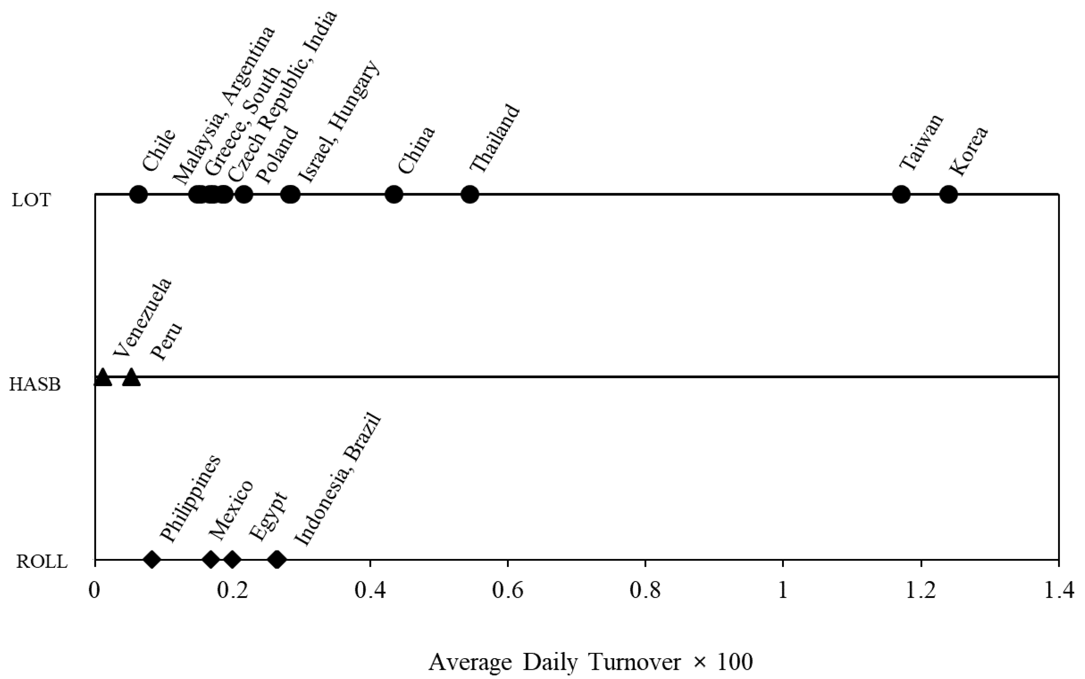
Now, we repeat the analysis and calculate GAP_ROLL, GAP_HASB, and GAP_LOT for each of the 21 emerging markets. Figure 1 plots the dominating proxy against the average daily turnover in each market. If LOT dominates the other proxies in a specific market, then the market is plotted with a circle symbol (●) on the upper parallel line. If ROLL is dominant in a market, then the market is plotted with a triangular delta symbol (▲) on the middle parallel line. If HASB is dominant, then the market is plotted with a diamond symbol (♦) on the bottom parallel line. For example, South Korea, which has a daily turnover of 1.24, the highest among the countries in the sample, and, at the same time, has LOT as the dominating proxy, is plotted as a circle to the far right on the upper parallel line. The pattern in Figure 1 clearly indicates that LOT is the best proxy for effective spread ES in 14 out 21 emerging markets. Our unreported results indicate that LOT is the best proxy for quoted spread QS and realized spread RS in 14 and 16 out of 21 emerging markets, respectively.

Figure 1 also suggests that LOT is more accurate in markets with the highest turnover. For each of the four markets in Group G1, i.e., China, Korea, Taiwan, and Thailand, with the highest turnover, LOT is the dominating proxy for ES. The number of stocks in G1 is 530. This accounts for 45% of the total sample of 1183 stocks. ROLL is the dominating proxy for ES in Venezuela and Peru, while HASB is the dominating proxy for ES in Philippines, Mexico, Egypt, Indonesia, and Brazil.

4.2.2. The Best Price Impact Proxies

To examine which among AMIHUD, 1/AMIVEST, and PASTOR is a more accurate proxy for price impact benchmarks (LAMBDA, IMP, and ASC), we also calculate the following minimum gap measures:

$$GA{P}_{AMIHUD}=|Median(AMIHU{D}_i)-Median(Benchmar{k}_i)|,$$

$$GA{P}_{1/AMIVEST}=|Median(1/AMIVES{T}_i)-Median(Benchmar{k}_i)|,$$

$$GA{P}_{PASTOR}=|Median(PASTO{R}_i)-Median(Benchmar{k}_i)|,$$

where the median is calculated using sample stocks in each group. The results are reported in Panel B of Table 2 under the headings AMIHUD, 1/AMIVEST, and PASTOR. Here, notice that we use the inverse of AMIVEST because this has a positive correlation with AMIHUD. For each group, the price impact proxy that has the smallest gap is indicated by **. The pattern is clear. AMIHUD is by far the most effective measure, dominating the other two proxies in three out of the four groups, when the price impact benchmark is LAMBDA. AMIHUD also dominates the other two proxies in three out of the four groups when the price impact measures are IMP and ASC, respectively.

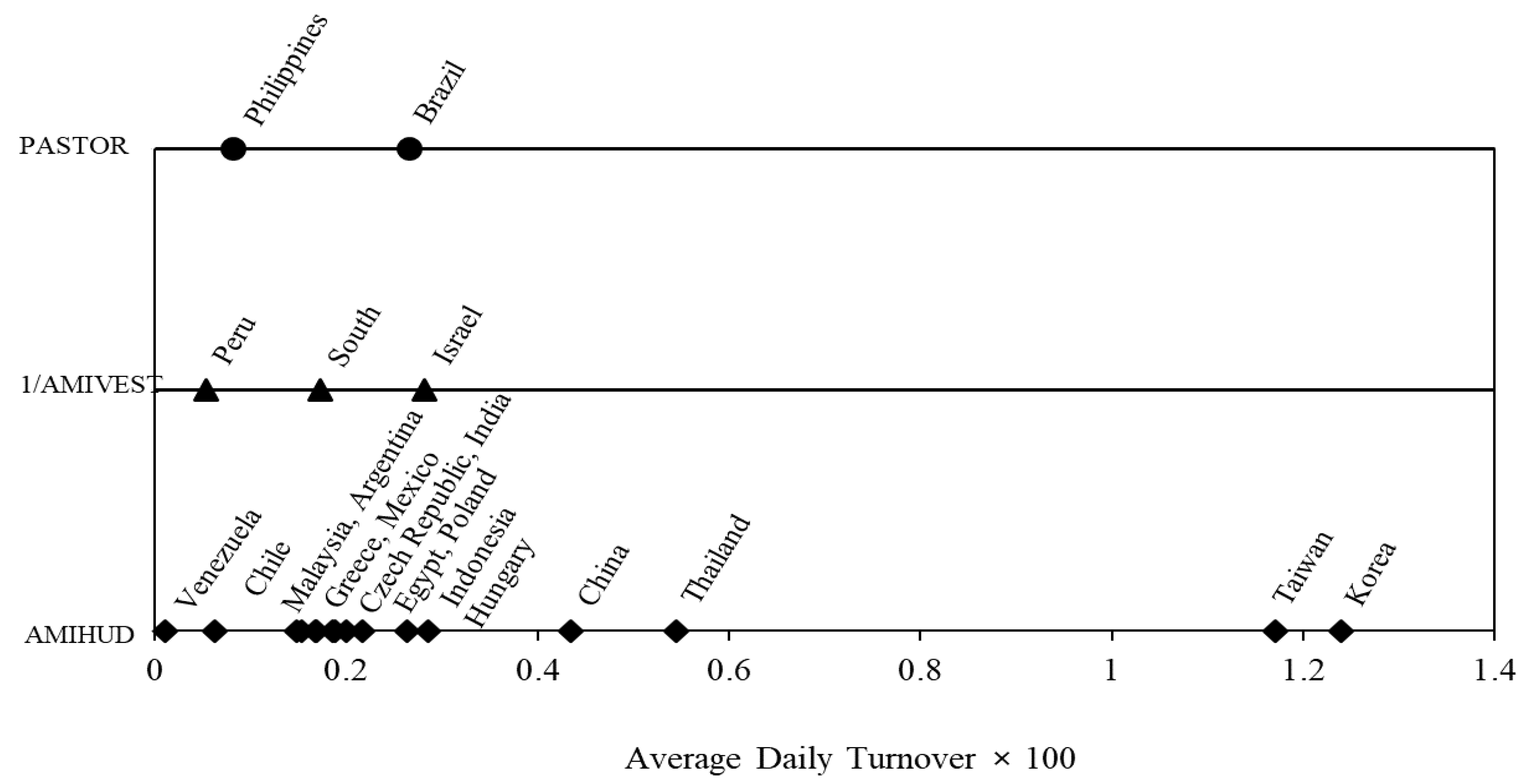
Similarly, we repeat the analysis and calculate GAP_AMIHUD, GAP_1/AMIVEST, and GAP_PASTOR for each of the 21 emerging markets. Figure 2 plots the dominating proxy against the average daily turnover in each market. If PASTOR dominates the other proxies in a specific market, then the market is plotted with a circle symbol (●) on the upper parallel line. If 1/AMIVEST is dominant in a market, then the market is plotted with a triangular delta (▲) on the middle parallel line. If AMIHUD is dominant, then the market is plotted with a diamond symbol (♦) on the bottom parallel line. For example, South Korea, which has a daily turnover of 1.24, the highest among the countries in the sample, and, at the same time, has AMIHUD as the dominating proxy, is plotted with a circle to the far right on the lower parallel line. The pattern in Figure 2 clearly indicates that AMIHUD is the best proxy for the price impact benchmark LAMBDA in 16 out 21 emerging markets. Our unreported results indicate that AMIHUD is the best proxy for IMP and ASC in 14 and 12 out of 21 emerging markets, respectively.

Figure 2 also suggests that AMIHUD is more accurate in markets with the highest turnover. For each of the four markets in Group G1, i.e., China, Korea, Taiwan, and Thailand, with the highest turnover, AMIHUD is the dominating proxy for LAMBDA.

4.3. Wilcoxon Rank-Sum Tests for the Effectiveness of Liquidity Proxies

4.3.1. Effectiveness of Spread Proxies

An analysis of the accuracy of the spread proxies in Figure 1 and Figure 2 is descriptive, without any formal statistical test. To see whether the pattern that is described above is statistically discernible, we calculate the absolute difference (MERR) between the spread proxies (ROLL, HASB, and LOT), and spread benchmarks (ES, QS, and RS) for each stock i, as follows:

$$MER{R}_{ROLL,i}=|ROL{L}_i-Benchmar{k}_i|,$$

$$MER{R}_{HASB,i}=|HAS{B}_i-Benchmar{k}_i|,$$

$$MER{R}_{LOT,i}=|LO{T}_i-Benchmar{k}_i|.$$

MERR is similar to the GAP measure introduced earlier except that, for each group from G1 to G4, GAP calculates the difference in cross-sectional medians between a spread proxy and a spread benchmark, while MERR calculates the difference for each individual stock.

Panel A of

Table 3. Measurement Errors of Spread Proxies and Price Impact Proxies of Countries sorted by Turnover. All countries are partitioned into four groups (G1 to G4) based on the average daily turnover of each country. Panel A of the table reports the median values of the measurement error (MERR) between the spread benchmarks (ES, QS, and RS), and spread proxies (ROLL, HASB, and LOT), respectively. For example, MERR_ROLL,i = |ROLL_i − ES_i|. Panel A then implements the Wilcoxon rank-sum tests for equality between (i) the median |ROLL_i − ES_i| and median |LOT_i − ES_i|, and (ii) the median |HASB_i − ES_i| and median |LOT_i − ES_i|. The significance levels are assigned to the |ROLL_i − ES_i| and |HASB_i − ES_i| columns, respectively. Panel B reports the measurement error between the price impact benchmarks (LAMBDA, IMP, and ASC), and price impact proxies (AMIHUD, 1/AMIVEST, and PASTOR), respectively. For example, MERR_AMIHUD,i = |AMIHUD_i − LAMBDA_i|. Panel B also implements the Wilcoxon rank-sum tests for equality between (i) the median |AMIHUD_i − LAMBDA_i| and median |1/AMIVEST_i − LAMBDA_i|, and (ii) the median |AMIHUD_i − LAMBDA_i| and median |PASTOR_i – LAMBDA_i|. The significance levels are assigned to the |1/AMIVEST_i − LAMBDA_i| and |PASTOR_i − LAMBDA_i| columns, respectively. The sample covers 1183 firms from 21 emerging markets. The sample period is from February to May 2004. *, **, and *** represent statistical significance at 10%, 5%, and 1%, respectively.

Panel A: Spread Proxies
Group	Median Measurement Error
	|ROLLi − ESi|	|HASBi − ESi|	|LOTi − ESi|
G1	1.029 ***	2.193 ***	0.181
G2	0.811 ***	1.316 ***	0.464
G3	0.877 ***	1.673 ***	0.300
G4	1.008 **	1.195 ***	1.604
	|ROLLi − QSi|	|HASBi − QSi|	|LOTi − QSi|
G1	1.003 ***	2.165 ***	0.181
G2	0.892 *	1.162 ***	0.656
G3	0.752 ***	1.545 ***	0.399
G4	1.760	1.199	1.442
	|ROLLi − RSi|	|HASBi − RSi|	|LOTi − RSi|
G1	1.273 ***	2.388 ***	0.290
G2	1.066 ***	1.839 ***	0.256
G3	1.149 ***	1.997 ***	0.328
G4	0.921 ***	1.793 **	2.398
Panel B: Price Impact Proxies
Group	Median Measurement Error
	|AMIHUDi − LAMBDAi|	|1/AMIVESTi − LAMBDAi|	|PASTORi − LAMBDAi|
G1	0.326	0.360	0.366
G2	0.355	0.188 *	0.145 *
G3	1.515	1.645	2.028
G4	0.957	0.740	0.682
	|AMIHUDi − IMPi|	|1/AMIVESTi − IMPi|	|PASTORi − IMPi|
G1	0.184	0.171	0.185 **
G2	0.598	0.522	0.524
G3	0.847	0.265 ***	0.230 ***
G4	1.902	0.953	0.928 ***
	|AMIHUDi − ASCi|	|1/AMIVESTi − ASCi|	|PASTORi − ASCi|
G1	0.170	0.156	0.171 *
G2	0.546	0.423 **	0.372 ***
G3	0.878	0.265 ***	0.183 ***
G4	1.702	0.874	0.784 ***

displays the median MERR for each stock group partitioned by turnover. The results are generally consistent with those that are displayed in Panel A of Table 2 and Figure 1. LOT is the most accurate proxy for ES, QS, and RS. For example, in the top section of Panel A where the spread benchmark is ES, and the turnover is the highest (G1), the median |LOT_i − ES_i| is 0.181%. The median |ROLL_i − ES_i|, and |HASB_i − ES_i| are 1.029% and 2.193%, respectively. We implement the Wilcoxon rank-sum test to see if the median |ROLL_i − ES_i|, and the median |LOT_i − ES_i| are statistically different. The result indicates that the difference between 1.029% and 0.181% is highly significant. A significance level of *** is assigned to the corresponding number corresponding number in the |ROLL_i − ES_i| column. The median |HASB_i − ES_i| of 2.193% and the median |LOT_i − ES_i| of 0.181% are also statistically different. A significance level of *** is assigned to the corresponding number in the |HASB_i − ES_i| column.

4.3.2. Effectiveness of Price Impact Proxies

Now, we calculate the absolute difference (MERR) between the price impact proxies (AMIHUD, 1/AMIVEST, and PASTOR), and price impact benchmarks (LAMBDA, IMP, and ASC) for each stock i, as follows:

$$MER{R}_{AMIHUD,i}=|AMIHU{D}_i-Benchmar{k}_i|,$$

$$MER{R}_{1/AMIVEST,i}=|1/AMIVES{T}_i-Benchmar{k}_i|,$$

$$MER{R}_{PASTOR,i}=|PASTO{R}_i-Benchmar{k}_i|.$$

Panel B of Table 3 displays the median MERR for each stock group partitioned by turnover. The results are notably different from those displayed in Panel B of Table 2 and Figure 2, wherein AMIHUD is the dominating proxy for the price impact benchmarks LAMBDA, IMP, and ASC. When we examine the effectiveness of the price impact proxies at the individual stock level, there is no clear winner, when the price impact benchmark is LAMBDA in the top section of Panel B. However, there is some evidence that when the price impact benchmark is either IMP or ASC, PASTOR turns out to be the winner for less liquid markets in G3 and G4. We conjecture that the results might be driven by larger dispersion in price impact proxy measures, as compared to the results for spread proxy measures. We examine this issue further when we analyze the correlation structure and conduct regression analysis.

4.4. Correlation Analysis

In this section, we examine the cross-sectional correlations between the spread benchmarks and the spread proxies. The correlation is calculated across firms in each country group for each pair of spread benchmark and spread proxy. The correlations with both a predicted sign and statistical significance at the 5% level are indicated with **. In addition, if the correlation is greater than 0.50, it is further indicated with a bold color. We consider that, even if somewhat arbitrary, a correlation of 0.50 or greater is a good indication that the proxy captures the benchmark reasonably well.

Panel A of

Table 4. Cross-Sectional Correlations between Liquidity Benchmarks and Liquidity Proxies. All countries are partitioned into four groups (G1 to G4) based on the average daily turnover of each country. Panel A of the table reports the Spearman cross-sectional correlations between spread benchmarks (ES, QS, and RS), and spread proxies (ROLL, HASB, and LOT). Panel B reports the Spearman cross-sectional correlations between price impact benchmarks (LAMBDA, IMP, and ASC), and price impact proxies (AMIHUD, 1/AMIVEST, and PASTOR). Among the spread proxies that have a significant correlation, the ones larger than 0.50 are in bold. The sample covers 1183 firms from 21 emerging markets. The sample period is from February to May 2004. ** indicates statistical significance at the 5% level.

Panel A: Correlation between Spread and Spread Proxies
	Spread		Spread Proxy
	Benchmark	ROLL	HASB	LOT
G1	ES	0.274 **	0.255 **	0.582 **
	QS	0.265 **	0.246 **	0.575 **
	RS	0.210 **	0.118 **	0.544 **
G2	ES	0.351 **	0.609 **	0.622 **
	QS	0.311 **	0.578 **	0.576 **
	RS	0.260 **	0.503 **	0.691 **
G3	ES	−0.081	0.062	0.636 **
	QS	−0.077	0.054	0.551 **
	RS	−0.084	0.055	0.620 **
G4	ES	0.261 **	0.449 **	0.818 **
	QS	0.258 **	0.438 **	0.802 **
	RS	0.060	0.211 **	0.457 **
Panel B: Correlation between Price Impact and Price Impact Proxies
	Price Impact		Price Impact Proxy
	Benchmark	AMIHUD	1/AMIVEST	PASTOR
G1	LAMBDA	0.800 **	0.787 **	0.713 **
	IMP	−0.113	−0.115	−0.168 **
	ASC	−0.079	−0.080	−0.137 **
G2	LAMBDA	0.606 **	0.633 **	0.550 **
	IMP	0.069	0.006	−0.026
	ASC	−0.049	−0.090	−0.098
G3	LAMBDA	0.715 **	0.759 **	0.716 **
	IMP	0.705 **	0.613 **	0.583 **
	ASC	0.636 **	0.563 **	0.534 **
G4	LAMBDA	0.487 **	0.490 **	0.504 **
	IMP	0.510 **	0.475 **	0.467 **
	ASC	0.534 **	0.502 **	0.498 **

reports the pairwise correlation between the spread proxies (ROLL, HASB, and LOT), and the spread benchmarks (ES, QS, and RS) for each stock group from G1 to G4. It is clear that LOT dominates both ROLL and HASB. The correlation between ROLL and the spread benchmarks are in general between 0.20 and 0.40. The same conclusion can be drawn for HASB, except in Group G2.8 The correlation between LOT and the spread benchmarks are much higher. In general, the correlations are between 0.50 and 0.80 for all four stock groups from G1 to G4. In the unreported results, we repeat the correlation analysis on a country-by-country basis. Overall, the results confirm that the LOT measure tends to do better than either ROLL or HASB. The evidence from the correlation structure is consistent with that based on measurement error at the individual stock level from Panel A of Table 3.

Panel B of Table 4 presents the pairwise correlations between price impact proxies (AMIHUD, 1/AMIVEST, and PASTOR), and price impact benchmarks (LAMBDA, IMP, and ASC). Two clear patterns emerge. First, there is no clear winner among the three price impact proxies when we examine their correlations with price impact benchmarks. Therefore, evidence from the correlation structure confirms the evidence from the measurement error in Panel B of Table 3, regarding the effectiveness of price impact proxies. Second, in the more liquid markets of Groups G1 and G2, the correlation between the price impact proxies and LAMBDA is much higher than the correlation between price impact proxies and either IMP or ASC. Third, the performance of PASTOR is as good as either AMIHUD or 1/AMIVEST. This result is in contrast to the findings by Hasbrouck (2009) and Goyenko et al. (2009), although these two studies draw their conclusions from the U.S. market.

4.5. Incremental Regression R²

4.5.1. The Determinants of Spread Benchmarks

The correlation analysis offers some interesting results. However, these results alone may not fully reveal how much variation in a liquidity benchmark is captured by a variation in a liquidity proxy. This is because a covariate variable can affect both the benchmark and the proxy, spuriously increasing or decreasing the correlation. One needs to control for covariate variables while examining the associations between liquidity benchmarks and liquidity proxies.

One variable is known to affect measured liquidity is price. Another variable is firm size. We include both the log of stock price (PRICE) and the log of firm size (SIZE) as control variables in a cross-sectional regression framework. The dependent variable is one of the high-frequency liquidity benchmarks, while the independent variables are the control variables and a low-frequency liquidity proxy, added one at a time. We run the regressions using all sample stocks. Specifically, the regression takes the following form:

$$SPREA{D}_i={\phi }_0+{\phi }_{1}PRIC{E}_i+{\phi }_{2}SIZ{E}_i+{\displaystyle \sum CDUMs}+{\displaystyle \sum IDUMs+}{\epsilon }_i,$$

(1)

where SPREAD = QS, ES, and RS, respectively. Subscript i refers to individual stocks, i = 1, ..., 1183. Country dummies and industry dummies are included. We obtain the adjusted R², $R_{ADJ1}^2$ from the above regressions. Subsequently, we run the following regressions, adding spread proxies:

$$\begin{array}{cc}\hfill SPREA{D}_i={\phi }_0& +{\phi }_1\log {(PRICE)}_i+{\phi }_2\log {(SIZE)}_i+{\phi }_{3}SPREAD\_PROX{Y}_i\hfill \\ & +{\displaystyle \sum CDUMs}+{\displaystyle \sum IDUMs+}{\epsilon }_i,\hfill \end{array}$$

(2)

where SPREAD_PROXY = ROLL, HASB, and LOT, respectively. The corresponding adjusted R² is $R_{ADJ2}^2$. The incremental adjusted R² is calculated as:

$$Incremental{R}^2=R_{ADJ2}^2-R_{ADJ1}^2.$$

(3)

Panel A of

Table 5. Incremental Regression R²s. Panel A of the table examines the incremental explanatory power of spread proxies in predicting spread benchmarks, after controlling for stock price and firm size. In the first regression, the dependent variable is one of the spread benchmarks (ES, QS, and RS), while the independent variables are the control variables, namely the stock price (PRICE) and firm size (SIZE). The corresponding adjusted R² is $R_{ADJ1}^2$. In the second regression, the dependent variable is one of the spread benchmarks (ES, QS, and RS), while the independent variables are the control variables, stock price and firm size in addition to one of the spread proxies (ROLL, HASB, and LOT). The corresponding adjusted R² is $R_{ADJ2}^2$. The incremental adjusted R² is calculated as: $R_{ADJ2}^2-R_{ADJ1}^2$. Panel B examines the incremental explanatory power of price impact proxies (AMIHUD, 1/AMIVEST, and PASTOR) in predicting price impact benchmarks (LAMBDA, IMP, and ASC). The sample covers 1183 firms from 21 emerging markets. The sample period is from February to May 2004. The t-statistics are in parenthesis. *, **, and *** represent statistical significance at 10%, 5%, and 1% levels, respectively.

Panel A: The Incremental Explanatory Power of Spread Proxies
	Intercept	PRICE	SIZE	ROLL	HASB	LOT	Adjusted R2	Incremental R2
ES	5.956 ***	0.009	−0.306 ***				0.325
	(10.23)	(0.22)	(−6.48)
	5.345 ***	0.022	−0.252 ***	0.296 ***			0.361	0.036
	(8.97)	(0.57)	(−7.17)	(3.84)
	4.879 ***	0.023	−0.265 ***		0.256 ***		0.343	0.018
	(8.45)	(0.53)	(−5.66)		(4.73)
	3.699 ***	−0.001	−0.175 ***			0.122 ***	0.464	0.139
	(5.69)	(−0.01)	(−5.61)			(3.94)
QS	8.852 ***	0.026	−0.402 ***				0.439
	(11.26)	(0.63)	(−8.24)
	8.242 ***	0.040	−0.348 ***	0.295 **			0.463	0.024
	(10.15)	(1.02)	(−9.12)	(3.74)
	7.671 ***	0.041	−0.357 ***		0.280 ***		0.453	0.014
	(9.88)	(0.98)	(−7.34)		(4.91)
	6.197 ***	0.015	−0.248 ***			0.144 ***	0.573	0.134
	(7.79)	(0.57)	(−6.91)			(4.27)
RS	2.431 ***	0.017	−0.187 ***				0.133
	(4.32)	(0.49)	(−4.59)
	1.971 ***	0.027	−0.146 ***	0.223 ***			0.165	0.032
	(3.52)	(0.83)	(−4.87)	(3.19)
	1.860 ***	0.024	−0.165 ***		0.136 ***		0.140	0.007
	(3.15)	(0.69)	(−4.00)		(2.75)
	1.042	0.011	−0.107 ***			0.075 ***	0.215	0.082
	(1.44)	(0.41)	(−3.95)			(2.94)
Panel B: The Incremental Explanatory Power of Price Impact Proxies
	Intercept	PRICE	SIZE	AMIHUD	1/AMIVEST	PASTOR	Adjusted R2	Incremental R2
LAMBDA	19.550 ***	−1.313 *	−3.495 **				0.087
	(2.73)	(−1.76)	(−2.25)
	15.592 ***	−1.454 *	−2.724 **	0.047			0.160	0.073
	(2.62)	(−1.91)	(−2.15)	(1.51)
	6.907 ***	−0.713 **	−0.767 **		0.403 ***		0.671	0.584
	(2.69)	(−2.18)	(−2.23)		(3.12)
	17.158 **	−1.274 *	−3.007 **			0.914	0.114	0.027
	(2.45)	(−1.72)	(−1.98)			(1.42)
IMP	6.561 ***	0.024	−0.159 ***				0.405
	(3.48)	(0.64)	(−5.99)
	6.534 ***	0.023	−0.153 ***	0.001			0.406	0.001
	(3.46)	(0.62)	(−5.72)	(0.71)
	6.486 ***	0.028	−0.142 ***		0.002 *		0.414	0.009
	(3.43)	(0.74)	(−5.44)		(1.93)
	6.471 ***	0.026	−0.140 ***			0.034 ***	0.423	0.018
	(3.43)	(0.68)	(−5.41)			(3.92)
ASC	3.433 ***	−0.009	−0.111 ***				0.523
	(6.12)	(−0.63)	(−7.59)
	3.383 ***	−0.011	−0.101 ***	0.001			0.539	0.016
	(6.00)	(−0.76)	(−7.51)	(1.06)
	3.337 ***	−0.004	−0.090 ***		0.003 *		0.569	0.046
	(5.91)	(−0.31)	(−7.34)		(1.72)
	3.310 **	−0.007	−0.086 ***			0.047 ***	0.621	0.098
	(5.85)	(−0.50)	(−7.24)			(14.54)

summarizes the regression results. The estimated coefficient of log(PRICE) is insignificant, but the estimated coefficient of log(SIZE) has the predicted negative sign, and is highly significant in all regressions. In the case when ES is the dependent variable, the benchmark regression of Equation (1) has an adjusted R² of 0.325. When ROLL, HASB, and LOT are added one at a time as in Equation (2), then the corresponding estimates (t-statistics) are 0.296 (3.84), 0.256 (4.73), and 0.122 (3.94), respectively. Furthermore, the corresponding adjusted R² increases to 0.361, 0.343, and 0.464, respectively. The incremental R² are 0.036, 0.018, and 0.139, respectively. The notable largest incremental R² comes from adding LOT in the regression. The results that were obtained using QS and RS as dependent variables are similar. The largest incremental R² values, 0.134 and 0.082, respectively, again come from adding LOT in the regression. The conclusion from the incremental R² analysis is fully consistent with the conclusions drawn from measurement error and the correlation structure analysis.

4.5.2. The Determinants of Price Impact Benchmarks

Now, we examine the determinants of price impact benchmarks. We first run the following regression:

$$PRICE\_IMPC{T}_i={\phi }_0+{\phi }_1\log (PRIC{E}_i)+{\phi }_2\log {(SIZE)}_i+{\displaystyle \sum CDUMs}+{\displaystyle \sum IDUMs+}{\epsilon }_i,$$

(4)

where PRICE_IMPACT = LAMBDA, IMP, and ASC, respectively. Subscript i refers to individual stocks, i = 1, ..., 1183. Country dummies and industry dummies are included. Thereafter, we run the following regressions, adding price impact proxies:

$$\begin{array}{ll}PRICE\_IMPAC{T}_i=& {\phi }_0+{\phi }_1\log (PRIC{E}_i)+{\phi }_2\log {(SIZE)}_i+{\phi }_{3}PRICE\_IMPACT\_PROX{Y}_i\\ & +{\displaystyle \sum CDUMs}+{\displaystyle \sum IDUMs+}{\epsilon }_i,\end{array}$$

(5)

where PRICE_IMPACT_PROXY = AMIHUD, 1/AMIVEST, and PASTOR, respectively. The incremental adjusted R² is calculated as in Equation (3).

Panel B of Table 5 summarizes the regression results. Overall, the results for price impacts are weaker than those for spreads. In the case when LAMBDA is the dependent variable, the basic regression in Equation (4) yields an adjusted R² of 0.087. When AMIHUD, 1/AMIVEST, and PASTOR are added one at a time as in Equation (5), the corresponding estimates (t-statistics) are 0.047 (1.51), 0.403 (3.12), and 0.914 (1.42), respectively. The corresponding adjusted R² increase to 0.160, 0.671, and 0.114, respectively. The incremental R² values are 0.073, 0.584, and 0.027, respectively. The notable largest incremental R² come from adding 1/AMIVEST in the regression.

To understand why the results from adding price impact proxies are weaker when LAMBDA is used as the price impact benchmark, we run the same regressions for each of the four country groups partitioned by turnover. Group G1 has a total of 530 stocks. The regression results from the G1 group now become much stronger. When AMIHUD, 1/AMIVEST, and PASTOR are added one at a time, the corresponding estimates (t-statistics) are 1.097 (13.21), 1.988 (10.15), and 5.045 (7.12), respectively. The incremental R² values become 0.389, 0.396, and 0.319, respectively. Therefore, for emerging liquid markets in the G1 group, all three price impact proxies do a very good job in predicting the price impact benchmark, LAMBDA. The weak results are driven by less liquid markets. The notably large incremental R² value of 0.587, by adding 1/AMIVEST in the regression, is driven by stocks in the G3 group.

The results using IMP and ASC as dependent variables yield a different conclusion. Panel B shows that the largest incremental R² values at 0.018 and 0.098, respectively, come by adding PASTOR in the regression. Both of these results are driven by the stocks in the G3 group, where the countries are less liquid. To some extent, the conclusion regarding PASTOR is consistent with the measurement error analysis for price impact in Panel B of Table 3, where PASTOR turns out to be the better proxy for less liquid markets in the G3 and G4 groups.

4.6. Firm and Market Characteristics and Accuracy of Liquidity Proxies

The analysis so far focuses on how accurately various low-frequency liquidity proxies predict high-frequency liquidity variables. Here, we examine which firm and market characteristics determine the effectiveness of liquidity proxies. Specifically, we run regressions to see if the accuracy of individual liquidity proxies depends on firms and market characteristics that are known to affect liquidity. The dependent variable in the regression is calculated as:

$$ACCURAC{Y}_i=\log (1/|LowFrequency\mathrm{Pr}ox{y}_i-HighFrequencyBenchmar{k}_i|)$$

(6)

Since the denominator of Accuracy_i is the measurement error of a liquidity proxy, the smaller the error, the larger the value of Accuracy_i. We apply log transformation because Accuracy_i exhibits extreme distribution. The regression is run as follows:

$$\begin{array}{cc}\hfill ACCURAC{Y}_i={\varphi }_0+& {\varphi }_1\log (PRIC{E}_i)+{\varphi }_{2}Turnove{r}_i+{\varphi }_{3}StockVolatilit{y}_i+{\varphi }_5\log (SIZ{E}_i)\hfill \\ & +{\varphi }_{6}Investabilit{y}_i+{\varphi }_{7}MarketVolatilit{y}_i+{\varphi }_{8}LegalOrigi{n}_i\hfill \\ & +{\varphi }_{9}TradingMechanis{m}_i+CDUMs+IDUMs+{\epsilon }_i.\hfill \end{array}$$

(7)

In constructing the dependent variables, spread proxies include ROLL, HASB, and LOT. Spread benchmarks include ES, QS, and RS. Furthermore, price impact proxies include AMIHUD, 1/AMIVEST, and PASTOR, while price impact benchmarks include LAMBDA, IMP, and ASC. The independent variables include five firm characteristic variables and three market characteristic variables. The firm characteristics include stock price, turnover, return volatility, firm size, and investability. The investability portrays accessibility by foreign investors and takes a value between zero (non-accessible to foreigners) and one (fully accessible).

The variables that capture market characteristics include market volatility, legal origin, and trading mechanism. Market volatility is the daily return standard deviation of the leading market index in each market. A country’s legal origin is from La Porta et al. (1998). The legal origin variable takes the value of one if the country’s legal system is based on common laws, and zero otherwise. La Porta et al. (1998) report that countries with common law systems generally have a stronger investor protection system than those with other legal systems. The degree of information asymmetry is lower. The data on trading mechanisms are from Jain (2005). We assign a value of one for a pure limit-order system, and zero for a dealer or a hybrid system.

The regression results of Equation (6) for spread proxies appear in Panel A of

Table 6. Determinants of accuracy of Liquidity Proxies. The table presents the coefficients (t-statistics) from the cross-sectional regressions of the accuracy measures of liquidity proxies on firm and market characteristics. The accuracy measure is calculated as log(1/|Proxy − Benchmark|). The spread benchmark is ES. The spread proxies include ROLL, HASB, and LOT. The price impact benchmark is LAMBDA. The price impact proxies include AMIHUD, 1/AMIVEST, and PASTOR. Firm characteristics include stock price, turnover, return volatility, firm size, and investability. Market characteristics include market volatility, legal origin, and trading mechanism. Country dummies and industry dummies are also included. *, **, and *** represent statistical significance at the 10%, 5%, and 1% levels, respectively. The sample covers 1183 firms from 21 emerging markets. The sample period is from February to May 2004.

	The Dependent Variable Is log(1/|Proxy − Benchmark|)
	Proxy = ROLL	Proxy = HASB	Proxy = LOT	Proxy = AMIHUD	Proxy = 1/AMIVEST	Proxy = PASTOR
	Benchmark = ES	Benchmark = ES	Benchmark = ES	Benchmark = LAMBDA	Benchmark = LAMBDA	Benchmark = LAMBDA
Intercept	−2.079 ***	−2.625 ***	−2.90 ***	−6.163 ***	−4.189 **	−5.389 ***
	(−2.58)	(−3.46)	(−3.56)	(−8.93)	(−5.02)	(−10.14)
Stock Price	0.052	0.004	0.120 ***	−0.046	0.038	−0.016
	(1.15)	(0.08)	(2.64)	(−1.19)	(0.82)	(−0.53)
Turnover	5.186	6.535	22.193 ***	34.789 ***	4.937	33.427 ***
	(0.64)	(0.85)	(2.70)	(5.00)	(0.59)	(6.23)
Stock Volatility	−13.734 ***	−11.402 **	−15.984 ***	−2.128	−12.097 **	−11.668 ***
	(−2.71)	(−2.39)	(−3.12)	(−0.49)	(−2.31)	(−3.49)
Firm Size	0.091 *	0.158 ***	0.158 ***	0.699 ***	0.042	0.599 ***
	(1.85)	(3.40)	(3.17)	(16.52)	(0.82)	(18.37)
Investability	0.371 **	0.091	0.371 **	0.803 ***	0.313 *	0.532 ***
	(2.04)	(0.53)	(2.01)	(5.14)	(1.66)	(4.42)
Market Volatility	1.437 ***	1.775 ***	1.253 **	−0.857 *	1.616 ***	−0.441
	(2.64)	(3.46)	(2.28)	(−1.84)	(2.87)	(−1.23)
Legal Origin	0.443 *	0.481 **	−0.032	1.952 ***	1.119 ***	1.656 ***
	(1.78)	(2.06)	(−0.13)	(9.16)	(4.35)	(10.09)
Trading Mechanism	−0.193	−0.696	0.177	2.678 ***	2.155 ***	2.379 ***
	(−0.27)	(−1.04)	(0.25)	(4.40)	(2.93)	(5.07)
Country Dummies	Yes	Yes	Yes	Yes	Yes	Yes
Industry Dummies	Yes	Yes	Yes	Yes	Yes	Yes
R2	0.316	0.324	0.409	0.699	0.529	0.816
Observations	1183	1183	1183	1183	1183	1183

. For brevity, we only report the results when the spread benchmark is ES. The evidence shows that volatility is significantly related to the accuracy of spread proxies. Individual firms’ return volatilities have significant and negative signs for all the three spread proxies. Obviously, volatility adds noise to the estimates of the proxies. Thus, high volatility is associated with less accuracy. Firm size has a positive sign and it is highly significant. Spread proxies are more accurate when the firms are larger. Investability has a positive sign and is highly significant. This suggests that spread proxies are more accurate when firms are more accessible to foreign investors. When LOT is used as a proxy for ES, the model performs the best with an R² exceeding 0.40. LOT portrays spread better when a firm has a higher stock price, a higher turnover, a smaller return volatility, a larger market capitalization, and is more accessible to foreigners.

Among the market characteristics, market volatility displays a positive and highly significant coefficient in all three models with ROLL, HASB, and LOT being the spread proxies, respectively. The results show that when individual stock volatility is accounted for, greater market volatility increases the accuracy of a spread proxy. One possible explanation is that higher market volatility is an indicator of market development (Bekaert and Harvey 1995). Greater market level volatility increases the effectiveness of spread proxies. The legal origin exhibits a significant and positive coefficient in models when ROLL and HASB are used as the proxies for ES.

Now, we turn to the regressions for price impact proxies in Panel B of Table 6. For brevity, we only report the results when the price impact benchmark is LAMBDA. Overall, the set of firm and market characteristics explains the variations in the accuracy of price impact proxies reasonably well. The R² values range from 0.529 to 0.816, much higher than the R² values from the regressions for spread proxies that range from 0.316 to 0.409. In general, the accuracy increases with turnover, firm size, and investability. The accuracy decreases with individual stock return volatility. The indicator variable for legal origin is positive and highly significant in all three regressions. This suggests that all the three price impact proxies are more effective in markets with common law legal systems. The indicator variable for the trading mechanism is positive and highly significant in all three regressions as well. This suggests that all three price impact proxies work better in a limit-order based system than in dealer or hybrid systems.

5. Conclusions

This paper empirically investigates whether popular low-frequency liquidity proxies capture liquidity effectively in emerging markets, and, if they do, which proxy measures liquidity best. We carry out a comprehensive analysis using tick-by-tick trade and quote data covering 1183 stocks from 21 emerging markets, spanning four continental regions. Our study complements those by Lesmond (2005), and Goyenko et al. (2009) in important ways. While Lesmond (2005) relies on quarterly quoted spreads, we use comprehensive market microstructure data, which allows us to compare various low-frequency liquidity proxies using various measures of transaction costs and price impact, exclusively from market microstructure data. Our study extends the analysis of Goyenko et al. (2009) for the U.S. market to emerging markets.

Our major findings are summarized as follows. We find rich dispersion in transaction costs and price impacts across emerging markets. Furthermore, we find that most of the spread proxies, including the Roll’s (1984) spread, Hasbrouck’s (2009) estimate, and Lesmond et al.’s (1999) LOT measure performs relatively well. The LOT measure has an obvious edge over the other two spread proxies in a majority of the markets. With respect to price impact proxies, the Amihud (2002) measure, Cooper et al.’s (1985) Amivest measure and Pástor and Stambaugh’s (2003) measure are close substitutes, with the Amihud measure being more effective in some cases. Our regression analysis shows that certain firm and market characteristics significantly influence how accurately a low-frequency spread proxy captures a high-frequency spread benchmark. Turnover, stock volatility, firm size, openness to foreign investors, market volatility, legal origin, and trading mechanism all affect the measurement accuracy of a proxy significantly.

Our coverage of emerging market stocks is quite comprehensive. However, the timeseries is limited to about three to four months in the year 2004. Studies by Abdi and Ranaldo (2017) and Chung and Zhang (2014) show that the cross-sectional pattern of the effectiveness of liquidity proxies, is quite stable over time. Therefore, the findings of our paper should still hold valid and offer valuable information to researchers and practitioners.

Our sample firms represent a greater number of liquid firms than the average firms in emerging markets. One distinct characteristic of emerging markets is that a small number of large corporations often make up the majority of the total market capitalization and trading activity. Therefore, although in some of the markets, our sample includes only the largest firms, they represent their respective markets reasonably well. Further, foreign investors in emerging markets generally deal with large firms because of better liquidity, greater visibility, and easier access to firm-specific information (Kang and Stulz 1997; Chiyachantana et al. 2004). Our sample stocks are likely to become primary targets of global investments. In this regard, our findings offer useful information to global investors.

References

- Abdi, Farshid, and Angelo Ranaldo. 2017. A simple estimation of bid-ask spreads from daily close, high, and low prices. Review of Financial Studies 30: 4437–80. [Google Scholar] [CrossRef]
- Acharya, Viral, and Lasse Heje Pedersen. 2005. Asset pricing with liquidity risk. Journal of Financial Economics 77: 375–410. [Google Scholar] [CrossRef] [Green Version]
- Amihud, Yakov. 2002. Illiquidity and stock returns: Cross-section and time series effects. Journal of Financial Markets 5: 31–56. [Google Scholar] [CrossRef]
- Amihud, Yakov, and Kefei Li. 2006. The declining information content of dividend announcements and the effects of institutional holdings. Journal of Financial and Quantitative Analysis 41: 637–60. [Google Scholar] [CrossRef]
- Amihud, Yakov, and Haim Mendelson. 1986. Asset pricing and the bid-ask spread. Journal of Financial Economics 17: 223–49. [Google Scholar] [CrossRef]
- Banerjee, Suman, Vladimir A. Gatchev, and Paul A. Spindt. 2007. Stock market liquidity and firm dividend policy. Journal of Financial and Quantitative Analysis 42: 369–98. [Google Scholar] [CrossRef]
- Bekaert, Geert, and Campbell R. Harvey. 1995. Time-varying world market integration. Journal of Finance 50: 403–44. [Google Scholar] [CrossRef]
- Bekaert, Geert, Campbell R. Harvey, and Christian Lundblad. 2007. Liquidity and expected returns: Lessons from emerging markets. Review of Financial Studies 20: 1783–831. [Google Scholar] [CrossRef]
- Bharath, Sreedhar, Paolo Pasquariello, and Guojun Wu. 2009. Does asymmetric information drive capital structure decisions? Review of Financial Studies 22: 3211–43. [Google Scholar] [CrossRef]
- Brennan, Michael, and Avanidhar Subrahmanyam. 1996. Market microstructure and asset pricing: On the compensation for illiquidity in stock returns. Journal of Financial Economics 41: 441–64. [Google Scholar] [CrossRef]
- Brockman, Paul, and Dennis Y. Chung. 2003. Investor Protection and Firm Liquidity. Journal of Finance 58: 921–37. [Google Scholar] [CrossRef]
- Chalmers, John, and Gregory Kadlec. 1998. An empirical examination of the amortized spread. Journal of Financial Economics 48: 159–88. [Google Scholar] [CrossRef]
- Chiyachantana, Chiraphol, Pankaj Jain, Christine Jiang, and Robert Wood. 2004. International evidence on institutional trading behavior and price impact. Journal of Finance 59: 869–98. [Google Scholar] [CrossRef]
- Chung, Kee, and Hao Zhang. 2014. A simple approximation of intraday spreads using daily data. Journal of Financial Markets 17: 94–120. [Google Scholar] [CrossRef]
- Coller, Maribeth, and Teri Lombardi Yohn. 1997. Management forecasts and information asymmetry: An examination of bid-ask spreads. Journal of Accounting Research 35: 181–91. [Google Scholar] [CrossRef]
- Cooper, S. Kerry, John C. Groth, and William E. Avera. 1985. Liquidity, exchange listing and common stock performance. Journal of Economics and Business 37: 19–33. [Google Scholar] [CrossRef]
- Eleswarapu, Venkat R. 1997. Cost of transacting and expected returns in the NASDAQ market. Journal of Finance 52: 2113–27. [Google Scholar] [CrossRef]
- Goyenko, Ruslan Y., Craig W. Holden, and Charles A. Trzcinka. 2009. Do liquidity measures measure liquidity? Journal of Financial Economics 92: 153–81. [Google Scholar] [CrossRef]
- Hasbrouck, Joel. 2004. Liquidity in the futures pits: Inferring market dynamics from incomplete data. Journal of Financial and Quantitative Finance 39: 305–26. [Google Scholar] [CrossRef]
- Hasbrouck, Joel. 2009. Trading costs and returns for US equities: Estimating effective costs from daily data. Journal of Finance 64: 1445–77. [Google Scholar] [CrossRef]
- Huang, Roger D., and Hans R. Stoll. 1996. Dealer versus auction markets: A paired comparison of execution costs on NASDAQ and the NYSE. Journal of Financial Economics 41: 313–57. [Google Scholar] [CrossRef]
- Jain, Pankaj K. 2005. Financial market design and the equity premium: Electronic vs. floor trading. Journal of Finance 60: 2955–85. [Google Scholar] [CrossRef]
- Kang, Jun-Koo, and René Stulz. 1997. Why is there a home bias? An analysis of foreign portfolio equity ownership in Japan. Journal of Financial Economics 46: 2–28. [Google Scholar] [CrossRef]
- La Porta, Rafael, Florencio Lopez-de-Silanes, Andrej Shleifer, and Robert W. Vishny. 1998. Law and Finance. Journal of Political Economy 106: 1113–55. [Google Scholar] [CrossRef]
- Lesmond, David A. 2005. Liquidity of emerging markets. Journal of Financial Economics 77: 411–52. [Google Scholar] [CrossRef]
- Lesmond, David A., Joseph P. Ogden, and Charles A. Trzcinka. 1999. A new estimate of transaction costs. Review of Financial Studies 12: 1113–41. [Google Scholar] [CrossRef]
- Lesmond, David A., Philip F. O’Connor, and Lemma W. Senbet. 2008. Capital Structure and Equity Liquidity. Working Paper. New Orleans, LA, USA: Tulane University. [Google Scholar]
- Lipson, Marc L., and Sandra Mortal. 2007. Liquidity and capital structure. Journal of Financial Markets 12: 611–44. [Google Scholar] [CrossRef]
- McInish, Thomas H., and Robert A. Wood. 1992. An analysis of intraday patterns in bid/ask spreads for NYSE stocks. Journal of Finance 47: 753–64. [Google Scholar] [CrossRef]
- Pástor, Ľuboš, and Robert F. Stambaugh. 2003. Liquidity risk and expected stock returns. Journal of Political Economy 111: 642–85. [Google Scholar] [CrossRef]
- Roll, Richard. 1984. A simple implicit measure of the effective bid-ask spread in an efficient market. Journal of Finance 39: 1127–39. [Google Scholar] [CrossRef]
- Sadka, Ronnie. 2006. Liquidity risk and asset pricing. Journal of Financial Economics 80: 309–49. [Google Scholar] [CrossRef]