
Assessing and Forecasting the Long-Term Impact of the Global Financial Crisis on Manufacturing Sales in South Africa

Abstract
:1. Introduction
2. The Literature Review
3. Methodology
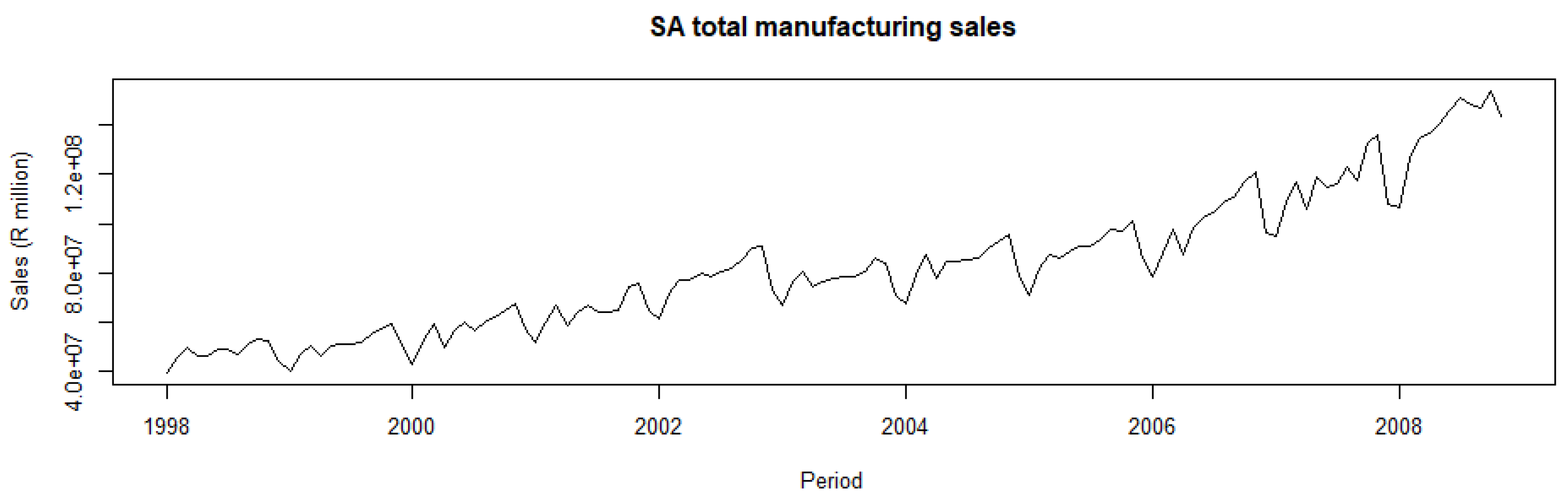
3.1. Data
3.2. ARIMA/SARIMA Model
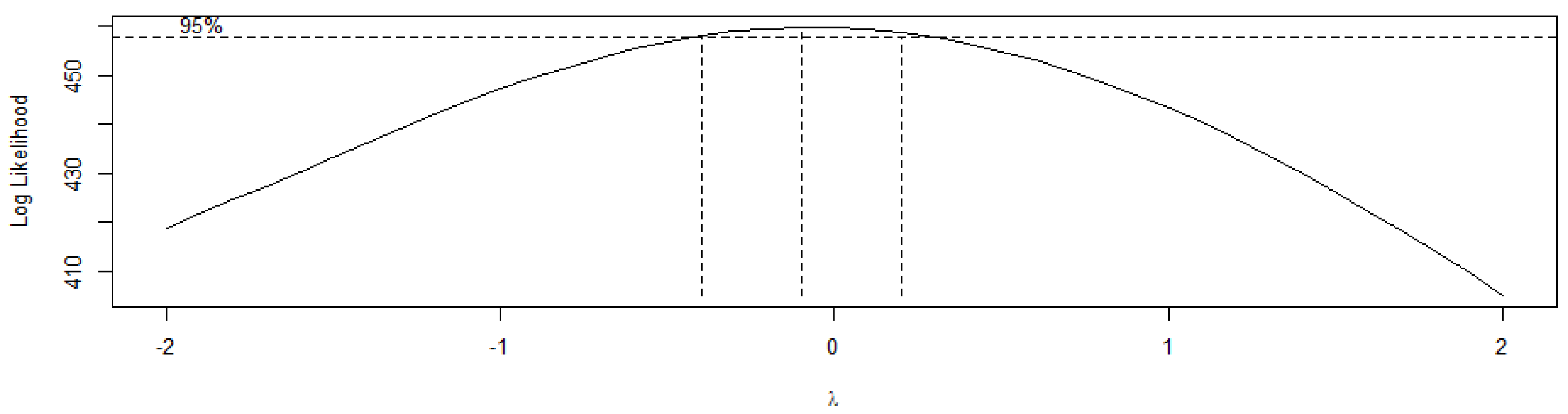
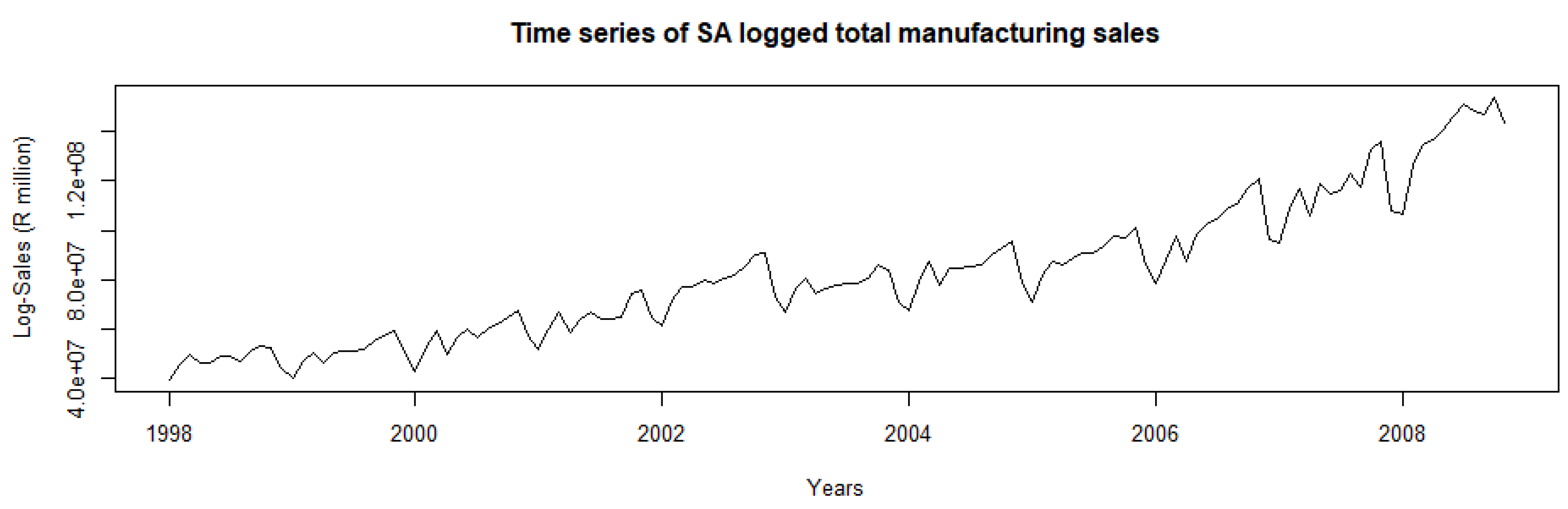
3.3. Data Transformation
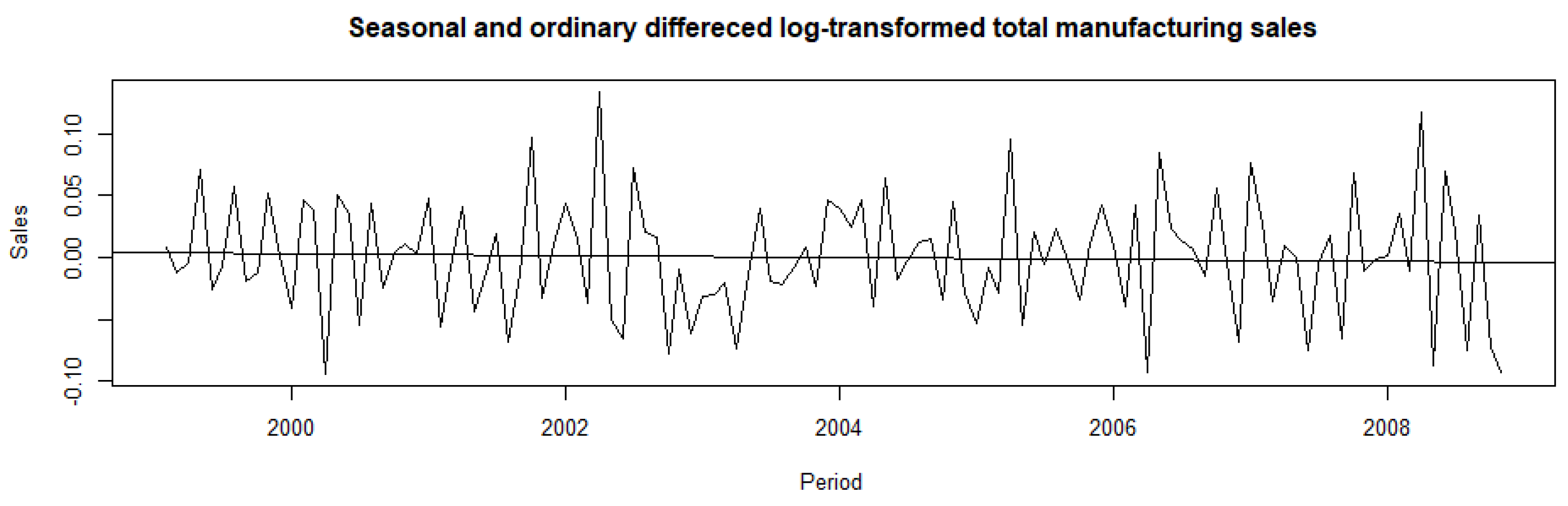
3.4. Argumented Dicky-Fuller (ADF) Test
3.5. Maximum Likelihood Estimator (MLE)
3.6. Model Selection and Accuracy Measures
4. Results
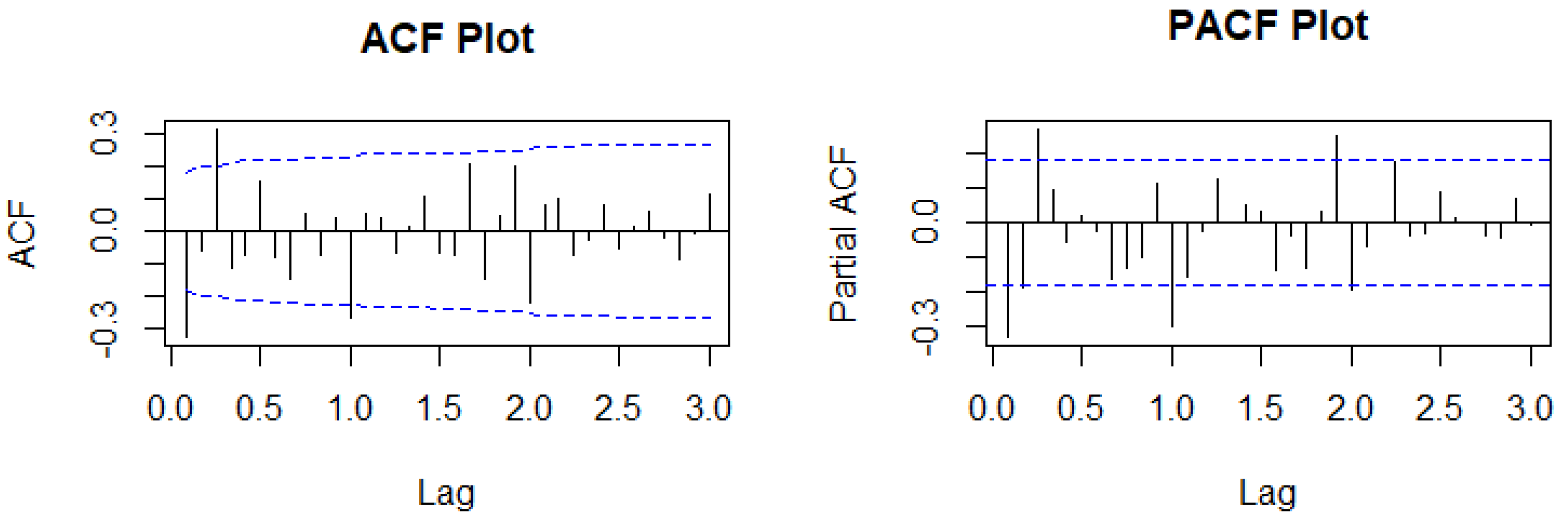
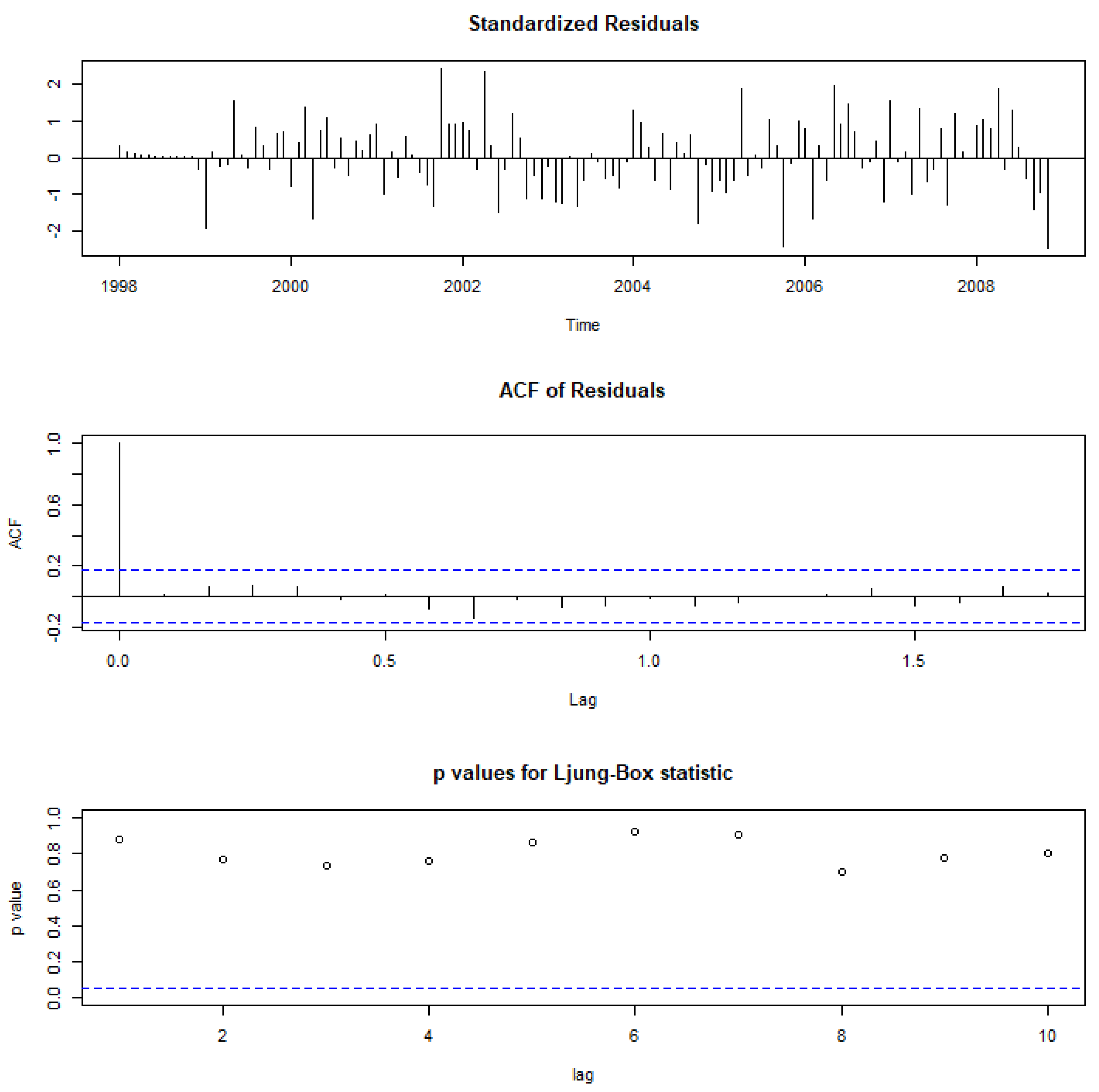
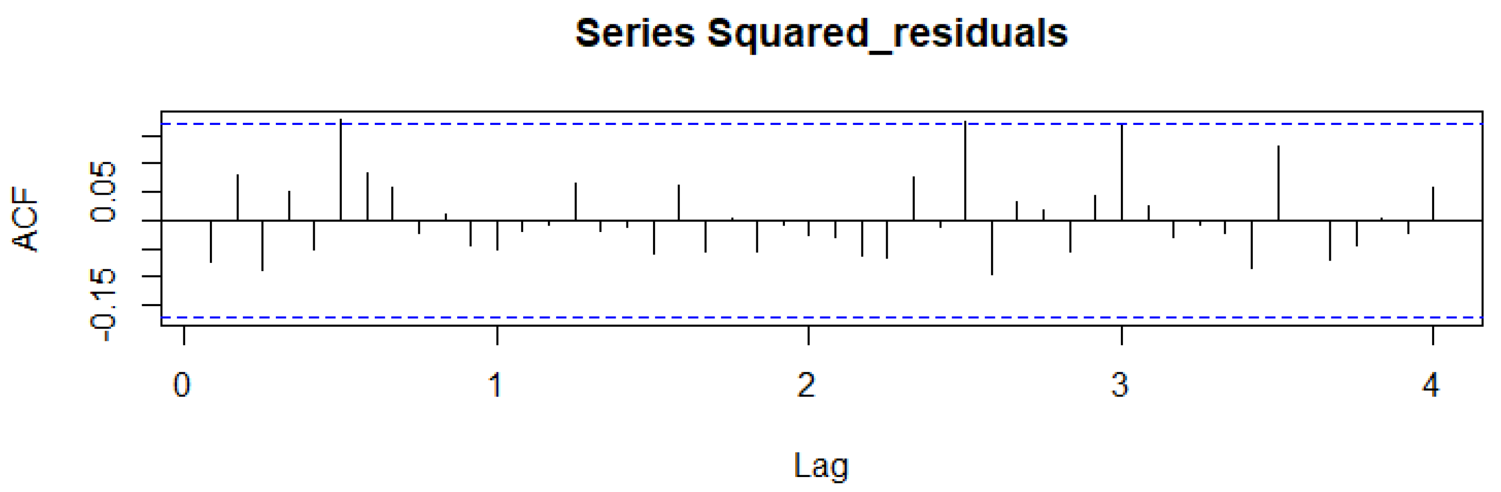
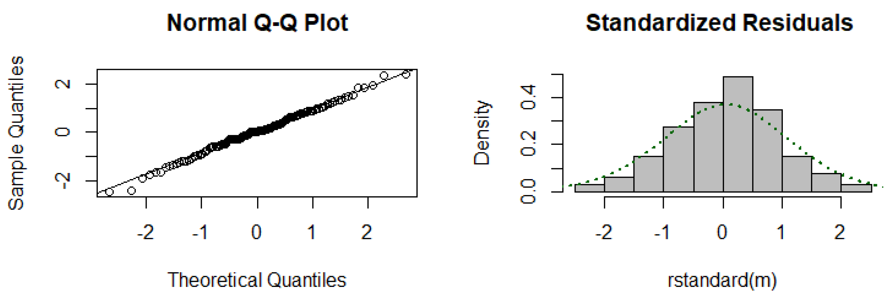
4.1. Descriptive Statistics and Model Identification Processes
4.2. In- and Out-of-Sample Forecasting
4.3. Discussion of Results
5. Conclusions
6. Recommendations
Author Contributions
Funding
Institutional Review Board Statement
Informed Consent Statement
Data Availability Statement
Conflicts of Interest
References
- Akhavan-Tabatabaei, Reza, Seyyed Mohammad Hossein Seyyedi, and Babak Shirazi. 2019. Application of SARIMA models in forecasting the monthly sales of a petrochemical company. Journal of the Chinese Chemical Society 66: 207–15. [Google Scholar]
- Bhorat, Haroon, and Christopher Rooney. 2017. State of Manufacturing in South Africa. University of Cape Town. Available online: http://www.dpru.uct.ac.za/sites/default/files/image_tool/images/36/Publications/Working_Papers/DPRU%20WP201702.pdf (accessed on 30 March 2023).
- Box, George Edward Pelham, and David Roxbee Cox. 1964. An analysis of transformations. Journal of the Royal Statistical Society: Series B 26: 211–52. [Google Scholar] [CrossRef]
- Box, George Edward Pelham, and Gwilym Jenkins. 1970. Time Series Analysis: Forecasting and Control. San Francisco: Holden-Day. [Google Scholar]
- Burke, Christopher, Sanusha Naidu, and Arno Nepgen. 2008. Scoping Study on China’s Relations with South Africa. Centre for Chinese Studies. University of Stellenbosch. Available online: https://www.econstor.eu/bitstream/10419/93164/1/58755861X.pdf (accessed on 25 March 2023).
- Dassanayake, Dilini Madushika Gamage Tennekoon, Ashani Nugaliyadde, and Yasitha Mallwaraachchi. 2011. Increasing Sales Productivity through Sales Forecasting Using ARIMA Models. Berlin/Heidelberg: Springer, pp. 1–11. [Google Scholar]
- Dellino, Gabriella, Meloni Carlo, and Roberto Revetria. 2015. Forecasting fresh food retail sales through time series models: A case study. Journal of Food Products Marketing 21: 530–52. [Google Scholar]
- Deloitte. 2019. Enhancing Manufacturing Competitiveness in South Africa. Available online: https://www2.deloitte.com/content/dam/Deloitte/dk/Documents/manufacturing/manufacturing-competitiveness-South-africa.pdf (accessed on 30 March 2023).
- Deloitte Manufacturing Competitiveness Report. 2013. Manufacturing for Growth Strategies for Driving Growth and Employment. Available online: https://www2.deloitte.com/content/dam/Deloitte/global/Documents/Manufacturing/gx_Mfg_Manufacturing_Growth_Volume01_05022013.pdf (accessed on 30 March 2023).
- Department of Energy (DoE). 2013. Aggregate Energy Balances. Available online: http://www.energy.gov.za/files/media/Energy_Balances.html (accessed on 17 February 2023).
- Dickey, David A., and Wayne A. Fuller. 1979. Distribution of the Estimates for Autoregressive Time Series with a Unit Root. Journal of the American Statistical Association 74: 427–31. [Google Scholar] [CrossRef]
- Edwards, Lawrence, and Rhys Jenkins. 2014. The Competitive Effects of China on the South African Manufacturing Sector. Southern African Labour and Development Research Unit (SALDRU), University of Cape Town. Available online: http://www.dpru.uct.ac.za/sites/default/files/image_tool/images/36/Publications/Policy_Briefs/DPRU%20PB%2014-40.pdf (accessed on 1 March 2023).
- Elder, John, and Apostolos Serletis. 2010. Oil price uncertainty. Journal of Money, Credit, and Banking 42: 1137–59. [Google Scholar] [CrossRef]
- European Commission (EC). 2012. A Stronger European Industry for Growth and Economic Recovery, COM (2012) 582 Final. Available online: https://www.eesc.europa.eu/en/our-work/opinions-information-reports/opinions/stronger-european-industry-growth-and-economic-recovery-industrial-policy-communication-update-com2012-582-final (accessed on 1 March 2023).
- Hyndman, Robin John, and George Athanasopoulos. 2018. Forecasting: Principles and Practice, 2nd ed. Melbourne: OTexts. Available online: https://otexts.com/fpp2/box-jenkins.html (accessed on 19 March 2023).
- Hyndman, Rob J., and Yeasmin Khandakar. 2008. Automatic time series forecasting: The forecast package for R. Journal of Statistical Software 26: 1–22. [Google Scholar]
- Industrial Development Corporation (IDC). 2013. Sustaining Employment Growth: The Role of Manufacturing and Structural Change. Available online: https://www.unido.org/sites/default/files/2013-12/UNIDO_IDR_2013_main_report_0.pdf (accessed on 1 March 2023).
- International Labour Office (ILO). 2011. The Global Crisis: Causes, Responses and Challenges. Available online: https://www.ilo.org/wcmsp5/groups/public/---dgreports/---dcomm/---publ/documents/publication/wcms_155824.pdf (accessed on 4 May 2023).
- Kapoor, Subhash. 2012. The 2007–2009 Financial Crisis: Causes, Impacts and the Need for New Regulations. Journal of Business and Economics 3: 340–47. [Google Scholar]
- Karimian, Seyedehsan, and Hamed Siavashi. 2021. Predicting Retail Sales Using LSTM and ARIMA Models. Journal of Retailing and Consumer Services 61: 102537. [Google Scholar]
- McKinsey Global Institute. 2012. Manufacturing the Future: The Next Era of Global Growth and Innovation. McKinsey Global Institute Report. Available online: https://time.com/wp-content/uploads/2015/03/manufacturing-the-future.pdf (accessed on 5 March 2023).
- Mnguni, Palesa, and Witness Simbanegavi. 2020. South African Manufacturing: A Situational Analysis. Available online: https://www.resbank.co.za/content/dam/sarb/publications/occasional-bulletin-of-economic-notes/2020/10410/OBEN%202002%20(South%20African%20Manufacturing%20A%20situational%20analysis)%20-%20November%202020.pdf (accessed on 5 March 2023).
- Mohamed, Seeraj. 2009. Impact of the Global Economic Crisis on the South African Economy. A Paper for the Africa Task Force Workshop 9–10 July, Pretoria. 2009. Available online: https://policydialogue.org/files/events/Mohamed_impact_of_global_financial_crisis.pdf (accessed on 4 May 2023).
- Moore, Tomoe, and Ali Mirzaei. 2014. The Impact of the Global Financial Crisis on Industry Growth. The Manchester School 84: 159–80. [Google Scholar] [CrossRef]
- Morris, Mike, and Gill Einhorn. 2008. Globalisation, Welfare and Competitiveness: The Impacts of Chinese Imports on the South African Clothing and Textile Industry. Competition and Change 12: 355–76. [Google Scholar] [CrossRef]
- Naudé, Wim, and Adam Szirmai. 2012. The Importance of Manufacturing in Economic Development: Past, Present and Future Perspectives. UNU-MERIT Working Papers 2012-041. pp. 1–67. Available online: http://collections.unu.edu/eserv/UNU:157/wp2012-041.pdf (accessed on 20 May 2023).
- Nisar, Waqar, Shaikh Farah, and Abdul Haseeb Khoja. 2020. Forecasting textile exports of Pakistan using ARIMA, ARIMAX and SARIMA models. Journal of Quantitative Economics 18: 403–18. [Google Scholar]
- Pao, Jenny Jie-Jen, and Danielle Simone Sullivan. 2017. Time Series Sales Forecasting. Available online: https://cs229.stanford.edu/proj2017/final-reports/5244336.pdf (accessed on 6 March 2023).
- Permatasari, Dwi, Endah Dwi Mustika, and Dwi Irianto. 2018. Short-term forecasting of daily newspaper sales using ARIMA models. Journal of Physics: Conference Series 997: 012075. [Google Scholar]
- Ratko, Zinaida, and Kaan Ulgen. 2009. The Impact of Economic Crisis on Small and Medium Enterprises: In Perspective of Swedish SMEs. Available online: https://www.diva-portal.org/smash/get/diva2:222654/FULLTEXT01.pdf (accessed on 4 May 2023).
- Rena, Ravinder, and Malindi Msoni. 2014. Global Financial Crises and its Impact on the South African Economy: A Further Update. Journal of Economics 5: 17–25. [Google Scholar] [CrossRef]
- Rizkya, Ira, Syahputri Khairani, Sari Rina Mustika, Siregar Irsal, and Utaminingrum Julianti. 2019. Autoregressive Integrated Moving Average (ARIMA) Model of Forecast Demand in Distribution Centre. In IOP Conference Series: Materials Science and Engineering. Bristol: IOP Publishing, vol. 598, p. 012071. [Google Scholar] [CrossRef]
- Sharma, Hermant, and Sukhdeo Singh Burark. 2015. Forecasting Price of Sorghum in Ajmer Market of Rajasthan: An Empirical Study. Annals of Agricultural Research New Series 36: 212–18. [Google Scholar]
- Shukla, Manish, and Sanjay Jharkharia. 2013. Applicability of ARIMA Models in Wholesale Vegetable Market: An Investigation. International Journal of Information Systems and Supply Chain Management 6: 105–19. [Google Scholar] [CrossRef]
- South African Government. 2023. South Africa’s Grey Listing is an Opportunity to Strengthen the Fight against Financial Crimes. Available online: https://www.gov.za/blog/south-africa%E2%80%99s-grey-listing-opportunity-strengthen-fight-against-financial-crimes (accessed on 30 March 2023).
- Statistics South Africa. 2016. Quarterly Labour Force Survey, Quarter 1: 2016. Pretoria: Statistics South Africa. [Google Scholar]
- Steytler, Nico, and Derek Powell. 2010. The Impact of the Global Financial Crisis on Decentralized Government in South Africa. Available online: https://www.cairn.info/revue-l-europe-en-formation-2010-4-page-149.htm#no23 (accessed on 4 May 2023).
- Venter, Johann Christoffel. 2009. Business Cycles in South Africa during the Period 1999 to 2007, Quarterly Bulletin 253. Pretoria: South African Reserve Bank, pp. 61–69. [Google Scholar]
- Verick, Sher. 2010. The Global Financial Crisis and South Africa: What Has Been the Impact on the Labour Market? Geneva: International Labour Office. Available online: https://www.wiego.org/sites/default/files/migrated/publications/files/Verick_The_global_financial_crisis_and_south_africa_Sher_Verick.pdf (accessed on 4 May 2023).
- Wanjuki, Teddy Mutugi, Adolphus Wagala, and Dennis Karuri Muriithi. 2021. Forecasting Commodity Price Index of Food and Beverages in Kenya Using Seasonal Autoregressive Integrated Moving Average (SARIMA) Models. EJ-MATH, European Journal of Mathematics and Statistics 2: 50–63. [Google Scholar] [CrossRef]
- World Bank. 2018. South Africa Economic Update: Jobs and Inequality, Edition 11. Available online: http://pubdocs.worldbank.org/en/798731523331698204 (accessed on 4 May 2023).
- World Bank. 2020. South Africa Economic Update, October 2020: From Crisis to Renewal: Toward a More Inclusive and Sustainable Economic Future. Washington, DC: World Bank. [Google Scholar]


| Minimum | Maximum | Mean | Std. Deviation | Skewness | Kurtosis |
|---|---|---|---|---|---|
| 39,275,290 | 153,975,510 | 82,029,512 | 27,892,621 | 0.7 | −0.19 |
| Dickey–Fuller | Lag Order | p-Value |
|---|---|---|
| −3.1304 | 5 | 0.1065 |
| Dickey–Fuller | Lag Order | p-Value |
|---|---|---|
| −3.8468 | 4 | 0.01911 |

| Model | AIC | BIC | RMSE |
|---|---|---|---|
| SARIMA (2,1,1)(2,1,1)12 model without drift | −447.83 | −428.44 | 0.0311 |
| SARIMA (2,1,2)(2,1,1)12 model without drift | −456.86 | −434.7 | 0.0297 |
| SARIMA (2,1,0)(2,1,1)12 model without drift | −442.9 | −426.28 | 0.0320 |
| SARIMA (1,1,1)(2,1,1)12 model without drift | −438.19 | −421.57 | 0.0327 |
| SARIMA (0,1,1)(2,1,1)12 model without drift | −438.82 | −424.97 | 0.0328 |
| SARIMA (1,1,2)(1,0,0)12 model with drift | −426.61 | −409.41 | 0.0412 |
| SARIMA (2,1,2)(2,0,0)12 model with drift | −446.91 | −423.97 | 0.0369 |
| Parameter | Coefficient/ Parameter Estimate | Standard Error (SE) | Test Statistic | p-Value |
|---|---|---|---|---|
| −0.9425 | 0.1082 | −8.7117 | <0.0001 | |
| −0.8197 | 0.0861 | −9.5151 | <0.0009 | |
| −0.2534 | 0.1515 | −1.6730 | 0.0943 | |
| −0.2884 | 0.1276 | −2.2599 | 0.0238 | |
| 0.5579 | 0.1628 | 3.4266 | 0.0006 | |
| 0.5015 | 0.1096 | 4.5771 | <0.0001 | |
| −0.6343 | 0.1513 | −4.1917 | <0.0001 |
Disclaimer/Publisher’s Note: The statements, opinions and data contained in all publications are solely those of the individual author(s) and contributor(s) and not of MDPI and/or the editor(s). MDPI and/or the editor(s) disclaim responsibility for any injury to people or property resulting from any ideas, methods, instructions or products referred to in the content. |
© 2023 by the authors. Licensee MDPI, Basel, Switzerland. This article is an open access article distributed under the terms and conditions of the Creative Commons Attribution (CC BY) license (https://creativecommons.org/licenses/by/4.0/).
Share and Cite
Makoni, T.; Chikobvu, D. Assessing and Forecasting the Long-Term Impact of the Global Financial Crisis on Manufacturing Sales in South Africa. Economies 2023, 11, 158. https://doi.org/10.3390/economies11060158
Makoni T, Chikobvu D. Assessing and Forecasting the Long-Term Impact of the Global Financial Crisis on Manufacturing Sales in South Africa. Economies. 2023; 11(6):158. https://doi.org/10.3390/economies11060158
Chicago/Turabian StyleMakoni, Tendai, and Delson Chikobvu. 2023. "Assessing and Forecasting the Long-Term Impact of the Global Financial Crisis on Manufacturing Sales in South Africa" Economies 11, no. 6: 158. https://doi.org/10.3390/economies11060158